Tight contact structures on the Brieskorn spheres $-\Sigma(2,3,6n-1)$ and contact invariants

Abstract.

We compute the Ozsváth–Szabó contact invariants for all tight contact structures on the manifolds $-\Sigma(2,3,6n-1)$ using twisted coefficient and a previous computation by the first author and Ko Honda. This computation completes the classification of the tight contact structures in this family of $3$-manifolds.

1. Introduction

The family of $3$-manifolds $-\Sigma(2,3,6n-1)$ defined by the surgery diagram in Figure 1 has been an exciting playground for contact topologists for many years, and any progress in the knowledge of the tight contact structures in this family has led us to progress in our understanding of three-dimensional contact topology.

These manifolds first were used by Lisca and Matić in [17] to give an example of the power of the recently discovered Seiberg–Witten invariants in distinguishing tight contact structures. Later Etnyre and Honda [2] proved that $-\Sigma(2,3,5)$ supports no tight contact structure, giving the first example of such a manifold. Tight contact structures on $-\Sigma(2,3,17)$ were instrumental in the first vanishing theorem for the Ozsváth–Szabó contact invariant in [5]. Finally the first author proved in [3] that $-\Sigma(2,3,6n-1)$ carries a strongly fillable contact structure which is not Stein fillable when $n\geq 3$, thus showing that strong and Stein fillability are different concepts in dimension three.

The goal of this paper is to give a complete classification of tight contact structures on manifolds in this family, and to do that we will compute their Ozsváth–Szabó contact invariants. The proof is a delicate computation using Heegaard Floer homology with twisted coefficients.

\psfrag{0}{$0$}\psfrag{a}{$-n$}\includegraphics[width=113.81102pt]{nodo}

Figure 1. Surgery diagram for $-\Sigma(2,3,6n-1)$

It has been known for a while that $-\Sigma(2,3,6n-1)$ supports at most $\frac{n(n-1)}{2}$ distinct contact structures up to isotopy. We will denote them by $\eta_{i,j}^{n}$ where $0\leq i\leq n-2$ and $-n+i+2\leq j\leq n-i-2$ with $j\equiv n-i$ (mod $2$). The geometric meaning of the indices $i$ and $j$ will be explained in the next section. In order to simplify the exposition we define the following notation for the sets of indices of the contact structures $\eta_{i,j}^{n}$:

Definition 1.1.

For any $n\geq 2$ we define

$${\mathcal{P}}_{n}=\left\{(i,j)\in\mathbb{Z}\times\mathbb{Z}:\begin{array}[]{l}0\leq i\leq n-2,\\ |j|\leq n-i-2\text{ with }j\equiv n-i\;({\rm mod}\,2)\end{array}\right\}.$$

We can visualize ${\mathcal{P}}_{n}$ (and the contact structures indexed by its elements) as a triangle with $n-1$ rows and $(n-2,0)$ at its upper vertex. For example for $n=5$ we have:

(1) $$\begin{matrix}&&&\eta_{3,0\phantom{-}}^{5}&&&\\ &&\eta_{2,-1}^{5}&&\eta_{2,1\phantom{-}}^{5}&&\\ &\eta_{1,-2}^{5}&&\eta_{1,0\phantom{-}}^{5}&&\eta_{1,2\phantom{-}}^{5}&\\ \eta_{0,-3}^{5}&&\eta_{0,-1}^{5}&&\eta_{0,1\phantom{-}}^{5}&&\eta_{0,3\phantom{-}}^{5}\\ \end{matrix}$$

For any $n$, the contact structures on the bottom row (i.e. those with $i=0$) are obtained by Legendrian surgery on all possible Legendrian realizations of the link in Figure 1 (see Figure 9), and therefore are Stein fillable. All other contact structures are strongly symplectically fillable, and the top one (i.e. $\eta_{n-2.0}^{n}$) is known not to be Stein fillable by [3]. No Stein filling is known for $\eta^{n}_{i,j}$ when $i>0$. Therefore we conjecture the following:

Conjecture 1.2.

The contact structures $\eta_{i,j}^{n}$ are not Stein fillable if $i>0$.

Now we can state the main result of this article:

Theorem 1.3.

Let $c(\eta^{n}_{i,j})$ denote the Ozsváth–Szabó contact invariant of $\eta^{n}_{i,j}$. We can choose representatives for $c(\eta^{n}_{0,j})$ such that, for any $(i,j)\in{\mathcal{P}}_{n}$, the contact invariant of $\eta_{i,j}^{n}$ is computed by the formula:

(2) $$c(\eta_{i,j}^{n})=\sum\limits_{k=0}^{i}(-1)^{k}\binom{i}{k}c(\eta_{0,j-i+2k}^{n}).$$

We can reformulate Theorem 1.3 in plain English as follows. Any $(i,j)\in{\mathcal{P}}_{n}$ determines a sub-triangle ${\mathcal{P}}_{n}(i,j)\subset{\mathcal{P}}_{n}$ with top vertex at $(i,j)$ defined as

$${\mathcal{P}}_{n}(i,j)=\left\{(k,l)\in{\mathcal{P}}_{n}:0\leq k\leq i\quad\text{and}\quad j-k\leq l\leq j+k\right\}.$$

The contact invariant of $\eta_{i,j}^{n}$ is then a linear combination of the invariants of the contact structures parametrized by the pairs in the base of ${\mathcal{P}}_{n}(i,j)$. In order to compute the coefficients we associate natural numbers to the elements of ${\mathcal{P}}_{n}(i,j)$, starting by associating $1$ to the vertex $(i,j)$, and going downward following the rule of the Pascal triangle. Then the numbers associated to the elements in the bottom row, taken with alternating signs, are the coefficients of the contact invariants of the corresponding contact structures in the sum in Equation (2).

Olga Plamenevskaya proved in [25] that the contact invariants of the contact structures parametrized by the elements in the bottom row of ${\mathcal{P}}_{n}$ (i.e. those with $i=0$) are linearly independent, so all $\eta_{i,j}^{n}$ have distinct contact invariants. Thus we have the following corollary:

Corollary 1.4.

$-\Sigma(2,3,6n-1)$ admits exactly $\frac{n(n-1)}{2}$ distinct isotopy classes of tight contact structures with nonzero and pairwise distinct Ozsváth–Szabó contact invariants.

The same classification result could probably be derived also from Wu’s work on Legendrian surgeries [27] and from the computation of the contact invariants with twisted coefficients of contact manifolds with positive Giroux’s torsion in [6]. However it is not clear how to obtain a complete description of the contact invariants as in Theorem 1.3 from that approach.

Acknowledgement

This work was started when the authors met at the 2008 France-Canada meeting; we therefore thank the Canadian Mathematical Society, the Société Mathématique de France and CIRGET for their hospitality. We also thank Ko Honda for suggesting the problem to the first author and helping him to work out the upper bound in 2001, and Thomas Mark for useful explanations about Heegaard Floer homology with twisted coefficients. We finally thank the anonymous referees for helping us improve the exposition. The first author acknowledges partial support from the ANR project ‘Floer Power.’

2. Contact structures on $-\Sigma(2,3,6n-1)$

2.1. Construction of the tight contact structures

We introduce the notation

$$Y_{n}=-\Sigma(2,3,6n-1)$$

and, coherently with the standard surgery convention, we define $Y_{\infty}$ to be the $3$-manifold obtained by $0$-surgery on the right-handed trefoil knot. We describe $Y_{\infty}$ as a quotient of $T^{2}\times\mathbb{R}$ (with coordinates $(x,y)$ on $T^{2}$ and $t$ on $\mathbb{R}$):

$$Y_{\infty}=T^{2}\times\mathbb{R}/(\mathbf{v},t)=(A\mathbf{v},t-1)$$

where $A\colon T^{2}\to T^{2}$ is induced by the matrix $\left(\begin{matrix}1&1\\ -1&0\end{matrix}\right)$. In [9] Giroux constructed a family of weakly symplectically fillable contact structures $\xi_{i}$ on $Y_{\infty}$ for $i\geq 0$ as follows. For any $i\geq 0$, fix a function $\varphi_{i}\colon\mathbb{R}\to\mathbb{R}$ such that:

• $\varphi_{i}^{\prime}(t)>0$ for any $t\in\mathbb{R}$, and

• $(2i+1)\pi\leq\sup\limits_{t\in\mathbb{R}}(\varphi_{i}(t+1)-\varphi_{i}(t))<2(i+1)\pi$.

By condition $(1)$ the $1$-form

$$\alpha_{i}=\sin(\varphi_{i}(t))dx+\cos(\varphi_{i}(t))dy$$

defines a contact structure $\tilde{\xi}_{i}=\ker\alpha_{i}$ on $T^{2}\times\mathbb{R}$. Moreover it is possible to choose $\varphi_{i}$ such that the contact structure $\tilde{\xi}_{i}$ (but not the $1$-form $\alpha_{i}$ in general) is invariant under the action $({\mathbf{v}},t)\mapsto(A{\mathbf{v}},t-1)$ and therefore defines a contact structure $\xi_{i}$ on $Y_{\infty}$.

Proposition 2.1 ([9, Proposition 2]).

For any fixed integer $i\geq 0$ the contact structure $\xi_{i}$ is tight, and its isotopy class does not depend on the chosen function $\varphi_{i}$.

The knot

$$F=\{\mathbf{0}\}\times\mathbb{R}/(\mathbf{0},t)=(\mathbf{0},t-1)\subset Y_{\infty}$$

is Legendrian with respect to $\xi_{i}$ for any $i$. Given a framing on $F$, we define the twisting number of $F$ with respect to $\xi_{i}$, denoted by $tn(F,\xi_{i})$, as the number of times $\xi_{i}|_{F}$ rotates with respect to the framing on $F$. The twisting number depends on the framing and is a generalization of the Thurston-Bennequin number to knots which are not necessarily null-homologous.

In [5] the first author proved the following properties of $F$:

Proposition 2.2 ([5, Lemma 3.5]).

There exists a framing on $F$ such that:

1. $tn(F,\xi_{i})=-i-1$

2. performing surgery on $Y_{\infty}$ along $F$ with surgery coefficient $-n$ yields $Y_{n}$.

If $Y_{\infty}$ is identified with the $0$-surgery on the right-handed trefoil knot, then $F$ corresponds to a meridian, i.e. it is the knot labeled by “$-n$” in Figure 1. The framing on $F$ from Proposition 2.2 then corresponds to the Seifert framing of the meridian in the surgery diagram shown in Figure 1.

Moreover, even though $F$ is nontrivial in homology, we can define a rotation number ${\tt rot}(\mathcal{L},\xi_{i})$ for an oriented Legendrian knot $\mathcal{L}\subset(Y_{\infty},\xi_{i})$ smoothly isotopic to $F$: we set ${\tt rot}(F,\xi_{i})=0$ for all $i$ and define ${\tt rot}(\mathcal{L},\xi_{i})={\tt rot}(\mathcal{L}\cup\overline{F},\xi_{i})$, where $\overline{F}$ denotes $F$ with the opposite orientation. We do not need to reference a Seifert surface for $\mathcal{L}\cup\overline{F}$ because $c_{1}(\xi_{i})=0$. We are finally in position to give a precise definition of the contact structures $\eta_{i,j}^{n}$ and, at the same time, to explain the topological meaning of the indices $i$ and $j$.

Definition 2.3.

For any $(i,j)\in{\mathcal{P}}_{n}$ the contact manifold $(Y_{n},\eta_{i,j}^{n})$ is obtained by Legendrian surgery on $(Y_{\infty},\xi_{i})$ along a Legendrian knot $F_{i,j}$ which is obtained by applying $n-i-2$ stabilizations to $F$, choosing their signs so that ${\tt rot}(F_{i,j},\xi_{i})=j$.

In order to complete the classification of tight contact structures on $Y_{n}$ we need two steps:

1. prove that there are at most $\frac{n(n-1)}{2}$ distinct tight contact structures on $Y_{n}$ up to isotopy, and

2. prove that the contact structures $\eta_{i,j}^{n}$ are all pairwise nonisotopic.

The first step is a folklore result which follows from the arguments of [8], but nevertheless we are going to sketch its proof in the next subsection. The second step is a corollary of Theorem 1.3, which will be proved in the last section.

2.2. Upper bound

The upper bound on the number of tight contact structures on $Y_{n}$ can be easily obtained following the strategy in [8], where the tight contact structures on $-\Sigma(2,3,11)$ have been classified. In fact, the manifold denoted by $Y_{n}$ in this paper corresponds to the manifold denoted by $M(-\frac{1}{2},\frac{1}{3},\frac{n}{6n-1})$ in [8]. We recall the conventions of that paper.

\psfrag{e0}{\small$0$}\psfrag{r1}{\small$2$}\psfrag{r2}{\small$-3$}\psfrag{r3}{\small$-\frac{6n-1}{n}$}\includegraphics[width=142.26378pt]{1}

Figure 2. Surgery diagram for $-\Sigma(2,3,6n-1)$

The manifold $Y_{n}$ can be described also by the surgery diagram shown in Figure 2. See [8, Figure 17] for a sequence of Kirby move from the diagram in Figure 2 to the diagram in Figure 1.

The surgery diagram 2 describes a splitting of $Y_{n}$ into four pieces:

$$Y_{n}=(\Sigma\times S^{1})\cup V_{1}\cup V_{2}\cup V_{3}$$

where $\Sigma$ is a three-punctured sphere, i.e. a pair of pants, and $V_{1}$, $V_{2}$, and $V_{3}$ are solid tori. We orient the boundary of $\Sigma\times S^{1}$ by the “inward normal vector first” convention (i.e. we give it the opposite of the usual boundary orientation), and identify each component $\partial(S^{1}\times\Sigma)_{i}$ of $\partial(S^{1}\times\Sigma)$ with $\mathbb{R}^{2}/\mathbb{Z}^{2}$ by setting $\binom{0}{1}$ as the direction of the $S^{1}$-fibers and $\binom{1}{0}$ as the direction of $\partial(\{pt\}\times\Sigma)$.

We also fix identifications of $\partial V_{i}$ with $\mathbb{R}^{2}/\mathbb{Z}^{2}$ by setting $\binom{1}{0}$ as the direction of the meridian. Then we obtain the manifold $Y_{n}$ by attaching the solid tori $V_{i}$ to $S^{1}\times\Sigma$, where the attaching maps $A_{i}\colon\partial V_{i}\to\partial(S^{1}\times\Sigma)_{i}$ are given by

$$A_{1}=\left(\begin{matrix}2&-1\\ 1&0\end{matrix}\right),\qquad A_{2}=\left(\begin{matrix}3&1\\ -1&0\end{matrix}\right),\qquad A_{3}=\left(\begin{matrix}6n-1&6\\ -n&-1\end{matrix}\right).$$

This construction induces a Seifert fibration on $Y_{n}$ where the curves $S^{1}\times\{pt\}$ are regular fibers, and the cores of the solid tori $V_{i}$ are the singular fibers. The regular fibers have a natural framing coming from the Seifert fibration, and the singular fibers have a framing coming from the chosen identification of $\partial V_{i}$ with $\mathbb{R}^{2}/\mathbb{Z}^{2}$. These framings can be extended in a unique way to all curves which are isotopic to fibers because the manifolds $Y_{n}$ are integer homology spheres. Therefore, for a contact structure $\xi$ on $Y_{n}$, we can speak about the twisting number $tn(L,\xi)$ of a Legendrian curve $L$ which is isotopic to a fiber of the Seifert fibration.

Definition 2.4.

For any contact structure $\xi$ on $Y_{n}$, we define the maximal twisting number of $\xi$ as

$$t(\xi)=\max_{L\in{\mathfrak{L}}}\min\{tn(L,\xi),0\}$$

where ${\mathfrak{L}}$ is the set of all Legendrian curves in $Y_{n}$ which are smoothly isotopic to a regular fiber.

The maximal twisting number is clearly an isotopy invariant of the contact structure $\xi$.

Proposition 2.5.

Let $\xi$ be a tight contact structure on $Y_{n}$. Then $t(\xi)<0$.

Proof.

The proof is the same as in [8, Theorem 4.14]. ∎

Lemma 2.6.

If $\xi$ can be isotoped so that the singular fiber $F_{2}$ is a Legendrian curve with twisting number $tb(F_{2},\xi)=-1$, then there is a Legendrian regular fiber with twisting number zero. In particular $\xi$ is overtwisted.

Proof.

We isotope $F_{1}$ so that it becomes a Legendrian curve with twisting number $tb(F_{1})=k_{1}\ll 0$. Let $V_{1}$ and $V_{2}$ be standard neighborhoods of $F_{1}$ and $F_{2}$ respectively. We assume that $\partial(Y_{n}\setminus V_{1})$ and $\partial(Y_{n}\setminus V_{2})$ have Legendrian rulings of infinite slope, and take a convex annulus $A$ with boundary on a Legendrian ruling curve of $\partial(Y_{n}\setminus V_{1})$ and one of $\partial(Y_{n}\setminus V_{2})$.

The slope of $\partial(Y_{n}\setminus V_{1})$ is $\frac{k_{1}}{2k_{1}-1}$, and the slope of $\partial(Y_{n}\setminus V_{2})$ is $-\frac{1}{2}$. As long as $k_{1}\leq-1$ the Imbalance Principle [13, Proposition 3.17] provides a bypass along a Legendrian ruling curve of $\partial(Y_{n}\setminus V_{1})$. Therefore we can apply the Twisting Number Lemma [13, Lemma 4.4] to increase the twisting number $k_{1}$ of a singular fiber by one up to $k_{1}=0$, which corresponds to slope $0$ on $\partial(Y_{n}\setminus V_{1})$. At this point there are two possibilities for the annulus $A$ between $\partial(Y_{n}\setminus V_{1})$ and $\partial(Y_{n}\setminus V_{2})$: either $A$ carries a bypass for $\partial(Y_{n}\setminus V_{1})$, or it does not. If such a bypass exists, then the slope of $\partial(Y_{n}\setminus V_{1})$ can be made infinite, and we are done. If there is no such a bypass, cutting along $A$ and rounding the edges yields a torus with slope $0$ (see [13, Lemma 3.11]), which is $-n$ when measured in $\partial V_{3}$. In this case by [13, Proposition 4.16] we find a convex torus in $V_{3}$ with slope $-n+\frac{1}{6}$ , which corresponds to infinite slope in $\partial(M\setminus V_{3})$. ∎

Proposition 2.7.

Let $\xi$ be a tight contact structure on $Y_{n}$. Then $t(\xi)=-6k+1$ for some $k$ with $0<k<n-1$.

Proof.

Let $t(\xi)=-q$. We start by assuming that the contact structure has been isotoped so that there is a Legendrian regular fiber $L$ with twisting number $tb(L,\xi)=-q$, and the singular fibers $F_{i}$ are Legendrian curves with twisting numbers $k_{i}\ll 0$. We take $V_{i}$ to be a standard neighborhood of the singular fiber $F_{i}$ disjoint from $L$ for $i=1,2,3$.

The slopes of $\partial V_{i}$ are $\frac{1}{k_{i}}$, while the slopes of $\partial(Y_{n}\setminus V_{i})$ are $\frac{k_{1}}{2k_{1}-1}$, $-\frac{k_{2}}{3k_{2}+1}$, and $-\frac{nk_{3}+1}{(6n-1)k_{3}+6}$ respectively. We also assume that the Legendrian ruling on each $\partial(Y_{n}\setminus V_{i})$ has infinite slope, and take convex annuli $A_{i}$ whose boundary consists of $L$ and of a Legendrian ruling curve of $\partial(Y_{n}\setminus V_{i})$ for $i=1,2$. If $2k_{1}-1<-q$ the Imbalance Principle [13, Proposition 3.17] provides a bypass along a Legendrian ruling curve either in $\partial(Y_{n}\setminus V_{1})$ or in $\partial(Y_{n}\setminus V_{2})$. Then we can apply the Twisting Number Lemma [13, Lemma 4.4] to increase the twisting number $k_{i}$ of a singular fiber by one until either $2k_{1}-1<-q$, or $k_{1}=0$. Similarly we use the annulus $A_{2}$ to increase $k_{2}$ until either $3k_{2}+1=-q$, or $k_{2}=-1$.

If $2k_{1}-1=3k_{2}+1=-q$ we can write $k_{1}=-3k+1$, $k_{2}=-2k$, and $q=6k-1$ for some $k>0$. Take a convex annulus $A$ with Legendrian boundary consisting of a Legendrian ruling curve of $\partial(Y_{n}\setminus V_{1})$ and of one of $\partial(Y_{n}\setminus V_{2})$. The dividing set of $A$ contains no boundary parallel arc; otherwise we could attach a bypass to either $\partial(Y_{n}\setminus V_{1})$ or to $\partial(Y_{n}\setminus V_{2})$, and the vertical Legendrian ruling curves of the resulting torus would contradict the maximality of $-q$. If we cut $Y_{n}\setminus(V_{1}\cup V_{2})$ along $A$ and round the edges, we obtain a torus with slope $-\frac{k}{6k+1}$ isotopic to $\partial(Y_{n}\setminus V_{3})$. Its slope corresponds to $-n+k$ on $\partial V_{3}$. If $k\geq n$ we can find a standard neighborhood $V_{3}^{\prime}$ of $F_{3}$ with infinite boundary slope by [13, Proposition 4.16]. This boundary slope becomes $-\frac{1}{6}$ if measured with respect to $\partial(Y_{n}\setminus V_{3}^{\prime})$, contradicting $q>6n-1$. (Remember that we are assuming $n\geq 2$.) ∎

Proposition 2.8.

There are at most $\frac{n(n-1)}{2}$ isotopy classes of tight contact structures on $Y_{n}$.

Proof.

If $t(\xi)=-6k+1$ we can find a neighborhood $V_{3}$ of $F_{3}$ such that $\partial(Y_{n}\setminus V_{3})$ has slope $-\frac{k}{6k+1}$. This slope corresponds to $-n+k$ on $\partial V_{3}$. By the classification of tight contact structures on solid tori [13, Theorem 2.3], there are $n-k$ tight contact structures on $V_{3}$. Since $k$ ranges from $1$ to $n-1$, we have a total count of at most $\frac{n(n-1)}{2}$ tight contact structures on $Y_{n}$. ∎

3. Heegaard Floer homology with twisted coefficients

In the computation of the contact invariants of $\eta_{i,j}$ we will use the Heegaard Floer homology groups with twisted coefficients. Since this theory is not as well known as the usual Heegaard Floer theory, we give a brief review of its properties. A more detailed exposition for the interested reader can be found in the original papers [22, 24] and in [15].

Let $Y$ be a closed, connected and oriented $3$-manifold. In the following, singular cohomology groups will always be taken with integer coefficients, unless a different abelian group is explicitly indicated. Given a module $M$ over the group algebra $\mathbb{Z}[H^{1}(Y)]$ and a ${\rm Spin}^{c}$-structure $\mathfrak{t}\in{\rm Spin}^{c}(Y)$, in [22, Section 8] Ozsváth and Szabó defined the Heegaard Floer homology group with twisted coefficients $\underline{\widehat{HF}}(Y,\mathfrak{t};M)$, which has a natural structure of a $\mathbb{Z}[H^{1}(Y)]$-module. When we omit the ${\rm Spin}^{c}$-structure from the notation, we understand that we take the direct sum over all ${\rm Spin}^{c}$-structures of $Y$. Defining $\underline{\widehat{HF}}(Y,\mathfrak{t};M)$ as a $\mathbb{Z}[H_{2}(Y)]$-module would be a somewhat more natural choice and would lead to simpler formulas; however we have chosen to follow the exposition in the original papers.

Two modules $M$ are of particular interest: the free module of rank one $M=\mathbb{Z}[H^{1}(Y)]$, and the module $M=\mathbb{Z}$ with the trivial action of $H^{1}(Y)$. In the first case we will denote $\underline{\widehat{HF}}(Y;M)=\underline{\widehat{HF}}(Y)$, and in the second case $\underline{\widehat{HF}}(Y;M)=\widehat{HF}(Y)$. The automorphism $x\mapsto-x$ of $H^{1}(Y)$ induces an involution of $\mathbb{Z}[H^{1}(Y)]$ which we call conjugation and denote by $r\mapsto\bar{r}$. If $M$ is a module over $\mathbb{Z}[H^{1}(Y)]$, we define a new module $\overline{M}$ by taking $M$ as an additive group, and equipping it with the multiplication $r\otimes m\mapsto\bar{r}\cdot m$.

To a cobordism $W$ from $Y_{0}$ to $Y_{1}$, in [24] Ozsváth and Szabó associated morphisms between the Heegaard Floer homology groups with twisted coefficients. However there is an extra complication which is absent in the untwisted case: the groups are usually modules over different rings, and we need to define a “canonical” way to transport coefficients across a cobordism. Let us define

$$K(W)=\ker\left(H^{2}(W,\partial W)\to H^{2}(W)\right).$$

Its group algebra $\mathbb{Z}[K(W)]$ has the structure of both a $\mathbb{Z}[H^{1}(Y_{0})]$-module and a $\mathbb{Z}[H^{1}(Y_{1})]$-module induced by the connecting homomorphism $\delta\colon H^{1}(\partial W)\to H^{2}(W,\partial W)$ for the relative long exact sequence of the pair $(W,\partial W)$. Therefore we can define the $\mathbb{Z}[H^{1}(Y_{1})]$-module $M(W)$ as

$$M(W)=\overline{M}\otimes_{\mathbb{Z}[H^{1}(Y_{0})]}\mathbb{Z}[K(W)].$$

Theorem 3.1 ([24, Theorem 3.8]).

Any cobordism $W$ from $Y_{0}$ to $Y_{1}$ with a ${\rm Spin}^{c}$-structure $\mathfrak{s}\in{\rm Spin}^{c}(W)$ induces an anti-$\mathbb{Z}[H^{1}(Y_{0})]$-linear map

$$F_{W,\mathfrak{s}}\colon\underline{\widehat{HF}}(Y_{0},\mathfrak{s}|_{Y_{0}};M)\to\underline{\widehat{HF}}(Y_{1},\mathfrak{s}|_{Y_{1}};M(W))$$

which is well defined up to sign, right multiplication by invertible elements of $\mathbb{Z}[H^{1}(Y_{1})]$, and left multiplication by invertible elements of $\mathbb{Z}[H^{1}(Y_{0})]$.

We will denote the equivalence class of such a map by $[F_{W,\mathfrak{s}}]$. The anti-linearity of the cobordism maps is a consequence of the unnatural choice of coefficients. The reason for it is that $W$ induces the opposite orientation on $Y_{0}$ and hence a negative sign appears in comparing the Poincaré duality on $W$ and $Y_{0}$.

The cobordism maps fit into surgery exact sequences, of which we state only the simple case we use in the paper.

Theorem 3.2 ([22, Theorem 9.21]; cf. [15, Section 9]).

Let $Y$ be an integer homology sphere and $K\subset Y$ a knot. We identify framings on $K$ with integer numbers by assigning $0$ to the framing induced by an embedded surface with boundary in $K$, and denote by $Y_{n}(K)$ the manifold obtained by performing $n$ surgery along $K$. Then there is an exact triangle

If $W$ is the $4$-dimensional cobordism from $Y$ to $Y_{-1}(K)$ induced by the surgery, $[\widehat{\Sigma}]$ is a generator of $H_{2}(W)$, and $\mathfrak{s}_{k}$ is the unique ${\rm Spin}^{c}$-structure on $W$ such that $\langle c_{1}(\mathfrak{s}_{k}),[\widehat{\Sigma}]\rangle=2k+1$, then

$$F=\sum\limits_{k\in\mathbb{Z}}F_{W,\mathfrak{s}_{k}}\otimes t^{k}.$$

Maps between Heegaard Floer homology groups with twisted coefficients satisfy composition formulas which are both more involved and more powerful than the analogous formulas for ordinary coefficients. The source of the difference is that, given cobordisms $W_{0}$ from $Y_{0}$ to $Y_{1}$ and $W_{1}$ from $Y_{1}$ to $Y_{2}$, the coefficient ring $M(W)$ associated to the map $F_{W}$ induced by the composite cobordism $W=W_{1}\cup W_{0}$ is usually smaller than the coefficient ring $M(W_{0})(W_{1})$ associated to the composition $F_{W_{1}}\circ F_{W_{0}}$. More precisely:

Lemma 3.3.

There is an exact sequence

(3) $$0\to K(W)\stackrel{{\scriptstyle\iota}}{{\to}}\dfrac{K(W_{0})\oplus K(W_{1})}{H^{1}(Y_{1})}\to{\rm Im}(\delta)\to 0$$

where $\delta\colon H^{1}(Y_{1})\to H^{2}(W)$ is the connecting homomorphism for the Mayer–Vietoris sequence of the triple $(W_{0},W_{1},W)$.

Proof.

The exact sequence (3) follows from the commutative diagram:

where the top row is the Mayer–Vietoris sequence and the bottom row is the relative cohomology sequence for the pair $(W,Y_{1})$. In fact $H^{2}(W_{0},\partial W_{0})\oplus H^{2}(W_{1},\partial W_{1})\cong H^{2}(W,Y_{0})$ by homotopy equivalence and excision. ∎

The inclusion $\iota\colon K(W)\to\dfrac{K(W_{0})\oplus K(W_{1})}{H^{1}(Y_{1})}$ gives rise to a projection

$$\Pi\colon\mathbb{Z}[K(W_{0})]\otimes_{\mathbb{Z}[H^{1}(Y_{1})]}\mathbb{Z}[K(W_{1})]\cong\mathbb{Z}\left[\dfrac{K(W_{0})\oplus K(W_{1})}{H^{1}(Y_{1})}\right]\longrightarrow\mathbb{Z}[K(W)]$$

defined by

$$\Pi(e^{w})=\left\{\begin{array}[]{l}e^{w}\quad\text{if }w=\iota(v)\text{ for some }v\\ 0\quad\text{otherwise.}\end{array}\right.$$

which extends to a projection $\Pi_{M}\colon M(W_{0})(W_{1})\to M(W)$ for any $\mathbb{Z}[H^{1}(Y_{0})]$-module $M$. The composition law for twisted coefficients can be stated as follows.

Theorem 3.4 ([24, Theorem 3.9]; cf. [15, Theorem 2.9]).

Let $W=W_{0}\cup_{Y_{1}}W_{1}$ be a composite cobordism with a ${\rm Spin}^{c}$-structure $\mathfrak{s}$. Write $\mathfrak{s}_{i}=\mathfrak{s}|_{W_{i}}$. Then there are choices of representatives for the maps $F_{W_{0}}$, $F_{W_{1}}$, and $F_{W}$ such that:

(4) $$[F_{W,\mathfrak{s}+\delta h}]=[\Pi_{M}\circ F_{W_{2},\mathfrak{s}_{2}}\circ e^{-h}\cdot F_{W_{1},\mathfrak{s}_{1}}]$$

where $h\in H^{1}(Y_{1})$ and $\delta\colon H^{1}(Y_{1})\to H^{2}(W)$ is the connecting homomorphism for the Mayer–Vietoris sequence.

To a contact structure $\xi$ on $Y$ we can associate an element $c(\xi,M)\in\underline{\widehat{HF}}(-Y,\mathfrak{t}_{\xi})$ where $-Y$ denotes $Y$ with the opposite orientation, and $\mathfrak{t}_{\xi}$ denotes the canonical ${\rm Spin}^{c}$-structure on $Y$ determined by $\xi$. This contact element is well defined up to sign and multiplication by invertible elements in $\mathbb{Z}[H^{1}(Y)]$, and we will denote $[c(\xi,M)]$ its equivalence class. When $M$ is clear from the context we will drop it from the notation.

Theorem 3.5 (Ozsváth–Szabó [23]).

Let $\xi$ be a contact structure on $Y$. Then:

1. $[c(\xi,M)]$ is an isotopy invariant of $\xi$,

2. if $c_{1}(\xi)$ is a torsion cohomology class, then $[c(\xi,M)]$ is a set of homogeneous elements of degree $-\frac{\theta(\xi)}{4}-\frac{1}{2}$, where $\theta$ is Gompf’s $3$-dimensional homotopy invariant defined in [11, Definition 4.2],

3. if $\xi$ is overtwisted, then $[c(\xi,M)]=\{0\}$.

The behaviour of the contact invariant is contravariant with respect to Legendrian surgeries, as described by the following theorem:

Theorem 3.6.

Let $(Y_{0},\xi_{0})$ and $(Y_{1},\xi_{1})$ be contact manifolds, and let $(W,J)$ be a Stein cobordism from $(Y_{0},\xi_{0})$ to $(Y_{1},\xi_{1})$ which is obtained by Legendrian surgery on some Legendrian link in $Y_{0}$. If $\mathfrak{k}$ is the canonical ${\rm Spin}^{c}$-structure on $W$ for the complex structure $J$, then:

$$[F_{W,\mathfrak{s}}(c(\xi_{1},M))]=\left\{\begin{array}[]{l}[c(\xi_{0},M(W))]\text{ if }\mathfrak{s}=\mathfrak{k}\\ \{0\}\text{ if }\mathfrak{s}\neq\mathfrak{k}.\end{array}\right.$$

This theorem is essentially due to Ozsváth and Szabó [23], but an explicit statement has been given by Lisca and Stipsicz [18] for untwisted coefficients. Here we state a generalization of [5, Lemma 2.10] to twisted coefficients and to links with more than one component. However the proof remains unchanged.

In Theorem 3.6 the map $F_{W,\mathfrak{s}}$ is actually induced by the opposite cobordism, which goes from $-Y_{1}$ to $-Y_{0}$, and which is often denoted by $\overline{W}$. We chose to drop this extra decoration from the notation because, in the computation of the Ozsváth–Szabó invariants, our maps will always be induced by the opposite of the cobordisms constructed by Legendrian surgeries.

For any contact structure $\xi$ on a $3$–manifold $Y$ we denote by $\overline{\xi}$ the contact structure on $Y$ obtained from $\xi$ by inverting the orientation of the planes. This operation is called conjugation. In Heegaard Floer homology there is an involution $\mathfrak{J}:\widehat{HF}(-Y)\to\widehat{HF}(-Y)$ defined in [22, Section 2.2] and [24, Section 5.2] which is closely related to conjugation of contact structures. We are going to state and use its main property only for the untwisted version of the contact invariant.

Theorem 3.7 ([5, Theorem 2.10]).

Let $(Y,\xi)$ be a contact manifold. Then

$$c(\overline{\xi})=\mathfrak{J}(c(\xi)).$$

We end this section with a remark which explains how, under certain circumstances, it is possible to re-interpret the cobordism maps as linear maps by making the appropriate identifications between the coefficient rings.

Lemma 3.8.

Let $\iota_{0}\colon Y_{0}\to W$ and $\iota_{1}\colon Y_{1}\to W$ be the inclusions. If the maps $(\iota_{0})_{*}\colon H_{2}(Y_{0})\to H_{2}(W)$ and $(\iota_{1})_{*}\colon H_{2}(Y_{1})\to H_{2}(W)$ are injective and ${\rm Im}(\iota_{0})_{*}={\rm Im}(\iota_{1})_{*}$ we can define an isomorphism $(\iota_{W})_{*}=(\iota_{1})_{*}^{-1}(\iota_{0})_{*}\colon H_{2}(Y_{0})\to H_{2}(Y_{1})$. After composing with Poincaré dualities, we obtain an isomorphism

$$\iota_{W}^{!}\colon H^{1}(Y_{0})\to H^{1}(Y_{1}),$$

which induces a structure of $\mathbb{Z}[H^{1}(Y_{0})]$-module on $\mathbb{Z}[H^{1}(Y_{1})]$. Moreover with this structure there is an anti-$\mathbb{Z}[H^{1}(Y_{0})]$-linear isomorphism

$$\overline{\mathbb{Z}[H^{1}(Y_{0})]}\otimes_{\mathbb{Z}[H^{1}(Y_{0})]}\mathbb{Z}[K(W)]\cong\mathbb{Z}[H^{1}(Y_{1})].$$

When the hypothesis of Lemma 3.8 is satisfied we can interpret the cobordism map $F_{W}$ as a $\mathbb{Z}[H^{1}(Y_{0})]$-linear map

$$F_{W}\colon\underline{\widehat{HF}}(Y_{0})\to\underline{\widehat{HF}}(Y_{1}).$$

Proof.

Let us decompose

$$\delta\colon H^{1}(\partial W)=H^{1}(Y_{0})\oplus H^{1}(Y_{1})\to K(W)$$

as $\delta=\delta_{0}\oplus\delta_{1}$. Each $\delta_{i}\colon H^{1}(Y_{i})\to K(W)$ is an isomorphism because $\delta\colon H^{1}(\partial W)\to H^{2}(W,\partial W)$ corresponds to $\iota\colon H_{2}(\partial W)\to H_{2}(W)$ by Poincaré-Lefshetz duality. (See [12, Theorem 28.18]). Then we have a commutative diagram:

In fact, let $c_{0}$ be the Poincaré dual of $a\in H^{1}(Y_{0})$, and $c_{1}$ the Poincaré dual of $\iota^{!}_{W}(a)\in H^{1}(Y_{1})$. Then $(\iota_{1})_{*}(c_{1})-(\iota_{0})_{*}(c_{0})=0$ in $H_{2}(W)$, which implies that $c_{1}-c_{0}=\partial C$ for some class $C\in H_{3}(W,\partial W)$. Taking Poincaré duals on $W$ and $\partial W$ we obtain that $a+\iota_{W}^{!}(a)$ is in the image of the restriction map $H^{1}(W)\to H^{1}(\partial W)$ — the change of sign because $W$ induces the opposite orientation on $Y_{0}$. Therefore $\delta(a+\iota_{W}^{!}(a))=0$, from which the commutativity of the diagram follows.

The isomorphism between $\overline{\mathbb{Z}[H^{1}(Y_{0})]}\otimes_{\mathbb{Z}[H^{1}(Y_{0})]}\mathbb{Z}[K(W)]$ and $\mathbb{Z}[H^{1}(Y_{1})]$ is given by the map

$$e^{a}\otimes e^{b}\mapsto e^{\iota_{W}^{!}(a)+\delta_{2}^{-1}(b)}.$$

This map is well defined by the universal property of the tensor product, because it is induced by a $\mathbb{Z}[H^{1}(Y_{0})]$-bilinear map

$$\overline{\mathbb{Z}[H^{1}(Y_{0})]}\times\mathbb{Z}[K(W)]\to\mathbb{Z}[H^{1}(Y_{0})].$$

In fact for all $a^{\prime}\in H^{1}(Y_{0})$ we have

$$(e^{a-a^{\prime}},e^{b}) \mapsto e^{\iota_{W}^{!}(a-a^{\prime})+\delta_{2}^{-1}(b)}$$

$$(e^{a},e^{\delta_{1}(a^{\prime})+b}) \mapsto e^{\iota_{W}^{!}(a)+\delta_{2}^{-1}(\delta_{1}(a^{\prime})+b)},$$

but $e^{\iota_{W}^{!}(a-a^{\prime})+\delta_{2}^{-1}(b)}=e^{-a^{\prime}}\cdot e^{\iota_{W}^{!}(a)+\delta_{2}^{-1}(b)}$. ∎

4. Computation of the Ozsváth–Szabó contact invariants

We are going to sketch the strategy of the computation as a guide for the reader. The topological input is a Legendrian surgery along a Legendrian link $\mathcal{L}\cup\mathcal{C}$ which takes the contact manifold $(Y_{\infty},\xi_{i+1})$ to $(Y_{n},\eta_{i,j}^{n})$. This Legendrian surgery factors in two ways, one through $(Y_{\infty},\xi_{i})$ and one through $(Y_{n+1},\eta_{i+1,j}^{n+1})$, depending on whether we perform the surgery first along $\mathcal{L}$, and then along $\mathcal{C}$, or vice versa. The knot $\mathcal{L}$ is a stabilization of $F$ and $\mathcal{C}$ is a link which is naturally Legendrian in each $(Y_{\infty},\xi_{i})$ for $i>0$.

Then we have homomorphisms in Heegaard Floer homology mapping the invariants of the tight contact structures on $Y_{n}$ to the invariants of the tight contact structures on $Y_{n+1}$ above the bottom row of the triangle ${\mathcal{P}}_{n+1}$. We compute these invariants by an inductive argument using the fact that the invariants of the tight contact structures on the bottom row span $\widehat{HF}(-Y_{n})$ in the appropriate degree [25].

A feature of the computation is that it requires the use of Heegaard Floer homology with twisted coefficients. This is somewhat surprising as the manifolds $Y_{n}$ are integer homology spheres and therefore they carry no nontrivial twisted coefficient system. The reason of the effectiveness of twisted coefficients is twofold. On the one hand the large indeterminacy of the contact invariant with twisted coefficients allows the contact invariants $c(\eta^{n}_{0,j})$ to be mapped to different representatives of $c(\xi_{0})$ — see Lemma 4.12. On the other hand the contact invariants of $(Y_{\infty},\xi_{i})$ with twisted coefficients are all nonzero and pairwise distinct for $i\geq 0$, while the untwisted ones vanish for $i>0$ by [7, Theorem 1].

4.1. The surgery construction

We find the Legendrian link $\mathcal{L}\cup\mathcal{C}$ by studying open book decompositions of $(Y_{\infty},\xi_{i})$ and $(Y_{n},\eta_{i,j}^{n})$. All knots will be oriented and $\overline{K}$ will be used to denote $K$ with its orientation reversed.

2pt

$F$ at 52 183 $\mathcal{L}_{l,r}$ at 27 179 $r$ at 86 281 $l$ at 163 309

$\left\{\phantom{\begin{matrix}B\\ B\end{matrix}}\right.$ at 102 281 $\left\{\phantom{\begin{matrix}B\\ B\end{matrix}}\right.$ at 180 309 $\left\{\phantom{\begin{matrix}B\\ B\\ B\\ B\\ B\\ B\\ B\\ B\\ B\\ B\\ B\\ B\\ B\\ B\end{matrix}}\right.$ at 208 -5 $i$ times at 208 -30

- at 81 159 - at 137 159 - at 149 159 - at 202 159 - at 214 159 - at 270 159 - at 282 159 - at 336 159 - at 82 208 - at 153 208 - at 229 208 - at 284 208 - at 341 208 + at 123 62 + at 192 62 + at 259 62 + at 324 62 + by -.25 0 at 127 239 + by -.25 0 at 200 245 + at 268 270 + at 323 271 + at 377 270 + at 123 289 + at 123 271 + at 197 317 + at 197 299

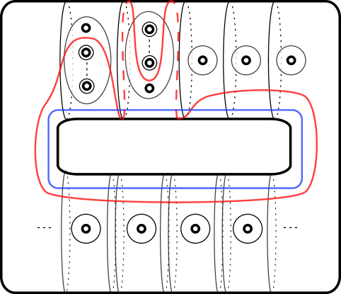
Figure 3. Genus one open book decompositions of the contact manifolds $(Y_{\infty},\xi_{i})$ and $(Y_{n},\eta_{i,j}^{n})$ where $j=l-r$ and $n=l+r+i+2$. The thick circles are the boundary of the page and the label $i$ determines how many times the region along the bottom should be repeated. To get an open book compatible with $(Y_{\infty},\xi_{i})$, take the monodromy as the product of Dehn twists along all curves, except $F$ and $\mathcal{L}_{l,r}$, with signs as indicated. Add a positive twist along the curve $\mathcal{L}_{l,r}$ to get $(Y_{n},\eta_{i,j})$. The curve $F$ is shown for comparison.

Proposition 4.1.

There is a Legendrian link $\mathcal{L}_{l,r}\cup\mathcal{C}$ in $(Y_{\infty},\xi_{i+1})$, for every $i\geq 0$, so that Legendrian surgery along $\mathcal{L}_{l,r}\cup\mathcal{C}$ gives the contact manifold $(Y_{n},\eta_{i,j}^{n})$, while surgery along $\mathcal{L}_{l,r}$ gives the contact manifold $(Y_{n+1},\eta_{i+1,j}^{n+1})$, where $j=l-r$ and $n=l+r+i+2$. For every $i$, the links $\mathcal{L}_{l,r}\cup\mathcal{C}$ are smoothly isotopic in $Y_{\infty}$. Further, the image of $\mathcal{L}_{l,r}$ in $\xi_{i+1}$ under the surgery along $\mathcal{C}$ can be identified with $\mathcal{L}_{l,r}$ in $\xi_{i}$.

We will prove Proposition 4.1 by first constructing open book decompositions compatible with $(Y_{\infty},\xi_{i+1})$ which have the Legendrian knot $F$ sitting naturally on a page, and see how to stabilize $F$ to get the knot $\mathcal{L}_{l,r}$, still sitting on the page of a compatible open book. We then show how to modify this open book by adding positive Dehn twists to its monodromy to get an open book compatible with $\xi_{i}$, noting that this takes the knot $F$ in $\xi_{i+1}$ to the knot $F$ in $\xi_{i}$.

We deal primarily with open books in their abstract form: as a surface $S$ with boundary together with a self-diffeomorphism $\phi$, usually presented as a product of Dehn twists along curves labeled either $+$ or $-$ on a diagram of $S$. In Figure 3, such a diagram is given for the contact manifold $(Y_{\infty},\xi_{i})$. The surface $S$ is a torus with $3i+n+3$ open disks removed. The monodromy consists of positive (right-handed) Dehn twists about circles parallel to (most) boundary circles of $S$ together with negative (left-handed) Dehn twists about certain pairwise disjoint curves which intersect $F$ once. We will call these latter curves meridians. In [26] (see Section 4.4), it was shown how such open books corresponded to torus bundles as well as how these open books could be embedded. We discuss some of that procedure here.

The total space $Y_{\infty}$ is a torus bundle. We can see the bundle structure directly from the open book. Begin by looking at a meridian $c$ on the torus $S$ in Figure 3 which is disjoint from those curves used in the presentation of the monodromy. Since $c$ is fixed by the monodromy, it traces out a torus which will be a fiber in the torus bundle $Y_{\infty}$. As we move $c$ around the torus page it traces out a family of torus fibers. When $c$ crosses the meridional (negative) Dehn twists, this induces a (negative) Dehn twist along the torus fiber, along a curve parallel to the page of the open book. Crossing a boundary circle with a positive Dehn twist induces a negative Dehn twist along the fiber, this time along a direction orthogonal to that of the page (see [26, Section 4.2]). These two Dehn twists correspond to the standard Dehn twist generators of the mapping class group of the torus and allow one to construct all the universally tight, linearly twisting contact structures on torus bundles (i.e. those described in Proposition 2.1).

The region above the bracket labeled ‘$i$ times’ shows an open book compatible with a region of Giroux torsion one (multiplied $i$ times). When $i=0$, the open book describes the unique Stein fillable contact structure (see [26, Section 4.5]). Each of the pieces of the open book swept out as $c$ passes a boundary component is a bypass and is compatible with a linear contact form of type used in Proposition 2.1. The horizontal arcs that make up the curve $F$ in Figure 3 are linear in these local models (see [26, Figure 4.5]) and correspond to a Legendrian $\{pt\}\times I$ in $T^{2}\times I$. Section 4.5 of [26] constructs our particular open books and shows they are compatible with the given contact structures; the manifold $Y_{\infty}$ is the torus bundle with monodromy $T^{-1}S=\left(\begin{array}[]{cc}1&1\\ -1&0\end{array}\right)$. (This is different than what is stated in [26, Section 4.7.2]. The second author gave there a description of the torus bundle with the wrong orientation (0 surgery on the left-handed trefoil).)

We will prove this compatibility later in Proposition 4.6. The first thing we need for Proposition 4.1 is a way to stabilize $F$ on the page of a compatible open book.

2pt $\mathcal{L}$ at 220 80 $\mathcal{L}_{-}$ at 40 155 $\mathcal{L}_{+}$ at 40 25

Figure 4. Local picture of the front projection for two Legendrian stabilizations.

Definition 4.2.

Let $\mathcal{L}$ be a Legendrian knot. There are two stabilizations of $\mathcal{L}$, positive and negative, denoted by $\mathcal{L}_{+}$ and $\mathcal{L}_{-}$, resp., given by the front projections shown in Figure 4.

Oriented to the right as shown in Figure 4, $\mathcal{L}_{-}$ and $\mathcal{L}_{+}$ have

$${\tt rot}(\mathcal{L}_{-}\cup\overline{\mathcal{L}})=-1$$

and

$${\tt rot}(\mathcal{L}_{+}\cup\overline{\mathcal{L}})=+1.$$

Definition 4.3.

Let $L$ be a knot on a page of an open book. There are two stabilizations, left and right, denoted by $L_{l}$ and $L_{r}$, resp., given by the local pictures shown in Figure 5.

$P$ at 27 39 $K_{r}$ at 88 55 $K_{l}$ at 157 23 $K$ at 55 45 $+$ at 73 51 $+$ at 189 29

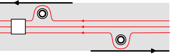
Figure 5. Local picture of the two stabilizations of a knot on a page of an open book. All knots $K$, $K_{l}$ and $K_{r}$ are oriented to the left, so that $K_{l}$ is obtained by sliding $K$ across a trivial stabilization on its left, and similarly $K_{r}$ on its right. The patch $P$ is used in Lemma 4.4 to prove that open book stabilizations give rise to Legendrian stabilizations. The embedded knots $K$, $K_{l}$ and $K_{r}$ are smoothly isotopic.

We need the following lemma and will sketch its proof. A more complete proof can be found in [19].

Lemma 4.4.

Let $K$ be a nonisolating knot on a page of an open book. If $\mathcal{L}$ is the Legendrian realization of $K$, then the Legendrian realization of $K_{r}$ is the negative stabilization $\mathcal{L}_{-}$ and the Legendrian realization of $K_{l}$ is the positive stabilization $\mathcal{L}_{+}$.

Sketch of proof.

First, observe that we can make $K$, $K_{l}$ and $K_{r}$ simultaneously Legendrian while sitting on the same page $\Sigma$ of the open book, and we let $\mathcal{L}$, $\mathcal{L}_{l}$ and $\mathcal{L}_{r}$ refer to these Legendrian knots. All three knots are smoothly isotopic and so $K\cup\overline{K}_{l}$ bounds an annulus, $A$. We can make this annulus convex with Legendrian boundary $\mathcal{L}\cup\overline{\mathcal{L}}_{l}$, starting with the patch $P$ as shown in Figure 5, a subset of the page. Since the dividing set is empty on $\Sigma$, it is empty on $P$ and so the dividing set of $A$ consists of boundary parallel arcs adjacent to $K_{l}$. Comparing framings shows that there is only one such arc and so ${\tt rot}(K\cup\overline{K}_{l})=\xi(A_{+})-\xi(A_{-})=-1=-{\tt rot}(K_{l}\cup\overline{K})$. This shows that $K_{l}$ is the positive stabilization. ∎

We will also need the following tool regarding stabilizations of open books.

Lemma 4.5 (The braid relation).

Two open books which locally differ as in Figure 6 are related by a positive Hopf stabilization. There is a contact structure $\xi$ defined in a neighborhood of the local picture compatible with both open books and such that the horizontal arc $K$ is Legendrian and sitting on a page in each.

           

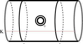
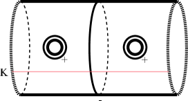
Figure 6. Local pictures $B_{1}$ and $B_{2}$ of open books which differ by a Hopf stabilization.

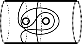
2pt $\sigma_{1}$ at 131 95 $\sigma_{2}$ at 38 100 $\sigma_{3}$ at 93 7              $\partial_{1}$ at 116 42 $\partial_{2}$ at 64 42 $\partial_{3}$ at 27 5 $\partial_{4}$ at 166 5

Figure 7. The lantern relation

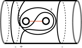
Figure 8. The monodromy of $B_{2}$ after applying the lantern relation. The obvious destabilizing arc is shown.

Proof.

The lantern relation (shown in Figure 7) relates the product of right-handed Dehn twists along each boundary component to the product of those along the three interior curves: $\partial_{1}\partial_{2}\partial_{3}\partial_{4}=\sigma_{1}\sigma_{2}\sigma_{3}$, (where the Dehn twists act left to right). This diagram is different than the usual presentation of the lantern relation which draws the surface as a three-holed disk with the curves $\sigma_{i}$ placed symmetrically, cf. [1, 16], but is more convenient for our purposes here.

The segment $B_{2}$ of the open book shown on the right hand side of Figure 6 is a 4-holed sphere with monodromy $\partial_{1}\partial_{2}\sigma_{3}^{-1}$ using the same curves as in Figure 7. After applying the lantern relation to $B_{2}$ we get the presentation $\sigma_{1}\sigma_{2}\partial_{3}^{-1}\partial_{4}^{-1}$. In applying the lantern relation here it is important that all $\partial_{i}$ commute with each other and with all $\sigma_{i}$. The new presentation is shown in Figure 8 with an obvious destabilizing arc. After destabilizing, we are left with the open book segment $B_{1}$. Notice that the destabilizing arc is disjoint from the horizontal arc $K$ shown in Figure 6 and so we can apply the braid relation even when there are Dehn twists along curves running parallel to the segment, so long as the Dehn twists along $\partial_{1}$ and $\partial_{2}$ occur simultaneously in the described factorization. It was shown in [26, Section 4.2] how to construct a contact form compatible with $B_{1}$. Gluing two of these together gives a contact form compatible with both $B_{2}$ and $B_{1}$ and with the horizontal arc $K$ being Legendrian and sitting on pages of each. ∎

Proposition 4.6.

The open books described in Figure 3 are compatible with the contact structures $\xi_{i}$ on $Y_{\infty}$ with the Legendrian knot $F$ from Proposition 2.1 sitting on the page as the knot $F$ in the figure.

Proof.

This can and is proved without resorting to many of the intricacies discussed in the beginning of the section. We first note that the region labeled $i$ times is a region of Giroux torsion 1, multiplied $i$ times, and for convenience, let us denote the associated open book $\mathfrak{B}_{i}$. From [26, Lemma 4.4.4] and its corollary, we see that the compatible contact structures are weakly fillable for all $i$ and hence by the classification in [10, 14] must be in the Giroux’s family of tight contact structures constructed in Section 2.1. From [26, Section 4.5] — recalling that the monodromy for the right-handed trefoil is $T^{-1}S=\left(\begin{array}[]{cc}1&1\\ -1&0\end{array}\right)$ — we see that, when $i=0$, the compatible contact structure has zero Giroux torsion. (Indeed, it can be realized by Legendrian surgery on the Stein fillable contact structure on $T^{3}$). Thus $\mathfrak{B}_{i}$ is compatible with $\xi_{i}$. To see that the curve $F$ in the diagram really is the Legendrian $F$ discussed after Proposition 2.1, we do need a bit of detail. Looking at [26, Figure 4.5], the embedded diagram of a basic slice is compatible with a linearly twisting contact form of the type discussed in Proposition 2.1, and further the arc tangent to the $t$-axis at the left and right sides of the picture is Legendrian. One can glue any number of basic slices together (as well as gluing the front and back boundaries together) and the resulting open book will still be compatible with a linear contact form and the matched horizontal arc will remain Legendrian. ∎

Proof of Proposition 4.1.

From Proposition 4.6 and Lemma 4.4 we see that $\mathcal{L}_{l,r}$ is $F_{i,j}$ from Section 2.1, (where $j=l-r$ and $n=l+r+i+2$). Thus adding a right handed Dehn twist to the open book along $\mathcal{L}_{l,r}$ gives an open book compatible with $(Y_{n},\eta_{i,j}^{n})$ and this describes the surgery from $Y_{\infty}$ to $Y_{n}$.

To find the second link $\mathcal{C}$ and prove the lemma, we add positive twists to the monodromy of $(Y_{\infty},\xi_{i+1})$ in a small standard region of a compatible open book and see that, after applying the braid relation of Lemma 4.5, we have an open book compatible with $(Y_{\infty},\xi_{i})$. Notice now that each open book for $(Y_{\infty},\xi_{i+1})$, $i\geq 0$, has a region:

which describes a region of Giroux torsion one plus a basic slice. To this, we add positive twists to the monodromy to get to the following open book.

These positive twists make up the Legendrian link $\mathcal{C}$. Now repeatedly apply the braid relation and reduce to the open book for $(Y_{\infty},\xi_{i})$ where the Giroux torsion has been excised. Locally we now have the following picture.

Since the braid relation can be applied in the presence of Dehn twists along a horizontal curve (i.e. the red curve in the pictures above, see Figure 6), attaching Stein handles along $\mathcal{L}_{l,r}\cup\mathcal{C}$ in $(Y_{\infty},\xi_{i+1})$ gives an open book which is related to that shown in Figure 3 for $(Y_{n},\eta_{i,j}^{n})$ by Hopf stabilization. We showed in Lemma 4.5 that the braid relation does not change how horizontal knots on the page are embedded up to an ambient contact isotopy, and thus after surgery and applying braid relation the image of the Legendrian knot $\mathcal{L}_{l,r}$ from $\xi_{i+1}$ sits on a page of the open book as $\mathcal{L}_{l,r}$ in $\xi_{i}$. ∎

4.2. The computation of the invariants

Lemma 4.7.

All tight contact structures $\xi_{i}$ on $Y_{\infty}$ are homotopic and have $3$-dimensional homotopy invariant $\theta(\xi_{i})=-4$

Proof.

The homotopy between all the contact structures $\xi_{i}$ was proved in [9, Proposition 2]. Therefore we can compute the $3$-dimensional homotopy invariant of $\xi_{0}$, which has a Stein filling $(V_{\infty},J_{\infty})$ obtained by attaching a Stein handle on a Legendrian right-handed trefoil knot with Thurston–Bennequin invariant $0$ (see Figure 1). It is easy to see that $c_{1}(J_{\infty})=0$, $\chi(V_{\infty})=2$, and $\sigma(V_{\infty})=0$. The formula for the $3$-dimensional homotopy invariant in [11, Definition 4.2] is

$$\theta(\xi_{0})=c_{1}(J_{\infty})^{2}-2\chi(V_{\infty})-3\sigma(V_{\infty}),$$

so $\theta(\xi_{0})=-4$. ∎

Lemma 4.8 ([5, Theorem 3.12]).

All tight contact structures $\eta_{i,j}^{n}$ are homotopic and have $3$-dimensional homotopy invariant $\theta(\xi_{i})=-6$.

The reference [5] computes $\frac{\theta}{4}$ for $i=0$ or $i=n$, but the proof can be extended to all cases without modification.

Lemma 4.9.

$\underline{\widehat{HF}}(-Y_{\infty})\cong\mathbb{Z}[H^{1}(-Y_{\infty})]\oplus\mathbb{Z}[H^{1}(-Y_{\infty})]$ with one summand in degree $\frac{1}{2}$ and one in degree $\frac{3}{2}$. Moreover $c(\xi_{0})$ is a generator of the summand in degree $\frac{1}{2}$.

Proof.

$-Y_{\infty}$ can be obtained by $0$-surgery on the left-handed trefoil knot and the Poincaré sphere $\Sigma(2,3,5)$ can be obtained by $(-1)$-surgery on the same knot. Then the surgery exact triangle of Theorem 3.2 gives:

where the horizontal map $F$ is induced by a cobordism $W$ constructed by the attachment of a $2$-handle with framing $-1$ along the left-handed trefoil knot. Therefore the integer homology group $H_{2}(W)$ is generated by a surface $\widehat{\Sigma}$ with self-intersection $\widehat{\Sigma}^{2}=-1$. The ${\rm Spin}^{c}$-structures on $W$ are indexed by integers $k$ such that $\langle c_{1}(\mathfrak{s}_{k}),[\widehat{\Sigma}]\rangle=2k+1$, so $c_{1}(\mathfrak{s}_{k})^{2}=-(2k+1)^{2}$. By Theorem 3.2, $F=\sum\limits_{k\in\mathbb{Z}}F_{W,\mathfrak{s}_{k}}\otimes t^{k}$. For any ${\rm Spin}^{c}$-structure $\mathfrak{s}_{k}$ the map $F_{W,\mathfrak{s}_{k}}$ shifts the degree by

$$\frac{1}{4}\left(c_{1}(\mathfrak{s}_{k})^{2}-2\chi(W)-3\sigma(W)\right)=-k(k+1).$$

Since $-k(k+1)\leq 0$, $\widehat{HF}(S^{3})\cong\mathbb{Z}_{(0)}$ and $\widehat{HF}(\Sigma(2,3,5))\cong\mathbb{Z}_{(2)}$, the horizontal map is trivial. This implies that $\underline{\widehat{HF}}(-Y_{\infty})\cong\mathbb{Z}[H^{1}(-Y_{\infty})]\oplus\mathbb{Z}[H^{1}(-Y_{\infty})]$. The second homology group of $Y_{\infty}$ is generated by an embedded torus, and therefore the adjunction inequality [22, Theorem 7.1], which holds also for Heegaard Floer homology with twisted coefficients, implies that $\underline{\widehat{HF}}(-Y_{\infty})$ is concentrated in the trivial ${\rm Spin}^{c}$-structure.

The Heegaard Floer homology groups for ${\rm Spin}^{c}$-structures with torsion first Chern class admit an absolute $\mathbb{Q}$-grading [24, Section 7], which we are now going to determine for $\underline{\widehat{HF}}(-Y_{\infty})$. The map $\widehat{HF}(\Sigma(2,3,5))[t,t^{-1}]\to\underline{\widehat{HF}}(-Y_{\infty})$ is induced by a $2$-handle attachment. The first Betti number of $\Sigma(2,3,5)$ is smaller than the first Betti number of $Y_{\infty}$, so the handle is attached along a null-homologous knot with framing $0$. Then the induced map has degree $-\frac{1}{2}$.

The map $\underline{\widehat{HF}}(-Y_{\infty})\to\widehat{HF}(S^{3})[t,t^{-1}]$ is induced by a $2$-handle attachment along a homologically nontrivial knot, so it also has degree $-\frac{1}{2}$; see for example [20, Lemma 3.1]. This implies that

$$\underline{\widehat{HF}}(-Y_{\infty})\cong\mathbb{Z}[H^{1}(-Y_{\infty})]\oplus\mathbb{Z}[H^{1}(-Y_{\infty})],$$

with one summand in degree $\frac{3}{2}$ and the other one in degree $\frac{1}{2}$.

The contact invariant $c(\xi_{0})$ has degree $-\frac{\theta(\xi_{0})}{4}-\frac{1}{2}=\frac{1}{2}$ and is a generator of $\underline{\widehat{HF}}_{1/2}(-Y_{\infty})$ by [21, Theorem 4.2]. ∎

Lemma 4.10 ([25, Section 3]).

For any $n\geq 2$, $\widehat{HF}_{+1}(-Y_{n})\cong\mathbb{Z}^{n-1}$ and the contact invariants $c(\eta_{0,-n+2}^{n}),\ldots,c(\eta_{0,n-2}^{n})$ form a basis.

The surgery described in Proposition 4.1 produces a cobordism $Z_{n}$ from $Y_{\infty}$ to $Y_{n}$ which can be decomposed in two different ways:

• either as a cobordism $W_{\infty}$ from $Y_{\infty}$ to itself followed by a cobordism $V_{n}$ from $Y_{\infty}$ to $Y_{n}$ if we attach $2$-handles along ${\mathcal{C}}$ first, and then along ${\mathcal{L}}$,

• or as a cobordisms $V_{n+1}$ from $Y_{\infty}$ to $Y_{n+1}$ followed by a cobordism $W_{n}$ from $Y_{n+1}$ to $Y_{n}$ if we attach $2$-handles along ${\mathcal{L}}$ first, and then along ${\mathcal{C}}$.

These cobordisms induce maps on Heegaard Floer homology according to Theorem 3.1. Now we compute the change of the coefficient group for the maps induced by the cobordisms above. Let $K(V_{n})=\ker\left(H^{2}(V_{n},Y_{\infty})\to H^{2}(V_{n})\right)$. By the cohomology exact sequence the map $H^{1}(Y_{\infty})\to H^{2}(V_{n},Y_{\infty})$ is an isomorphism. Therefore $K(V_{n})\cong H^{1}(Y_{\infty})$ and we can identify $\mathbb{Z}[K(V_{n})]$ with $\mathbb{Z}[H^{1}(Y_{\infty})]$. Here we have used the fact that $Y_{n}$ is an integer homology sphere. The manifolds $Y_{n}$ are integer homology spheres, so the groups $K(W_{n})$ are trivial. Moreover $H^{2}(Z_{n},\partial Z_{n})=H^{2}(W_{n},\partial W_{n})\oplus H^{2}(V_{n+1},\partial V_{n+1})$ and $H^{2}(Z_{n})=H^{2}(W_{n})\oplus H^{2}(V_{n+1})$, so $K(Z_{n})\cong K(W_{n})\oplus K(V_{n+1})\cong K(V_{n+1})$.

Lemma 4.11.

The connecting homomorphism $\delta\colon H^{1}(Y_{\infty})\to H^{2}(Z_{n})$ in the Mayer–Vietoris exact sequence for the decomposition $Z_{n}=W_{\infty}\cup_{Y_{\infty}}V_{n}$ is the trivial map.

Proof.

It is easier to see this by taking the Poincaré–Lefschetz duals and looking at the associated map in the Mayer–Vietoris exact sequence for relative homology. There $\delta\colon H^{1}(Y_{\infty})\to H^{2}(Z_{n})$ becomes $i\colon H_{2}(Y_{\infty})\to H_{2}(Z_{n},\partial Z_{n})$. This map is trivial because the torus generating $H_{2}(Y_{\infty})$ is homologous (indeed isotopic) to the torus generating the second homology group of the copy of $Y_{\infty}$ in the boundary of $Z_{n}$. This can be seen by examining $W_{\infty}$, which is built from $Y_{\infty}$ by adding 2-handles along curves, each lying on a torus fiber. Hence the torus fibers in each boundary component of $W_{\infty}$ are isotopic. ∎

Lemma 4.11 and Lemma 3.3 imply that $K(V_{n})(W_{\infty})\cong K(Z_{n})$, so also $\mathbb{Z}[K(W_{\infty})]\cong\mathbb{Z}[H^{1}(Y_{\infty})]$. Moreover the cobordism $W_{\infty}$ satisfies the hypotheses of Lemma 3.8. By Theorem 3.1 and Lemma 3.8, $V_{n}$ and $W_{\infty}$ induce maps

$$F_{V_{n},\mathfrak{k}}\colon\widehat{HF}(-Y_{n})\to\underline{\widehat{HF}}(-Y_{\infty})\quad\text{and}\quad F_{W_{\infty},\mathfrak{k}}\colon\underline{\widehat{HF}}(-Y_{\infty})\to\underline{\widehat{HF}}(-Y_{\infty}),$$

where the map $F_{W_{\infty},\mathfrak{k}}$ is $\mathbb{Z}[H^{1}(Y_{\infty})]$-linear. By an abuse of notation, we will denote the canonical ${\rm Spin}^{c}$-structure on a symplectic cobordism by $\mathfrak{k}$ regardless of what the cobordism or the symplectic form are; in fact this will not be very important in our proof. These maps fit into a diagram:

(5)

which commutes for a suitable choice of the maps in their equivalence class, because Lemma 4.11 implies that the restriction map $\mathfrak{s}\mapsto(\mathfrak{s}|_{W_{\infty}},\mathfrak{s}|_{V_{n}})$ gives an isomorphism ${\rm Spin}^{c}(Z_{n})\cong{\rm Spin}^{c}(W_{\infty})\times{\rm Spin}^{c}(V_{n})$, and we have a similar isomorphism ${\rm Spin}^{c}(Z_{n})\cong{\rm Spin}^{c}(V_{n+1})\times{\rm Spin}^{c}(W_{n})$ because $H^{1}(Y_{n})=0$.

From now on we will make a change in the coefficient ring which will allow us to write our formulas in a more symmetric form. Let $\Lambda=\mathbb{Z}[H^{1}(Y_{\infty},\frac{1}{2}\mathbb{Z})]$ with the $\mathbb{Z}[H^{1}(Y_{\infty})]$-module structure defined by the inclusion $H^{1}(Y_{\infty})\subset H^{1}(Y_{\infty},\frac{1}{2}\mathbb{Z})$. Since $\Lambda$ is a free module over $\mathbb{Z}[H^{1}(Y_{\infty})]$, we have

$$\underline{\widehat{HF}}(-Y_{\infty};\Lambda)\cong\underline{\widehat{HF}}(-Y_{\infty})\otimes_{\mathbb{Z}[H^{1}(-Y_{\infty})]}\Lambda\cong\Lambda_{\left(\frac{1}{2}\right)}\oplus\Lambda_{\left(\frac{3}{2}\right)}.$$

We choose an identification $\underline{\widehat{HF}}_{\frac{1}{2}}(-Y_{\infty};\Lambda)\cong\Lambda$ such that $[c(\xi_{0})]$ corresponds to $[1]$.

Lemma 4.12.

We can choose a representative of $F_{V_{n}}$, an identification of $\underline{\widehat{HF}}_{(\frac{1}{2})}(-Y_{\infty};\Lambda)$ with $\mathbb{Z}[t^{\pm\frac{1}{2}}]$, and signs for the contact invariants $c(\eta_{0,j})$ such that

$$F_{V_{n},\mathfrak{k}}(c(\eta_{0,j}^{n}))=t^{j/2}.$$

Proof.

Let us view the $4$-manifold $V_{\infty}$ used in the proof of Lemma 4.7, constructed by adding a $2$-handle to $D^{4}$ along the right-handed trefoil knot in Figure 1 with attaching framing $0$, as a cobordism from $S^{3}$ to $Y_{\infty}$ and let $X_{n}=V_{\infty}\cup_{Y_{\infty}}V_{n}$. The second homology group of $X_{n}$ is generated by the class $T$ of a torus fiber in $Y_{\infty}$ and by the class of a sphere $S$ such that $S\cdot T=1$.

Let $\mathfrak{s}_{j}$ be the ${\rm Spin}^{c}$-structure on $X_{n}$ such that

$$\langle c_{1}(\mathfrak{s}_{j}),T\rangle=0\quad\text{and}\quad\langle c_{1}(\mathfrak{s}_{j}),S\rangle=j\text{ with }j\equiv n(\text{ mod }2).$$

The restriction of all the ${\rm Spin}^{c}$-structures $\mathfrak{s}_{j}$ to $V_{\infty}$ and $V_{n}$ coincide, so there is a generator $h$ of $H^{1}(Y_{\infty})$ such that $\mathfrak{s}_{j+2}=\mathfrak{s}_{j}+\delta(h)$.

We denote $\mathfrak{s}_{j}|_{V_{\infty}}=\mathfrak{h}$, $\mathfrak{s}_{j}|_{V_{n}}=\mathfrak{k}$ (in fact one can verify that the ${\rm Spin}^{c}$-structure $\mathfrak{s}_{j}|_{V_{n}}$ coincide with the ${\rm Spin}^{c}$-structure in Diagram (5)) and identify $\Lambda$ with $\mathbb{Z}[t^{\pm 1/2}]$ by sending $e^{h}$ to $t$. By the composition formula in Theorem 3.4 we can choose $F_{V_{n},\mathfrak{k}}$ such that

$$F_{X_{n},\mathfrak{s}_{j}}=\Pi\circ F_{V_{\infty},\mathfrak{h}}\circ t^{-j/2}\cdot F_{V_{n},\mathfrak{k}}.$$

In fact we choose $F_{V_{n},\mathfrak{k}}$ such that $F_{X_{n},\mathfrak{s}_{-n}}=\Pi\circ F_{V_{\infty},\mathfrak{h}}\circ t^{n/2}\cdot F_{V_{n},\mathfrak{k}}$ and the formula follows from Equation (4) because $\mathfrak{s}_{j}=\mathfrak{s}_{-n}+\frac{j+n}{2}\delta(h)$.

The restriction map $H^{2}(V_{\infty};\mathbb{Z})\to H^{2}(Y_{\infty};\mathbb{Z})$ is an isomorphism and $H^{1}(V_{\infty})=0$, so $K(V_{\infty})\cong H^{1}(Y_{\infty})$, and then $V_{\infty}$ induces an anti-$\Lambda$-linear map

$$F_{V_{\infty}}\colon\underline{\widehat{HF}}(-Y_{\infty};\Lambda)\to\widehat{HF}(S^{3})[t^{1/2},t^{-1/2}].$$

Since the right-handed trefoil knot has a Legendrian representative with Thurston–Bennequin invariant $+1$, $V_{\infty}$ can be endowed with a Stein structure providing a Stein cobordism from $(S^{3},\xi_{st})$ to $(Y_{\infty},\xi_{0})$ with canonical ${\rm Spin}^{c}$-structure $\mathfrak{h}$, so $[F_{V_{\infty},\mathfrak{h}}(c(\xi_{0}))]=[c(\xi_{st})]$. Then, after identifying both $\underline{\widehat{HF}}_{\frac{1}{2}}(-Y_{\infty};\Lambda)$ and $\widehat{HF}(S^{3})[t^{1/2},t^{-1/2}]$ with $\mathbb{Z}[t^{\pm 1/2}]$, we can choose $F_{V_{\infty},\mathfrak{h}}$ to be the conjugation map $t\mapsto t^{-1}$.

The ${\rm Spin}^{c}$-structure $\mathfrak{s}_{j}$ on $X_{n}$ is the canonical ${\rm Spin}^{c}$-structure of the Stein filling $(X_{n},J_{n})$ of $\eta_{0,j}^{n}$ described by the Legendrian surgery diagram in Figure 9. Then we know from [25] that $F_{X_{n},\mathfrak{s}_{j}}(c(\eta_{0,j}^{m}))=c(\xi_{st})$, and $F_{X_{n},\mathfrak{s}_{k}}(c(\eta_{0,j}^{n}))=0$ for $k\neq j$. Using the composition formula in Theorem 3.4 and the fact that $F_{V_{\infty},\mathfrak{h}}$ is, in our choice of identifications, the conjugation map, we conclude that $F_{V_{n},\mathfrak{k}}(c(\eta_{0,j}^{n}))=t^{j/2}$. ∎

\psfrag{a}{\footnotesize$\frac{n-j}{2}$ cusps}\psfrag{b}{\footnotesize$\frac{n+j}{2}$ cusps}\includegraphics[width=170.71652pt]{nodoleg}

Figure 9. Legendrian surgery presentation of $(Y_{n},\eta_{0,j}^{n})$.

Now we choose the maps in Diagram (5) so that it becomes commutative. The horizontal map in the upper part is fixed because the $Y_{n}$ are integer homology spheres, while the vertical maps are fixed by the choices in Lemma 4.12.

Lemma 4.13.

If we choose $F_{V_{n},\mathfrak{k}}$ such that $F_{V_{n},\mathfrak{k}}(c(\eta_{0,j}^{n}))=t^{j/2}$ for all $n$, then Diagram (5) commutes if we choose the map $F_{W_{\infty},\mathfrak{k}}$ to be represented by the multiplication by $t^{\frac{1}{2}}-t^{-\frac{1}{2}}$.

Proof.

The contact structure $\xi_{1}$ is obtained from $\xi_{0}$ by a generalized Lutz twist, so $[c(\xi_{1})]=[(t-1)c(x_{0})]$ by [6, Theorem 2]. This implies that $F_{W_{\infty},\mathfrak{k}}$ is the multiplication by $(t-1)t^{k/2}$ for some $k\in\mathbb{Z}$. We will now determine which choice for $F_{W_{\infty},\mathfrak{k}}$ will make Diagram (5) commutative.

Inverting the orientation of the contact planes results in a symmetry of the triangle (1) about its vertical axis. In particular the contact structure $\eta_{n-2,0}^{n}$ is invariant under conjugation, and $\eta_{0,j}^{n}$ is conjugated to $\eta_{0,-j}^{n}$; see [4, Proposition 3.8], where $\eta_{n-2,0}^{n}$ is called $\eta_{0}$, and $\eta_{0,j}^{n}$ is called $\eta_{j}$. In the reference only odd $n$ are considered, but the proof carries through in general. By Lemma 4.10 we know that $c(\eta_{n-2,0}^{n})$ can be expressed as a linear combination of the elements $c(\eta_{0,i}^{n})$. The invariance of $c(\eta_{n-2,0}^{n})$ by conjugation implies that $c(\eta_{n-2,0}^{n})=a_{1-n}c(\eta_{0,1-n}^{n})+\ldots+a_{n-1}c(\eta_{0,n-1}^{n})$ with $a_{j}=a_{-j}$. hence $F_{V_{n},\mathfrak{k}}(c(\eta_{n-2,0}^{n}))$ is a symmetric Laurent polynomial in the variable $t^{1/2}$ because it is invariant under the automorphism $t^{1/2}\mapsto t^{-1/2}$.

Since $F_{V_{n+1},\mathfrak{k}}(c(\eta_{n-2,0}^{n}))=c(\eta_{n-1,0}^{n+1})$, the composite $F_{V_{n+1},\mathfrak{k}}\circ F_{W_{n},\mathfrak{k}}$ maps $c(\eta_{n-2,0}^{n})$ to a symmetric Laurent polynomial. If Diagram (5) commutes, then $F_{W_{\infty},\mathfrak{k}}$ maps symmetric Laurent polynomials to symmetric Laurent polynomials and therefore it must be the multiplication by $t^{1/2}-t^{-1/2}$. ∎

Proof of Theorem 1.3.

The theorem will be proved by induction on $n$. The initial step is $n=2$. Since there is a unique tight contact structure on $Y_{2}$ by [8, Theorem 4.9], there is nothing to prove in this case. Now we assume that Formula (2) holds for the tight contact structures on $Y_{n}$, for some $n$, and we prove that this implies that Formula (2) holds for the tight contact structures on $Y_{n+1}$. From the surgery construction we have

$$F_{W_{n},\mathfrak{k}}(c(\eta_{i,j}^{n}))=c(\eta_{i+1,j}^{n+1}),$$

and the induction hypothesis gives, on $Y_{n+1}$, the following expression for the contact invariants of $\eta_{i,j}^{n+1}$ for $i\geq 1$ in terms of the contact invariants of $\eta_{1,j}^{n+1}$:

(6) $$c(\eta_{i+1,j}^{n+1})=\sum\limits_{k=0}^{i}(-1)^{k}\binom{i}{k}c(\eta_{1,j-i+2k}^{n+1}).$$

We can compute $c(\eta_{1,j}^{n+1})$ by the the commutativity of Diagram 5: in fact

$$F_{V_{n+1},\mathfrak{k}}(c(\eta_{1,j}^{n+1}))=F_{W_{\infty},\mathfrak{k}}(F_{V_{n},\mathfrak{k}}(c(\eta_{0,j}^{n})))=t^{(j+1)/2}-t^{(j-1)/2},$$

and therefore

(7) $$c(\eta_{1,j}^{n+1})=c(\eta_{0,j+1}^{n+1})-c(\eta_{0,j-1}^{n+1})$$

because the map $F_{V_{n+1},\mathfrak{k}}$ is injective.

If we substitute $c(\eta_{1,j}^{n+1})$ in Equation 6 with the right-hand side of Equation 7, and write $j-i+1+2k=j-(i+1)+2(k+1)$, we obtain:

$$c(\eta_{i+1,j}^{n+1})=\sum\limits_{k=0}^{i}(-1)^{k}\binom{i}{k}(c(\eta_{0,j-(i+1)+2(k+1)}^{n+1})-c(\eta_{0,j-(i+1)+2k}^{n+1}))$$

$$=\sum\limits_{k=1}^{i+1}(-1)^{k-1}\binom{i}{k-1}c(\eta_{0,j-(i+1)+2k}^{n+1})-\sum\limits_{k=0}^{i}(-1)^{k}\binom{i}{k}c(\eta_{0,j-(i+1)+2k}^{n+1})$$

$$=\sum\limits_{k=0}^{i+1}(-1)^{k-1}\left[\binom{i}{k}+\binom{i}{k-1}\right]c(\eta_{0,j-(i+1)+2k}^{n+1})$$

$$=\sum\limits_{k=0}^{i+1}(-1)^{k-1}\binom{i+1}{k}c(\eta_{0,j-(i+1)+2k})$$

from which the statement of Theorem 1.3 follows. ∎

References

- [1] M. Dehn. Die Gruppe der Abbildungsklassen. Acta Math., 69(1):135–206, 1938.
- [2] J. Etnyre and K. Honda. On the nonexistence of tight contact structures. Ann. of Math. (2), 153(3):749–766, 2001.
- [3] P. Ghiggini. Strongly fillable contact 3-manifolds without Stein fillings. Geom. Topol., 9:1677–1687, 2005.
- [4] P. Ghiggini. Infinitely many universally tight contact manifolds with trivial Ozsváth-Szabó contact invariants. Geom. Topol., 10:335–357, 2006.
- [5] P. Ghiggini. Ozsváth-Szabó invariants and fillability of contact structures. Math. Z., 253(1):159–175, 2006.
- [6] P. Ghiggini and K. Honda. Giroux torsion and twisted coefficients. arXiv:0804.1568.
- [7] P. Ghiggini, K. Honda and J. Van Horn-Morris. The vanishing of the contact invariant in the presence of torsion. arXiv:0706.1602
- [8] P. Ghiggini and S. Schönenberger. On the classification of tight contact structures. In Topology and Geometry of Manifolds, volume 71 of Proceedings of Symposia in Pure Mathematics, pages 121–151. American Mathematical Society, 2003.
- [9] E. Giroux. Une infinité de structures de contact tendues sur une infinité de variétés. Invent. Math., 135(3):789–802, 1999.
- [10] E. Giroux. Structures de contact en dimension trois et bifurcations des feuilletages de surfaces. Invent. Math., 141(3):615–689, 2000.
- [11] R. Gompf. Handlebody construction of Stein surfaces. Ann. of Math. (2), 148(2):619–693, 1998.
- [12] M. Greenberg and J. Harper. Algebraic topology. A first course. Mathematics Lecture Note Series, 58. Benjamin/Cummings Publishing Co., Inc., Advanced Book Program, Reading, Mass. 1981.
- [13] K. Honda. On the classification of tight contact structures I. Geom. Topol., 4:309–368, 2000.
- [14] K. Honda. On the classification of tight contact structures II. J. Differential Geom., 55(1):83–143, 2000.
- [15] S. Jabuka and T. Mark. Product formulae for Ozsváth-Szabó 4-manifold invariants. Geom. Topol., 12(3):1557–1651, 2008.
- [16] D. Johnson. Homeomorphisms of a surface which act trivially on homology. Proc. Amer. Math. Soc. 75(1):119–125, 1979.
- [17] P. Lisca and G. Matić. Tight contact structures and Seiberg-Witten invariants. Invent. Math., 129(3):509–525, 1997.
- [18] P. Lisca and A. Stipsicz. Ozsváth-Szabó invariants and tight contact three-manifolds. I. Geom. Topol., 8:925–945, 2004.
- [19] S. Onaran. Legendrian knots and open book decompositions. Ph. D. Thesis, Middle East Technical University, 2009.
- [20] P. Ozsváth and Z. Szabó. Absolutely graded Floer homologies and intersection forms for four-manifolds with boundary. Adv. Math., 173(2):179–261, 2003.
- [21] P. Ozsváth and Z. Szabó. Holomorphic disks and genus bounds. Geom. Topol., 8:311–334, 2004.
- [22] P. Ozsváth and Z. Szabó. Holomorphic disks and three-manifold invariants: properties and applications. Ann. of Math. (2), 159(3):1159–1245, 2004.
- [23] P. Ozsváth and Z. Szabó. Heegaard Floer homology and contact structures. Duke Math. J., 129(1):39–61, 2005.
- [24] P. Ozsváth and Z. Szabó. Holomorphic triangles and invariants for smooth four-manifolds. Adv. Math., 202(2):326–400, 2006
- [25] O. Plamenevskaya. Contact structures with distinct Heegaard Floer invariants. Math. Res. Lett., 11(4):547–561, 2004.
- [26] J. Van Horn-Morris. Contructions of open book decompositions. Ph. D. dissertation, University of Texas at Austin, 2007.
- [27] H. Wu. On Legendrian surgeries. Math. Res. Lett., 14(3):513–530, 2007.