Reconstructions in Ultrasound Modulated Optical Tomography

Abstract

We introduce a mathematical model for ultrasound modulated optical tomography and present a simple reconstruction scheme for recovering the spatially varying optical absorption coefficient from scanning measurements with narrowly focused ultrasound signals. Computational results for this model show that the reconstruction of sharp features of the absorption coefficient is possible. A formal linearization of the model leads to an equation with a Fredholm operator, which explains the stability observed in our numerical experiments.

1 Introduction

During the last two decades, optical tomography (OT) has received significant attention as a biomedical imaging modality. This can be attributed, in particular, to the fact that light at optical frequencies is harmless to the human organism and that optical properties of tissues reveal important biological information such as angiogenesis and hypermetabolism, both of which are well-known indicators of cancer [1]. Unfortunately, reconstruction in OT is also known to be severely ill-posed, and consequently the sharp imaging of optical properties is all but impossible. Various attempts to address this problem have been made. In this paper we are interested in a hybrid imaging method called Ultrasound Modulated Optical Tomography (UOT, [1]) that combines the OT procedure with simultaneous modulation by a narrowly focused ultrasound beam in order to alleviate the instability of OT reconstructions. The idea is to combine the good tumor specificity of OT with the high spatial resolution of ultrasound imaging. This approach utilizes the experimentally observed interaction between ultrasound and light propagation in tissue [2, 1]. In UOT, a coherent light source irradiates the tissue sample and causes interference patterns to form on the surface of the object, so-called speckles. A narrowly focused ultrasound wave is simultaneously induced in the tissue, influencing its optical properties and thus modulating the speckle pattern with ultrasound frequency. By measuring properties of this modulation, information about the incident light intensity at the focus location of the ultrasound beam can be obtained. Hence, by scanning the focus of the ultrasound wave throughout the sample, a quantity related to the light intensity in the object’s interior can be determined. This type of internal information is usually not available from OT measurements due to multiple scattering of photons in optically dense media, although there are other variants of optical tomography that also strive to recover this information (e.g. [3]). It can be expected that this additional knowledge can help in stabilizing the inversion process and render it substantially less ill-posed than the original OT problem. For the UOT model we present in this paper, numerical experiments and an initial analysis suggest that this intuition is justified.

The literature contains a number of models that address the UOT technique, see for example [2, 4, 5, 6, 7, 1]. Most of them describe the coupling between ultrasound and light in terms of stochastic quantities, which permits particle-based simulations of the light intensity modulation effect caused by the ultrasound wave. On the other hand, for optical imaging in turbid media at a depth of several centimeters, photon intensities can be accurately modeled by the diffusion limit. Under certain assumptions, this allows us to formulate a model for the UOT procedure based on a parameter identification problem for a set of coupled diffusion-type partial differential equations. This model, along with a description of the measurements is presented in Section 2. In Section 3, we outline a simple algorithm that can be used to reconstruct the spatially varying absorption coefficient from UOT measurements with focused ultrasound signals. Examples of the resulting reconstructions for numerical phantoms are provided in Section 4. In Section 5, we formally linearize our model and obtain an equation that relates perturbations in the absorption coefficient to those in the measurements by a Fredholm operator acting between appropriate Sobolev spaces. This provides a partial explanation to the stable reconstruction observed in our numerical experiments. The last section contains final remarks and conclusions.

2 Mathematical model

A detailed description of the physical underpinnings of the UOT procedure can be found, for instance, in [1, Ch. 13]. We give a brief description of the set-up here.

Let the object of interest occupy the domain $\Omega\subset{\mathbb{R}}^{3}$. The internal optical properties in the diffusion limit are described by the reduced scattering coefficient $\mu_{s}^{\prime}$ and the absorption coefficient $\mu_{a}$. For imaging soft tissues, it is common to assume $\mu_{s}^{\prime}$ roughly equal to a known constant throughout $\Omega$, while the spatially varying absorption $\mu_{a}(x)$, $x\in\Omega,$ represents the target of reconstruction. It is also assumed that the tissue of interest is turbid (highly scattering), so that $\mu_{a}(x)\ll\mu_{s}^{\prime}$. It is known that in such media, the light intensity $u(x)$ inside $\Omega$ can be accurately described by the diffusion approximation (e.g., [8, 3]).

It has been shown experimentally that coherent light can be modulated by an ultrasound field inside the turbid medium [2]. Various explanations have been put forward for this effect [5].

The experimental setup in UOT involves dealing with the time dependent light intensity of individual speckles. The model presented below is derived under two assumptions, which are satisfied in standard UOT applications [1]:

• Weak scattering assumption: The optical wavelength is much shorter than the mean free path.

• Weak ultrasound modulation assumption: The ultrasound-induced change in the optical path length is much less than the optical wavelength.

The measured signal is the autocorrelation function [2] at a detector location $\eta\in\partial\Omega$

$$G_{1}(\eta,\tau)=\left<E(\eta,t+\tau)E^{\ast}(\eta,t)\right>_{t},$$

where angle brackets denote averaging over time, and the electric field $E$ is related to the light intensity $I$ as $I(\eta,t)=|E(\eta,t)|^{2}$. It has been shown experimentally [2] that over time scales $\tau\gg 1\mu s$ coherence of the exiting light is lost, i.e. $G_{1}(\eta,\tau)\rightarrow 0$ as $\tau\rightarrow\infty$, due to the Brownian motion of scatterers. However, on short time scales on the order of the period of the ultrasound field – i.e. the regime we are interested in –, $G_{1}(\eta,\tau)$ has been observed to oscillate at the ultrasound frequency. We will therefore neglect contributions from the Brownian motion of scatterers since it is unrelated to the ultrasound field. In the absence of an ultrasound field, and on these time scales, we would then have $G_{1}(\eta,\tau)=\textrm{const}$. In the following, we will derive expressions for $G_{1}$ and, in particular, its modulation depth, i.e. the magnitude of the oscillation of $G_{1}$ at the ultrasound frequency. We will then relate these quantities to solutions of partial differential equations that we will use for our reconstruction scheme.

A path integral model

For a point source of unit strength at a location $\sigma$, and a detector measuring photons exiting the domain at $\eta\in\partial\Omega$, we can write

$$G_{1}(\sigma,\eta,\tau)=P^{\partial}\bar{G}(\sigma,\eta,\tau),\qquad\bar{G}(\sigma,\eta,\tau)=\sum_{s=s(\sigma,\eta)}P_{s}\left<E_{s}(t+\tau)E^{\ast}_{s}(t)\right>_{t}$$

where the sum extends over all paths $s$ that connect source $\sigma$ and boundary location $\eta$. $P_{s}$ is the fraction of the incident intensity that scatters along $s$ multiplied by the probability of a photon not getting absorbed along this path. $P^{\partial}$ is the probability that a photon that makes it to a point $\eta$ on the boundary is able to cross the boundary from tissue into the detector. $E_{s}$ then denotes the phase of the electric field at $\eta$ of photons following path $s$. Consequently, $\left<E_{s}(t)E^{\ast}_{s}(t)\right>_{t}=1$.

Consider now the situation in which the ultrasound field $p(x,t)$ induces phase shifts $d\phi(x,t)$ on all paths along an infinitesimal path element $ds(x)$. As shown in [5], such phase shifts can be induced both by the periodic motion of scatterers in the ultrasound field as well as by the modulation of the index of refraction by the pressure field. We then have

$$\left<E_{s}(t)E^{\ast}_{s}(t+\tau)\right>_{t} = \left<\exp\left(-i\int_{s}\frac{d\phi(x,t)}{ds}\;ds\right)\right>_{t}$$

$$\approx \exp\left(-\frac{1}{2}\left<\left[\int_{s}\frac{d\phi(x,t)}{ds}\;ds\right]^{2}\right>_{t}\right),$$

where integrals are assumed to be along a path $s$ from $\sigma$ to $\eta$. By computing how the index of refraction and the phase shifts induced by scatterer movement depend on an ultrasound pressure field with frequency $\omega_{a}$, we can use the results in [5] to write above expression as

$$\left<E_{s}(t)E^{\ast}_{s}(t+\tau)\right>_{t} =\frac{1}{|s|}\int_{s}\exp\left[-\alpha|p(x)|^{2}(1-\cos\omega_{a}\tau)\right]\;ds,$$

where $\alpha$ is a proportionality constant and $|s|$ is the length of path $s$. (Note in particular that the proportionality to the square of the pressure has also been observed experimentally, see [2].) Consequently,

$$G_{1}(\sigma,\eta,\tau)=P^{\partial}\sum_{s=s(\sigma,\eta)}P_{s}\frac{1}{|s|}\int_{s}\exp\left[-\alpha|p(x)|^{2}(1-\cos\omega_{a}\tau)\right]\;ds.$$

As has been shown experimentally [2], the temporal variation of the exponent is relatively small. We can therefore approximate

$$G_{1}(\sigma,\eta,\tau) =P^{\partial}\sum_{s=s(\sigma,\eta)}P_{s}\left[1-\frac{\alpha}{|s|}\int_{s}|p(x)|^{2}(1-\cos\omega_{a}\tau)\;ds\right].$$ (1)

It follows that we can write the autocorrelation function as the sum of two terms:

$$G_{1}(\sigma,\eta,\tau) =G_{1}(\sigma,\eta,0)-\alpha P^{\partial}\sum_{s=s(\sigma,\eta)}P_{s}\frac{1}{|s|}\int_{s}|p(x)|^{2}(1-\cos\omega_{a}\tau)\;ds.$$

The first of these is the time average light intensity, whereas the second is the temporal variation of the autocorrelation function due to the ultrasound field. To first order in the small parameter $\alpha$, this expression equals

$$G_{1}(\sigma,\eta,\tau) =G_{1}(\sigma,\eta,0)-\alpha P^{\partial}\int_{\Omega}\bar{G}(\sigma,x,0)|p(x)|^{2}\bar{G}(x,\eta,0)\;dx\;(1-\cos\omega_{a}\tau).$$

Finally, if light is incident with an intensity $S(\sigma)$ at source positions $\sigma\in\partial\Omega$, the overall autocorrelation function at detector location $\eta$ can be written as

$$G_{1}(\eta,\tau) =\int_{\partial\Omega}S(\sigma)G_{1}(\sigma,\eta,\tau)\;d\sigma.$$ (2)

Using the previous equation, and defining the time averaged light intensity $u(x)=\int_{\partial\Omega}S(\sigma)\bar{G}(\sigma,x,0)\;d\sigma$ for all $x\in\Omega\cup\partial\Omega$, we can then write

$$G_{1}(\eta,\tau) = P^{\partial}u(\eta)-\alpha P^{\partial}\int_{\Omega}u(x)|p(x)|^{2}\bar{G}(x,\eta,0)\;dx\;(1-\cos\omega_{a}\tau)$$ (3)

$$= P^{\partial}\left[u(\eta)-v(\eta)(1-\cos\omega_{a}\tau)\right],$$ (4)

where

$$v(\eta)=\alpha\int_{\Omega}u(x)|p(x)|^{2}\bar{G}(x,\eta,0)\;dx.$$ (5)

This representation of the correlation as a sum of a time averaged photon flux plus a temporally variable term has given rise to the name tagged photons to denote $v(x)$. Equation (5) makes it clear that tagged photons originate at the site $x$ of interaction of the steady-state light field $u(x)$ and ultrasound field $p(x)$. However, since $G_{1}(\eta,\tau)$ is not a photon flux but a correlation function, we will not use this term any further.

In our reconstruction algorithm below, we will assume that the amplitude $v(\eta)$ of the temporal variation of $G_{1}(\eta,\tau)$ – i.e. the modulation depth – is the measured signal. While the time average $u(\eta)$ can also be measured, using it for inversion leads to the diffuse optical tomography problem that is known to be severely ill-posed.

A partial differential equation model

For our reconstruction algorithms, we would like to relate our signal $v(\eta)$ to the solution of a partial differential equation. To this end, note that $\bar{G}(x,y,0)=\sum_{s=s(x,y)}P_{s}$ is the time average probability that a photon starting at $x$ is found at $y$. For the turbid medium that we consider in this contribution, light propagation can be accurately described by the diffusion approximation in which photons perform a random walk. The time averaged light intensity $u(\eta)=\int_{\partial\Omega}S(\sigma)\bar{G}(\sigma,\eta,0)\;d\sigma$ must then satisfy the following equation:

$$-\nabla\cdot D\nabla u(x)+\mu_{a}(x)u(x)=0\qquad\textrm{in}\ \Omega,$$ (6)

where

$$D=D(x)=\frac{1}{3(\mu_{a}(x)+\mu_{s}^{\prime}(x))}$$ (7)

is the diffusion coefficient. Due to the assumptions stated at the beginning of this section, $D\approx\frac{1}{3\mu_{s}^{\prime}}\approx\textrm{const}$. To simplify the notation, we set $\mu:=\mu_{a}$ in the rest of the text. Equation (6) needs to be completed by boundary conditions. For tissue in contact with a surrounding medium, Robin-type boundary conditions are typically chosen [9]:

$$2D\frac{\partial u(x)}{\partial{n}}+\gamma u(x)=S(x)\qquad\qquad\textrm{on}\ \partial\Omega.$$ (8)

Here $n$ denotes the outward normal to the surface $\partial\Omega$ and $\gamma>0$ is a constant describing the optical refractive index mismatch at the boundary, and is related to $P^{\partial}$. In particular, the assumptions underlying the diffusion approximation imply that $P^{\partial}\leq\frac{1}{2}$ and $0\leq\gamma\leq 1$, and $\gamma=1$ if $P^{\partial}=\frac{1}{2}$.

On the other hand, to represent $v(\eta)$ as the solution of a partial differential equation, we have to consider the equation that $\bar{G}$ satisfies. $\bar{G}(x,y,0)$ is the probability that a photon originating at $x$ reaches $y$, absent an ultrasound field. For random walk models, it is known that $\bar{G}(x,y,0)$ satisfies a diffusion equation [10, 11], which in our case is

$$-\nabla\cdot D\nabla\bar{G}(x,y,0)+\mu(x)\bar{G}(x,y,0)=\delta(x-y)\qquad\textrm{ in }\ \Omega.$$

The question of boundary conditions is less clear. It is well known that if every particle that reaches the boundary leaves the domain (i.e. $P^{\partial}=1$), then the correct boundary condition to choose is $\bar{G}|_{\partial\Omega}=0$. On the other hand, if all photons are reflected and none can leave (i.e. $P^{\partial}=0$), then $n\cdot\nabla\bar{G}|_{\partial\Omega}=0$ is the correct boundary condition. In either of these two cases, $n\cdot\nabla\bar{G}|_{\partial\Omega}$ is the flux of particles across the boundary. However, we have been unable to find literature on the case $0<P^{\partial}<\frac{1}{2}$ (see, however, [12] for the case where each particle that reaches the boundary is replaced by more than one new particle, a situation that formally corresponds to the situation where the fraction of particles that can leave the domain satisfies $P^{\partial}<0$). Since intuitively, $\bar{G}$ denotes a photon flux, we conjecture by way of analogy that $\bar{G}$ also satisfies Robin boundary conditions

$$2D\frac{\partial\bar{G}(x,y,0)}{\partial{n}}+\gamma\bar{G}(x,y,0)=0\qquad\textrm{ on }\ \partial\Omega.$$ (9)

Under this assumption, we have that the amplitude $v(\eta)$ (up to the constant factor $P^{\partial}$) of the time variation of the autocorrelation function $G_{1}(\eta,\tau)$ satisfies the following boundary value problem:

$$\left\{\begin{array}[]{ll}-\nabla\cdot D\nabla v(x)+\mu(x)v(x)=\alpha|p(x)|^{2}u(x)&\textrm{ in }\ \Omega,\\ 2D\frac{\partial v(x)}{\partial{n}}+\gamma v(x)=0&\textrm{ on }\ \partial\Omega.\end{array}\right.$$ (10)

Note that if we were to view $v$ as a fluence of virtual or tagged photons, then our conjecture implies that the equation for this virtual fluence has the same boundary conditions as that for the incident fluence $u$.

Measurements

In principle, the interferometric detectors for the modulation $P^{\partial}v(\eta)$ visible beyond the boundary could be placed along the entire boundary. In practice, however, we will only be able to measure at a small number of locations. To simplify the discussion, we will assume in the following that only a single detector is used. More elaborate experimental setups could use multiple detectors to suppress the effects of noise on the reconstruction.

The inverse problem

We can now formulate the inverse problem addressed in this work: Assuming that for a given point $\eta\in\partial\Omega$ and a number of ultrasound fields $p^{\xi}(x)$ indexed by $\xi$, the values

$$h(\xi):=v^{\xi}(\eta)$$ (11)

are known in the coupled system of equations

$$\left\{\begin{array}[]{ll}-\nabla\cdot D\nabla u(x)+\mu(x)u(x)=0&\qquad\qquad\textrm{ in }\ \Omega,\\ 2D\frac{\partial u(x)}{\partial{n}}+\gamma u(x)=S(x)&\qquad\qquad\textrm{ on }\ \partial\Omega,\\ -\nabla\cdot D\nabla v^{\xi}(x)+\mu(x)v^{\xi}(x)=\alpha|p^{\xi}(x)|^{2}u(x)&\qquad\qquad\textrm{ in }\ \Omega,\\ 2D\frac{\partial v^{\xi}(x)}{\partial{n}}+\gamma v^{\xi}(x)=0&\qquad\qquad\textrm{ on }\ \partial\Omega.\par\end{array}\right.$$ (12)

Then recover the absorption coefficient $\mu$ inside a region of interest $U\subset\Omega$ with $\bar{U}\subset\Omega$.

We remark that in the applications of ultrasound modulated optical tomography available in the literature, the ultrasound pressure field $p(x)$ is always a beam focused on a single point. In particular, the algorithm we show below is based on the assumption of perfectly focused beams $|p^{\xi}(x)|^{2}=\delta(x-\xi)$, although we will test in Section 6 how the algorithm performs on data for which this assumption is not satisfied. The formulation above is more general in that it allows arbitrary fields $p(x)$. An application of this includes ultrasound pressure fields that are focused not on points but on spherical surfaces for synthetic focusing, as mentioned in Section 6.

3 Reconstruction algorithm

In this section, we introduce a simple algorithm that can be used to compute numerical reconstructions for the above inverse problem. In the following, we will make the assumption that the pressure field is perfectly focused on a location $\xi\in\Omega$, i.e. $|p^{\xi}(x)|^{2}=\delta(x-\xi)$. As discussed in Section 6, this is of course not practically feasible, so our assumption is understood to mean that the real pressure field approximates a perfectly focused one.

Let $G(x,y)$ be the Green’s function for the diffusion model (6), i.e. the solution of

$$\left\{\begin{array}[]{ll}-\nabla_{x}\cdot D\nabla_{x}G(x,y)+\mu(x)G(x,y)=\delta(x-y)&x\in\Omega,\\ 2D\frac{\partial G(x,y)}{\partial{n}}+\gamma G(x,y)=0&x\in\partial\Omega.\end{array}\right.$$ (13)

Then, (12) implies

$$v^{\xi}(x)=\alpha G(x,{\mathbf{\xi}})u({\mathbf{\xi}}),$$

and thus,

$$h(\xi)=\alpha G(\eta,\xi)u(\xi),\qquad u(\xi)=\frac{h(\xi)}{\alpha G(\eta,\xi)}.$$

Substituting this expression for $u$ into the first equation of (12), we obtain an equation for recovering $\mu$:

$$\mu(\xi)=\frac{[\nabla_{\xi}\cdot D\nabla_{\xi}]\left(h(\xi)/G(\eta,\xi)\right)}{h(\xi)/G(\eta,\xi)}.$$ (14)

The apparent difficulty in using this formula for reconstruction is that it is implicit in $\mu$ since both $D$ and the Green’s function $G$ depend on the absorption. However, we can construct the following natural iterative scheme for (14):

• Initial step: Using an initial guess $\mu^{0}$ for the absorption coefficient (e.g. $\mu^{0}=\textit{const}$), compute the corresponding Green’s function numerically, and apply formula (14) to find a new approximation $\mu^{1}$ for the absorption.

• Iterative step: Using the current approximation $\mu^{k}$, re-compute Green’s function and $D$ and apply formula (14) to find an updated absorption coefficient $\mu^{k+1}$.

We do not consider the convergence properties of this scheme here, but note that in our numerical tests presented below the iterates converged reliably, albeit not very rapidly.

4 Numerical implementation

Implementation of the algorithm outlined above requires the following steps:

• Simulation of the forward model to generate synthetic measurements,

• repeated computation of the Green’s function $G(x,y)$ for equation (13),

• repeated evaluation of the iteration formula (14).

These steps are discussed in the following subsections. In this work, we only consider measurements obtained by forward calculations from mathematical phantoms, rather than actual experimental data. All computations were done in $2$D, although they can be readily carried over to $3$D. For the finite element calculations involved in the reconstruction scheme, the Open Source finite element library deal.II [13, 14] was used.

4.1 Forward simulations

In order to generate the measurements $h(\xi)$ (see (11)), we need to compute the solution $u(x),v^{\xi}(x)$ of the forward problem (12) for a set of given data $D,\mu,S$ (diffusion coefficient, absorption coefficient, incoming light flux) and an ultrasound signal focused at the point $\xi\in U$. Then, evaluating $v^{\xi}$ at the detector location $\eta$, we obtain the measurement value $h(\xi)$.

4.1.1 Computational setting.

We take $\Omega$ to be the square $[0,5\rm{cm}]^{2}$, which approximately corresponds to the relevant dimensions in practical applications. For the boundary light source $S$ in (8), $\partial\Omega$ is split into $\partial\Omega_{1}=\{x\in\partial\Omega:x_{1}=0\}$ and $\partial\Omega_{2}=\partial\Omega\setminus\partial\Omega_{1}$. Constant illumination is assumed on $\partial\Omega_{1}$ and no photons are injected on $\partial\Omega_{2}$:

$$S(x)=\left\{\begin{array}[2]{l@{\quad}l}1&\textrm{for}\quad x\in\partial\Omega_{1},\\ 0&\textrm{for}\quad x\in\partial\Omega_{2}.\end{array}\right.$$ (15)

The modulation depth is measured at a single detector location $\eta=(5\rm{cm},2.5\rm{cm})$. This layout is depicted in Fig. 1.

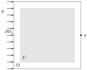
Figure 1: Setting of numerical experiments: Domain $\Omega$, area of interest $U$, incident light source $S(x)$ on the left, and detector point $\eta$ on the right.

4.1.2 Incident light field.

Since in our model the incident light intensity $u$ is independent of the shape and location of the ultrasound waves in the tissue, $u$ only needs to be computed once. For this computation, a finite element approximation to $u$ is constructed on a regular rectangular grid using ${\mathbb{Q}}_{1}$ finite elements [15], solving equations (6)–(8). The left panel of Fig. 2 shows $u$ for the case of a constant absorption coefficient $\mu$.

4.1.3 Ultrasound field.

In our numerical examples, we use Gaussian-shaped synthetic ultrasound signals:

$$p(x)=C\exp\bigg{(}-\sum_{j=1}^{d}\frac{|x_{j}|^{2}}{\sigma_{j}^{2}}\bigg{)},$$ (16)

where $C$ is a normalization constant. By choosing different variances $\sigma_{j}^{2}$ we can model varying focusing properties of such pressure field.

To simulate scanning of the ultrasound focus, focusing points $\{{\mathbf{\xi}}^{i},\;i=1,\ldots,N\}$ are placed at the vertices of a square grid covering the area of interest, here chosen as the square $U=[0.5\rm{cm},4.5\rm{cm}]^{2}\subset\Omega$. For each $i$ we then construct a signal $p^{\xi_{i}}(x)$ focused at $\xi_{i}$ by setting

$$p^{\xi_{i}}(x):=p(x-\xi_{i}).$$

To simplify notation we set $v^{i}:=v^{\xi^{i}}$ and $p^{i}:=p^{\xi^{i}}$.

4.1.4 Modulated light field and measurements.

Given $u$ and $|p^{i}|^{2}$, we compute the intensity of the modulated light $v^{i}(x)$, using equations (12). The equations are again solved using ${\mathbb{Q}}_{1}$ finite elements. Two examples for $v^{i}$ are shown in Fig. 2 for two different focus positions. The modulated light intensities $v^{i}$ are then evaluated at the sensor location $\eta$ to yield the measurements $h(\xi_{i})=v^{i}(\eta)$.

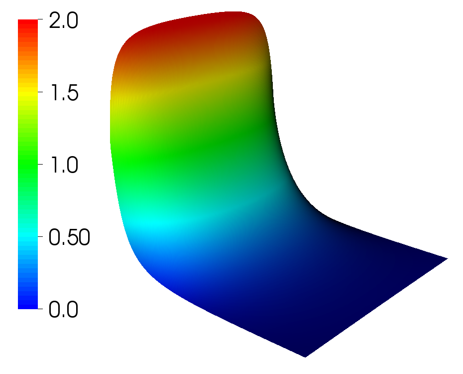
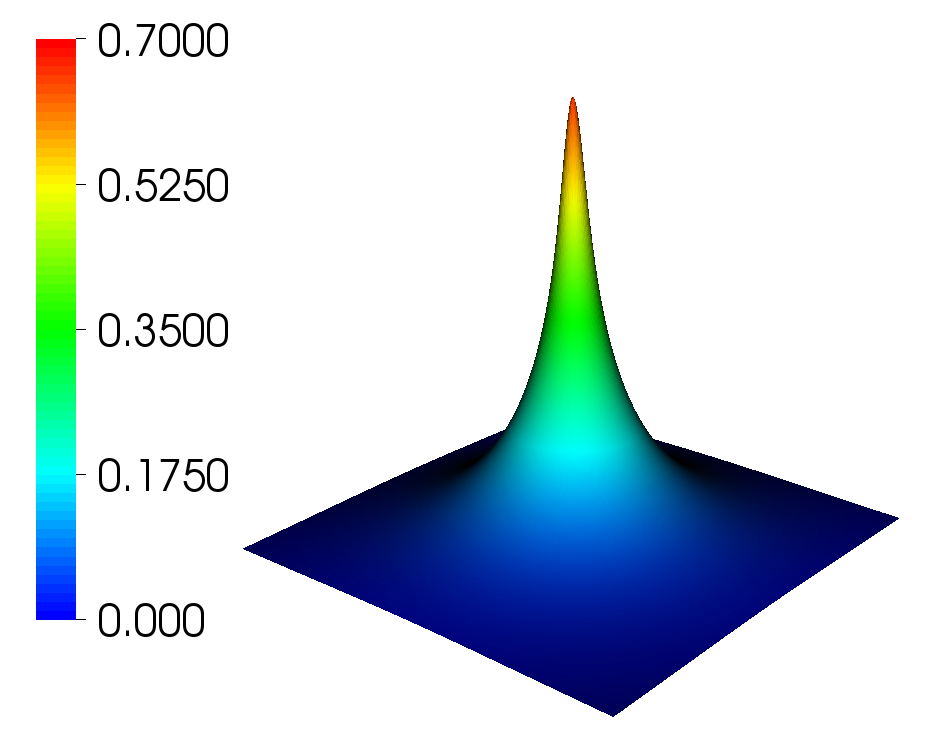
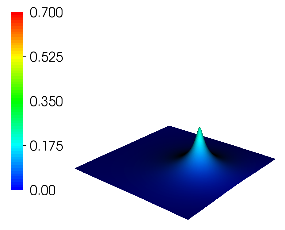
Figure 2: Left: Incident light intensity $u$ for constant absorption coefficient. Center and right: Modulated light intensity $v^{\xi}$ for two different focus points $\xi$. Note that $v$ depends on the focus position as well as the intensity of $u$ at the focus.

4.2 Green’s function and reconstruction

The reconstruction algorithm requires knowledge of the Green’s function $G$, which, given the absorption coefficient $\mu$ and resulting diffusion coefficient $D$, solves (13). Hence, we compute $G$ by solving another diffusion problem with homogeneous Robin boundary conditions and a suitable approximation to the delta function on the right hand side. As before, this is done using a finite element scheme, where we choose a different, coarser mesh than in forward problem calculations to avoid committing inverse crimes.

An obvious problem in the reconstruction formula (14) is that it involves derivatives of the measurement data $h(\xi)$, which causes instabilities in the presence of noise. Possible regularizations for this problem are well-studied (e.g. [6]), and the stability analysis in Section 5 suggests that this is the only source of instability in the reconstruction process. Hence, we opt not to add extra regularization and compute the derivatives by a simple central finite differencing scheme. Without adding noise to the measurements, it turned out that in all of our computational experiments, the regularization stemming from discretization on a fixed grid was sufficient for convergence of the iterative scheme based on (14).

4.3 Numerical phantoms

To test our algorithms, we use three test cases in which the true absorption coefficients have the following form:

• A disk-shaped inclusion $K\subset\Omega$ with midpoint $(2.5\rm{cm},2.5\rm{cm})$ and radius $0.5\rm{cm}$. The absorption coefficient is assumed to be equal to $\bar{\mu}$ outside the inclusion and slightly higher inside:

  $$\mu^{\ast}(x)=\left\{\begin{array}[2]{l@{\;}l}\bar{\mu}&,\quad x\in\Omega\setminus K\\ 1.2\,\bar{\mu}&,\quad x\in K.\end{array}\right.$$

• For the same inclusion $K$, a much higher absorption coefficient contrast

  $$\mu^{\ast}(x)=\left\{\begin{array}[2]{l@{\;}l}\bar{\mu}&,\quad x\in\Omega\setminus K\\ 10\,\bar{\mu}&,\quad x\in K.\end{array}\right.$$

• A more complicated coefficient with multiple inclusions of different magnitude between $1.2\,\bar{\mu}$ and $2.0\,\bar{\mu}$. Their exact shape is shown in Fig. 3. This case tests the ability of our algorithms to resolve several nearby objects.

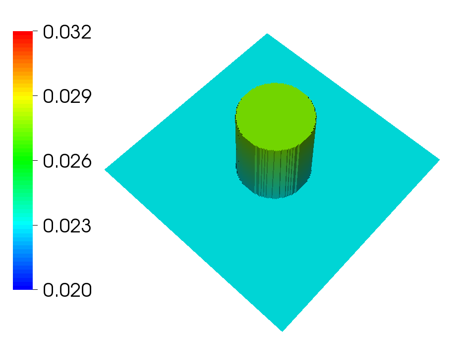
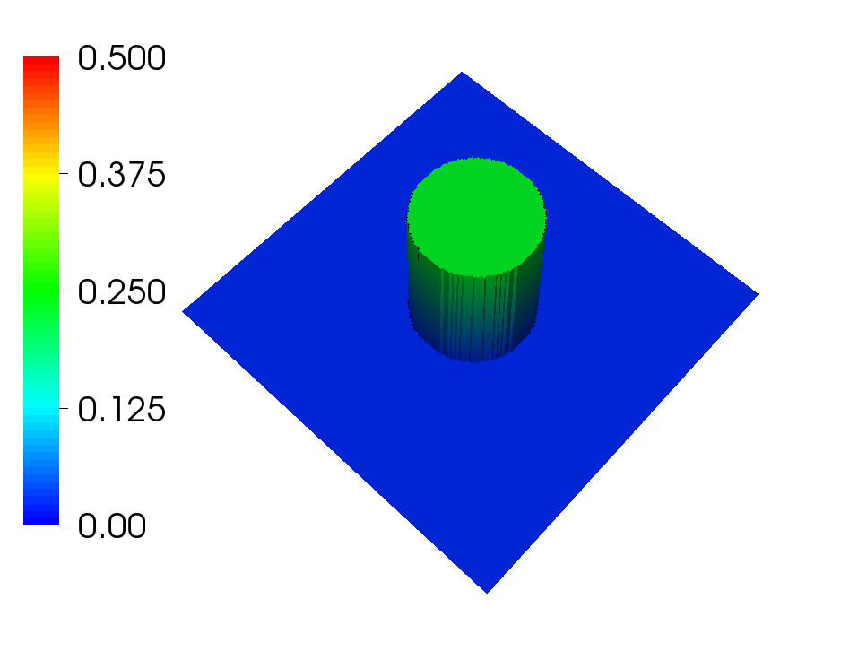
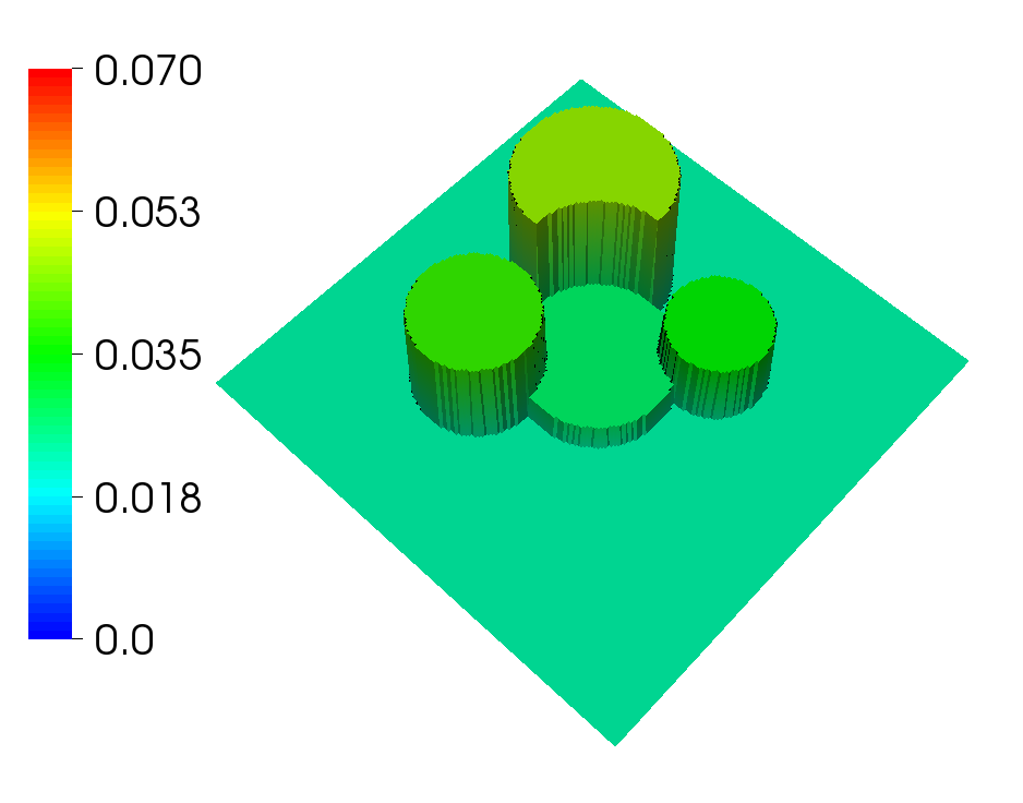
Figure 3: Test cases for absorption coefficient $\mu^{\ast}$.

For actual numerical values, we used $\bar{\mu}=0.023\rm{cm^{-1}}$, $\mu_{s}^{\prime}=10.74\rm{cm^{-1}}$ and $\gamma=0.431\rm{cm^{-1}}$ in our computations. These values represent typical optical properties of soft tissue [16].

4.4 Reconstruction results

For the results shown in this section, measurements were produced using the ultrasound signal arising from setting variances $\sigma_{1}=\sigma_{2}=0.1\rm{cm}$ in the Gaussian (16), resulting in sharp focusing in each direction (see the center panel of Fig. 5 below). Fig. 4 shows reconstructions of the three different absorption coefficients for scanning the ultrasound focus $\xi^{i}$ on a $100\!\times\!100$ mesh of points inside the area of interest $U$.

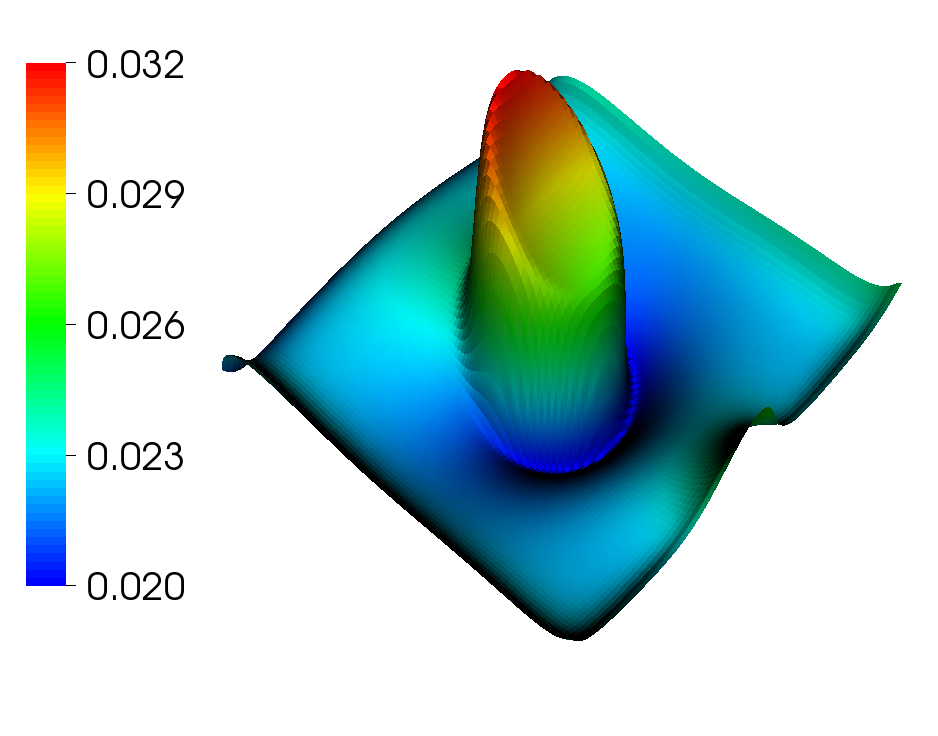
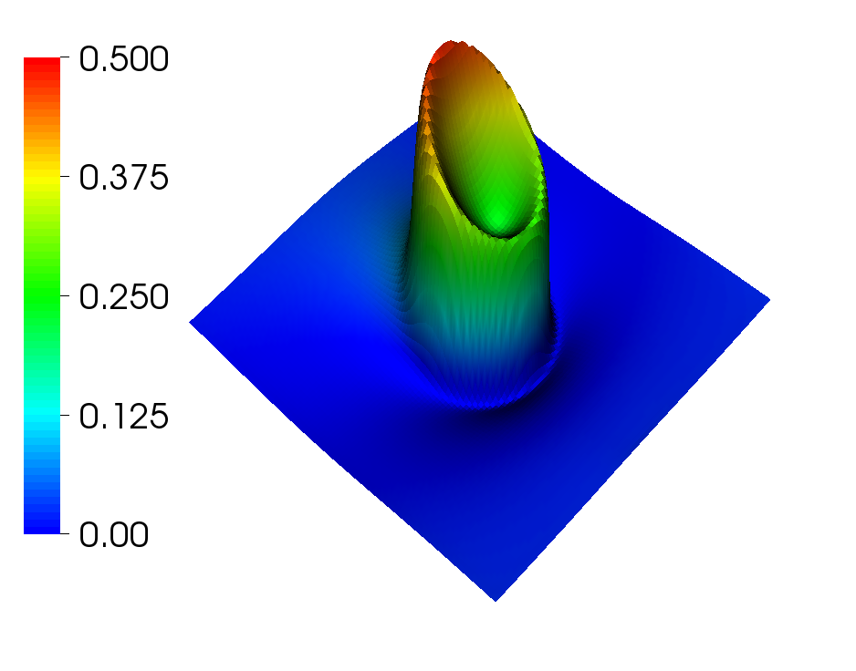
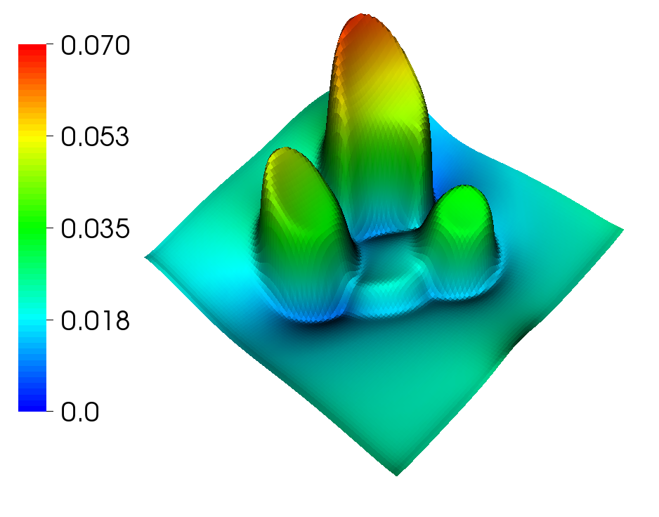
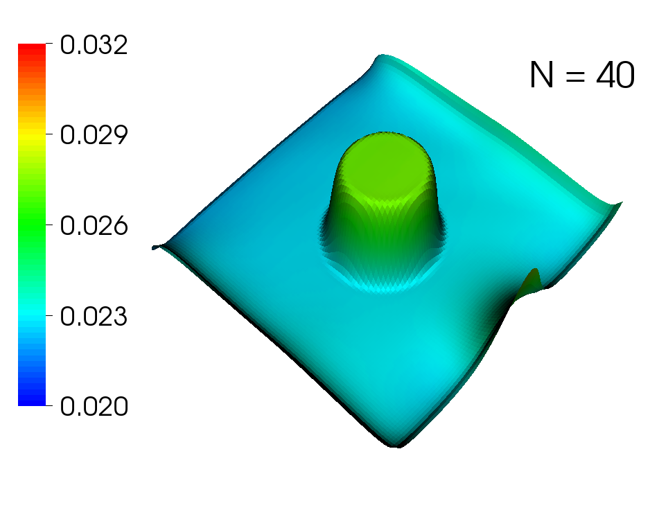
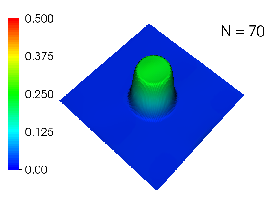
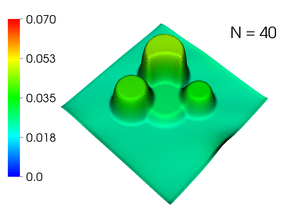
Figure 4: Reconstruction results for the three coefficient cases: after the first step of the algorithm (top) and after $N=40,70$ and $40$ iterations, respectively (bottom).

The principal observation from these results is that under the main assumptions of the model, i.e. turbid medium (and thus $\mu\ll\mu^{\prime}_{s}$), virtual light source, and strong focusing, our reconstruction scheme has four desirable properties:

• It converges, even for the second case where (i) we start far away from the exact coefficient and (ii) the exact coefficient has a large dynamic range.

• It is stable, i.e. the errors introduced through discretization of the equations, finite differencing of data, and using different meshes for reconstruction and generation of synthetic data do not lead to inaccurate reconstructions.

• It can recover sharp interfaces without excessive blurring.

• It can recover quantitatively correct values of absorption.

These are significant advantages compared to many other optical tomographic methodologies.

5 Stability of the linearized problem

The quality of reconstructions shown above, especially the recovery of sharp singularities, is at first surprising, given that the standard OT problem is strongly ill-posed. In this section, we will make a first step towards understanding the stability of the UOT procedure.

Note that even though equations (12) defining $u$ and $v$ are linear, the relation between the absorption coefficient $\mu$ and the measurements $h$ is nonlinear. In this section, we consider a (formal) linearization of the system (12) that will allow us to gain some insight into the local properties of the inverse problem.

Let $\Omega\subset{\mathbb{R}}^{d}$ with $d=2$ or $d=3$ be an open bounded domain with $C^{2}$-boundary. We use a formal linearization, assuming that $\mu$ is a small perturbation of a known absorption $\mu_{0}>0,\mu_{0}\in C^{0,1}(\overline{\Omega})$, and then applying the formal asymptotic expansions

$$\mu(x) \;=\; \mu_{0}(x)+{\varepsilon}\mu_{1}(x)+o({\varepsilon}),$$

$$u(x) \;=\; u_{0}(x)+{\varepsilon}u_{1}(x)+o({\varepsilon}),$$

$$v^{\xi}(x) \;=\; v_{0}^{\xi}(x)+{\varepsilon}v_{1}^{\xi}(x)+o({\varepsilon}),$$

where ${\varepsilon}\rightarrow 0$. Our goal is to relate the first order perturbations of the absorption coefficient $\mu_{1}$ and the measurements $h_{1}(\xi):=v_{1}^{\xi}(\eta)$, where $\eta\in\partial\Omega$ is the location of the detector.

Let us again assume perfectly focused ultrasound, i.e. $|p^{\xi}(x)|^{2}=\delta(x-\xi)$. By inserting the above expansions into equations (12) and sorting terms according to powers of ${\varepsilon}$, we then get the zeroth order perturbation system

$$-\nabla\cdot D\nabla u_{0}(x)+\mu_{0}(x)u_{0}(x) = 0,$$ (17)

$$-\nabla\cdot D\nabla v_{0}^{\xi}(x)+\mu_{0}(x)v_{0}^{\xi}(x) = \alpha\delta(x-\xi)u_{0}(x),$$ (18)

and the first order perturbation system

$$-\nabla\cdot D\nabla u_{1}(x)+\mu_{0}(x)u_{1}(x) = -\mu_{1}(x)u_{0}(x),$$ (19)

$$-\nabla\cdot D\nabla v_{1}^{\xi}(x)+\mu_{0}(x)v_{1}^{\xi}(x) = \alpha\delta(x-\xi)u_{1}(x)-\mu_{1}(x)v_{0}^{\xi}(x)$$ (20)

for all $x\in\Omega$, complemented by inhomogeneous Robin boundary conditions as in (8) for $u_{0}$ and homogeneous Robin boundary conditions for $v_{0}^{\xi}$, $u_{1}$ and $v_{1}^{\xi}$. Here we neglected the (weak) dependence of $D$ on $\mu$ and instead set $D\equiv\textrm{const}>0$ for the rest of this section.

Equations (17)–(18) imply that $u_{0}$ and $v_{0}^{\xi}$ are solutions to the forward model for absorption coefficient $\mu_{0}$. The standard elliptic regularity theorems (e.g., [17]) imply $u_{0}\in H^{3}(\Omega)$, and by the Sobolev embedding theorem $u_{0}\in C^{1}(\overline{\Omega})$ [18].

Let us assume that the absorption coefficient is known near the boundary, so that it suffices to consider perturbations $\mu_{1}$ supported in an open set $U$ with $C^{2}$-boundary such that $\overline{U}\subset\Omega$. We assume the data $h_{1}(\xi)$ to be given for all $\xi\in U$. In what follows, we derive an explicit formula for the dependence of $\mu_{1}$ on $h_{1}$ and then study properties of the corresponding linear operator.

Let us denote by $G_{0}(x,y)$ the Green’s function as defined in (13) corresponding to the background absorption coefficient $\mu_{0}$. Equation (18) implies that for all $x\in\Omega$ and $\xi\in U$,

$$v_{0}^{\xi}(x)\; = \;\int_{\Omega}\alpha G_{0}(x,z)\delta(z-\xi)u_{0}(z)\;dz$$

$$= \;\alpha G_{0}(x,\xi)u_{0}(\xi).$$

From (20) we can now deduce that

$$v_{1}^{\xi}(x)\; = \;\int_{\Omega}G_{0}(x,z)\left[\alpha\delta(z-\xi)u_{1}(z)-\mu_{1}(z)v_{0}^{\xi}(z)\right]\,dz$$

$$= \;\alpha G_{0}(x,\xi)u_{1}(\xi)-\alpha u_{0}(\xi)\int_{\Omega}G_{0}(x,z)G_{0}(z,\xi)\mu_{1}(z)\;dz.$$

Evaluating at $x=\eta$ and solving for $u_{1}$ yields

$$u_{1}(\xi)\;=\;\frac{h_{1}(\xi)}{\alpha G_{0}(\eta,\xi)}+\frac{u_{0}(\xi)}{G_{0}(\eta,\xi)}\int_{\Omega}G_{0}(\eta,z)G_{0}(z,\xi)\mu_{1}(z)\;dz.$$

We now use this expression to eliminate $u_{1}$ from (19). Noting that the differential operators now act on $\xi$ and that

$$\left[-\nabla_{\xi}\cdot D\nabla_{\xi}+\mu_{0}(\xi)\right]G_{0}(x,\xi)\;=\;\delta(x-\xi),$$

we get

$$0 =u_{0}(\xi)\mu_{1}(\xi)+\left[-\nabla_{\xi}\cdot D\nabla_{\xi}+\mu_{0}(\xi)\right]\left(\frac{h_{1}(\xi)}{\alpha G_{0}(\eta,\xi)}\right)$$

$$\qquad+\left[-\nabla_{\xi}\cdot D\nabla_{\xi}+\mu_{0}(\xi)\right]\left(\frac{u_{0}(\xi)}{G_{0}(\eta,\xi)}\int_{\Omega}G_{0}(\eta,z)G_{0}(z,\xi)\mu_{1}(z)\;dz\right)$$

$$=u_{0}(\xi)\mu_{1}(\xi)+\left[-\nabla_{\xi}\cdot D\nabla_{\xi}+\mu_{0}(\xi)\right]\left(\frac{h_{1}(\xi)}{\alpha G_{0}(\eta,\xi)}\right)$$

$$\qquad+\left(\left[-\nabla_{\xi}\cdot D\nabla_{\xi}\right]\left[\frac{u_{0}(\xi)}{G_{0}(\eta,\xi)}\right]\right)\int_{\Omega}G_{0}(\eta,z)G_{0}(z,\xi)\mu_{1}(z)\;dz$$

$$\qquad-2D\left[\nabla_{\xi}\left(\frac{u_{0}(\xi)}{G_{0}(\eta,\xi)}\right)\right]\cdot\left[\nabla_{\xi}\int_{\Omega}G_{0}(\eta,z)G_{0}(z,\xi)\mu_{1}(z)\;dz\right]$$

$$\qquad+\frac{u_{0}(\xi)}{G_{0}(\eta,\xi)}G_{0}(\eta,\xi)\mu_{1}(\xi).$$

We will frequently view $G_{0}(\eta,y)$ as a function of $y$ in the following and hence introduce the notation

$$G_{0}^{\eta}(y):=G_{0}(\eta,y)\quad\textrm{for }y\in\overline{U}.$$

Note that since $\eta\in\partial\Omega$, $G_{0}^{\eta}$ has no singularities on $\overline{U}$ and hence is a regular solution to (17) there. The elliptic regularity and Sobolev embeddings imply $G_{0}^{\eta}\in C^{1}(\overline{U})$.

Let us define the following operators acting on functions $g$ defined on $U$:

$$K_{1}g(\xi) :=-\frac{1}{2u_{0}(\xi)}\left(\left[-\nabla_{\xi}\cdot D\nabla_{\xi}\right]\left[\frac{u_{0}(\xi)}{G_{0}^{\eta}(\xi)}\right]\right)\int_{U}G_{0}^{\eta}(z)G_{0}(z,\xi)g(z)\;dz,$$ (21)

$$K_{2}g(\xi) :=\frac{D}{u_{0}(\xi)}\left[\nabla_{\xi}\left(\frac{u_{0}(\xi)}{G_{0}^{\eta}(\xi)}\right)\right]\cdot\left[\nabla_{\xi}\int_{U}G_{0}^{\eta}(z)G_{0}(z,\xi)g(z)\;dz\right],$$ (22)

and

$$F:=1-K_{1}-K_{2}.$$

In terms of these operators, our considerations above imply that $\mu_{1}$ is a solution to the following linear equation:

$$F\mu_{1}(\xi)\;=\;-\frac{1}{2u_{0}(\xi)}\left[-\nabla_{\xi}\cdot D\nabla_{\xi}+\mu_{0}(\xi)\right]\left(\frac{h_{1}(\xi)}{\alpha G_{0}^{\eta}(\xi)}\right)$$ (23)

In order for the above expressions to be well-defined, we have to make sure that $u_{0}$ and $G_{0}^{\eta}$ are bounded away from zero on $\overline{U}$. The following lemma follows immediately from the Hopf Lemma (e.g., [19, 20]):

Lemma 1

There is a constant $c>0$ such that $u_{0}\geq c$ and $G_{0}^{\eta}\geq c$ on $\overline{U}$.

Next we consider the properties of the integral term involved in $K_{1}$ and $K_{2}$. The important observation here is the following:

Lemma 2

The mapping

$$g\mapsto\int_{U}G_{0}(z,\cdot)G_{0}^{\eta}(z)g(z)\,dz$$ (24)

is a bounded linear operator from $L^{2}(U)$ to $H^{2}(U)$.

Proof: Let us assume that $g\in L^{2}(U)$. Since $G_{0}^{\eta}\in C(\overline{U})$, multiplication by $G_{0}^{\eta}$ is a bounded linear operator on $L^{2}(U)$. The following integration against $G_{0}(z,\cdot)$ results in the solution to the diffusion equation with homogeneous Robin boundary condition and right hand side $G_{0}^{\eta}g\in L^{2}(U)$. Elliptic regularity theory (e.g., [17, 18]) implies that this is a continuous operator from $L^{2}(U)$ into $H^{2}(U)$. $\scriptstyle{\Box}$

Because of the compact embedding of $H^{2}(U)$ in $L^{2}(U)$, the operator defined by (24), viewed as a mapping from $L^{2}(U)$ to $L^{2}(U)$, is compact. In (21), this operator is multiplied by the factor

$$-\frac{1}{2u_{0}(\xi)}\left(\left[-\nabla_{\xi}\cdot D\nabla_{\xi}\right]\left[\frac{u_{0}(\xi)}{G_{0}^{\eta}(\xi)}\right]\right).$$ (25)

The functions $u_{0},\nabla u_{0},G_{0}^{\eta}$ and $\nabla G_{0}^{\eta}$ are all bounded on $\overline{U}$ because $u_{0},G_{0}^{\eta}\in C^{1}(\overline{U})$. Since $u_{0}$ and $G_{0}^{\eta}$ satisfy (17), the terms $\nabla\cdot D\nabla u_{0}$ and $\nabla\cdot D\nabla G_{0}^{\eta}$ are bounded on $\overline{U}$ as well, and $u_{0}^{-1}$ and $(G_{0}^{\eta})^{-1}$ are bounded due to Lemma 1. Consequently, multiplication by (25) represents a bounded linear operation on $L^{2}(U)$, and so $K_{1}$ is a compact operator in $L^{2}(U)$. Similarly, $K_{2}$ is a compact operator in $L^{2}(U)$. This leads us to the main result of this section:

Theorem 3

$F:L^{2}(U)\to L^{2}(U)$ is a Fredholm operator of index zero.

Thus, the kernel ${\cal N}(F)$ of $F$ has finite dimension and the range ${\cal R}(F)$ is closed and of finite codimension, equal to the dimension of the kernel. This immediately implies the following result:

Corollary 4

$F$ as an operator from the quotient space $L^{2}(U)/{\cal N}(F)$ to ${\cal R}(F)$ has bounded inverse, and the following norm equivalence holds:

$$c_{1}\|Ff\|_{L^{2}(U)}\;\leq\;\|f\|_{L^{2}(U)/{\cal N}(F)}\;\leq\;c_{2}\|Ff\|_{L^{2}(U)}.$$ (26)

The $L^{2}$-norm of the right hand side expression in (23) can be estimated in terms of the $H^{2}$-norm of the measured perturbation $h_{1}$, so that we obtain the following stability result:

Theorem 5

Under the stated assumptions, there is a constant $C>0$ such that the following relation holds:

$$\|\mu_{1}\|_{L^{2}(U)/{\cal N}(F)}\;\leq\;C\|h_{1}\|_{H^{2}(U)}.$$ (27)

We conjecture that the kernel ${\cal N}(F)$ is in fact trivial, and thus the operator $F$ is invertible. This would imply that $\mu_{1}$ is uniquely determined by the measured perturbation $h_{1}$, and allow us to replace the quotient space norms in (26) and (27) with the regular $L^{2}$ norms. However, we have not been able to prove this result yet.

Smoother norm coercive estimates for the absorption can be obtained if more is assumed about the unperturbed absorption $\mu_{0}$ and the domain. For instance, if $\mu_{0}\in C^{\infty}(\Omega)$, $S\in C^{\infty}(\partial\Omega)$, and $\Omega$ has smooth boundary, the operators $K_{1}$ and $K_{2}$ defined in (21)–(22), are of order $-2$ and $-1$, respectively, in the Sobolev scale:

$$K_{1}\; : \;H^{s}(U)\to H^{s+2}(U),$$

$$K_{2}\; : \;H^{s}(U)\to H^{s+1}(U).$$

This and the Sobolev embedding theorem [21] imply that for any $s\geq 0$, $F$ is Fredholm as an operator

$$F\;:\;H^{s}(U)\to H^{s}(U).$$

This, in turn, leads to the estimate

$$\|f\|_{H^{s}(U)}\;\leq\;c\left(\|f\|_{L^{2}(U)}+\|Ff\|_{H^{s}(U)}\right)$$ (28)

for all $f\in H^{s}(U)$. Thus, we have the following result:

Theorem 6

Under the stated assumptions, for any $s>0$ there is a constant $C$ such that

$$\|\mu_{1}\|_{H^{s}(U)}\;\leq\;C\left(\|\mu_{1}\|_{L^{2}(U)}+\|h_{1}\|_{H^{s+2}(U)}\right).$$

Clearly, if only a specific value of $s$ is of interest, the smoothness assumptions on $\mu_{0},S$ and $\partial\Omega$ can be relaxed appropriately.

6 Conclusion and outlook

In this paper, we have introduced a partial differential equation model of ultrasound modulated optical tomography to derive a simple reconstruction scheme for recovering the spatially varying absorption coefficient from boundary measurements. While we could demonstrate stable, sharp and quantitatively accurate reconstructions, some of the assumptions made here need to or can be improved upon for practical applications. In particular, these are:

Detector locations

In the discussion of stability above, as well as in our numerical reconstructions, we have chosen a single detector point $\eta$. However, using detectors distributed over a part $\Gamma$ of the boundary $\partial\Omega$ should help to suppress the effect of noise in the measured data.

Ultrasound signal with elongated focus

In practice, perfect focusing of ultrasound waves is not a realistic assumption [22]. How well an ultrasound signal can be focused depends, in particular, on the geometry and bandwidth of the transducer. For example, it is known from experimental measurements (e.g., [23]) that focused ultrasound signals have an intensity profile similar to the one shown in Fig. 5 (left). This signal has significantly sharper focus in the direction transverse to the transducer lens, while the well-focused Gaussian signal used in our results does not reflect this behavior.

Figure 5: Left: Simulated ultrasound pressure field $|p|^{2}$ with transducer at the bottom. Middle: Gaussian ultrasound signal $|p|^{2}$ with $\sigma_{1}=\sigma_{2}=0.1$. Right: Gaussian signal with $\sigma_{1}=0.1$, $\sigma_{2}=0.3$.

To illustrate the effect of relaxing the assumption of perfect focus, we computed reconstructions for the case where the ultrasound intensity is a Gaussian signal with sharp focus in $x$-direction and elongated focus in $y$-direction (Fig. 5, right). As in the previous section, the ultrasound focus $\xi^{i}$ is scanned on a $100\!\times\!100$ mesh to produce synthetic measurements. At the same time, the reconstruction algorithm is left unchanged, i.e. still assumes perfect focus.

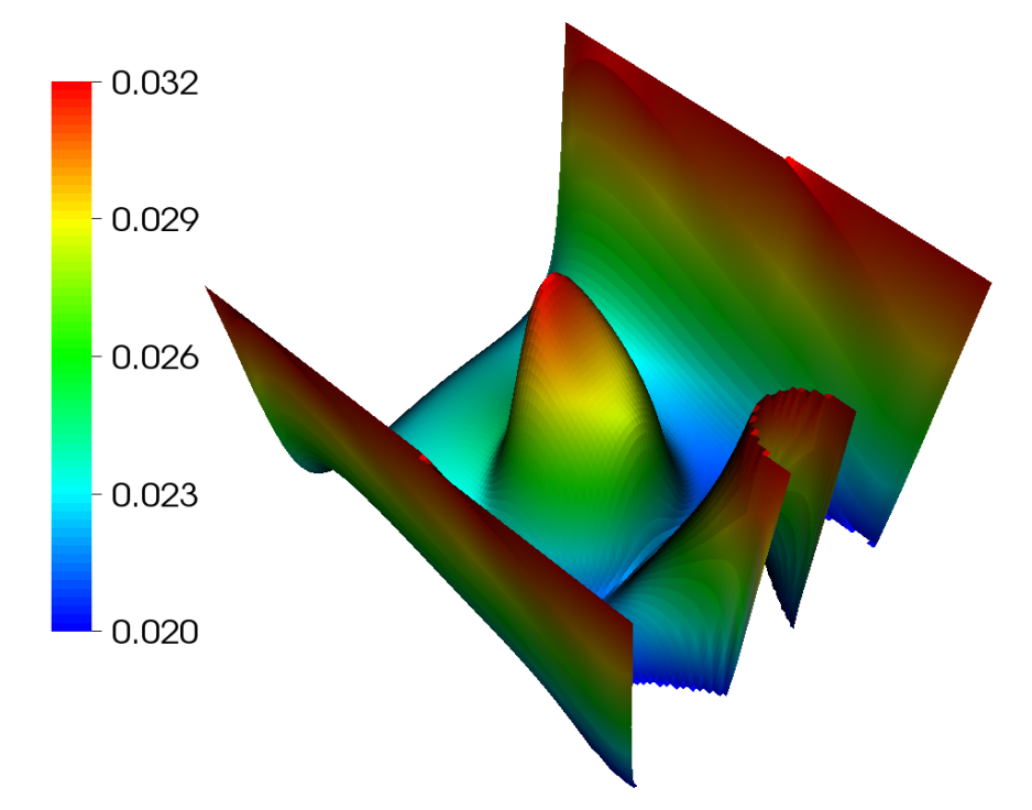
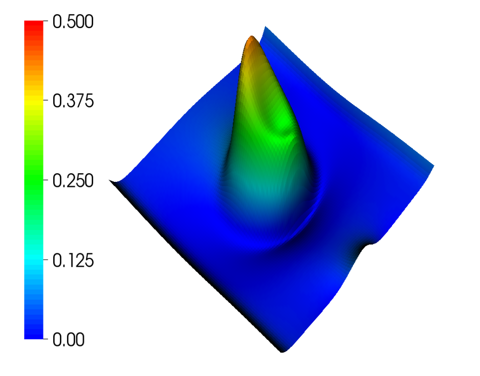
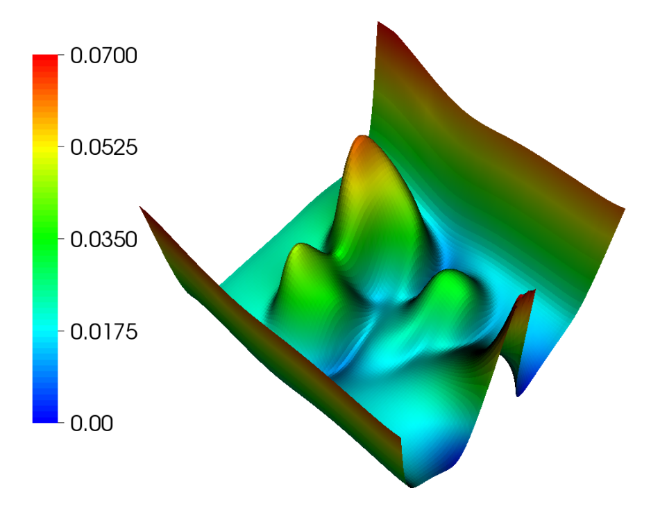
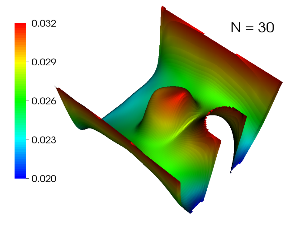
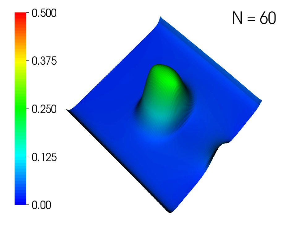
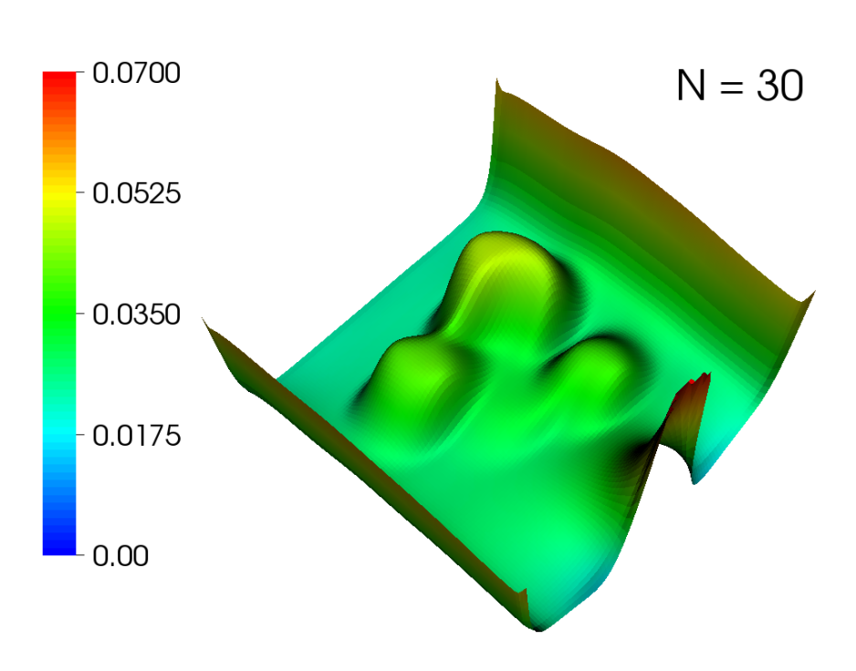
Figure 6: Reconstruction results for ultrasound signal with elongated focus: after the first step of the algorithm (top) and after $N$ iterations (bottom).

Reconstruction results are shown in Fig. 6. The deterioration of the reconstruction – in particular in the direction of the ultrasound beam – is obvious. The results also contain artifacts at the vertical boundaries and close to the detector location. A more sophisticated reconstruction scheme might be needed to treat the non-perfect focusing in these calculations.

Synthetic focusing

Instead of attempting to perfectly focus the ultrasound waves in space, synthetic focusing allows the use of non-localized ultrasound fields and reconstructs the signal by superposition. This approach was suggested in [24]: It combines various basis sets of non-focused ultrasound waves (e.g., spherical or monochromatic planar ones), with a post-processing step that synthesizes the would-be response to a focused illumination. In particular, in the case of spherical waves, the post-processing (synthetic focusing procedure) is essentially equivalent to thermoacoustic tomography inversion (see [25]). We plan to investigate the applicability of this approach to UOT in the future.

Uniqueness of reconstruction

Proving uniqueness of reconstruction, both in the non-linear and linearized versions, still remains a challenge. In particular, we conjecture that the operator $F$ in (23) is in fact invertible, and thus there is uniqueness of solution of the linearized problem, which would replace the quotient space norms in (26) and (27) with the regular $L^{2}$ norms. At the same time, a complete characterization of the kernel of the operator $F$ is non-trivial and left for future work.

Summary

Despite these opportunities for future work, in this paper, a diffusion based model is provided for the ultrasound modulated optical tomography procedure using well focused ultrasound waves. An iterative algorithm is suggested to recover absorption from measurements of the amplitude of ultrasound modulation. The provided numerical results show feasibility of the algorithm and possibility of good reconstructions, both with regard to locating sharp interfaces, as well as recovering correct numerical values of the absorption coefficient. Such stability and resolution are impossible to achieve in standard optical tomography. The stability of reconstructions is explained by the stability estimates derived in Theorems 5 and 6 for a linearized model.

References

- Wang and Wu [2007] L. V. Wang, S.-I. Wu, Biomedical Optics. Principles and Imaging, Wiley-Interscience, Hoboken, NJ, 2007.
- Leutz and Maret [1995] W. Leutz, G. Maret, Ultrasonic modulation of multiply scattered light, Physica B 204 (1995) 14–19.
- Sevick-Muraca et al. [2003] E. M. Sevick-Muraca, E. Kuwana, A. Godavarty, J. P. Houston, A. B. Thompson, R. Roy, Near infrared fluorescence imaging and spectroscopy in random media and tissues, Biomedical Photonics Handbook, CRC Press.
- Kempe et al. [1997] M. Kempe, M. Larionov, D. Zaslavsky, A. Z. Genack, Acousto-optic tomography with multiply scattered light, J. Opt. Soc. Am. A 14 (1997) 1151–1158.
- Wang [2001] L. V. Wang, Mechanisms of ultrasonic modulation of multiply scattered coherent light: an analytic model, Phys. Rev. Lett. 87 (2001) 43903/1–4.
- Nam [2002] H. Nam, Ultrasound modulated optical tomography, Ph.D. thesis, Texas A&M University, 2002.
- Wang [2004] L. V. Wang, Ultrasound-mediated biophotonic imaging: A review of acousto-optical tomography and photo-acoustic tomography, Disease Markers 19 (2003/2004) 123–138.
- Chandrasekhar [1960] S. Chandrasekhar, Radiative Transfer, Dover, 1960.
- Godavarty et al. [2002] A. Godavarty, D. J. Hawrysz, R. Roy, E. M. Sevick-Muraca, The influence of the index-mismatch at the boundaries measured in fluorescence-enhanced frequency-domain photon migration imaging, Optics Express 10 (2002) 653–662.
- Sato and Ueno [1965] K. Sato, T. Ueno, Multi-dimensional diffusion and the Markov process on the boundary, J. Math. Kyoto Univ. 4 (1964/1965) 529–605.
- Gallavotti and McKean [1972] G. Gallavotti, H. P. McKean, Boundary conditions for the heat equation in a several-dimensional region, Nagoya Math. J. 47 (1972) 1–14.
- Del Grosso and Campanino [1976] G. Del Grosso, M. Campanino, A construction of the stochastic process associated to heat diffusion in a polygonal region, Boll. Un. Mat. Ital. B (5) 13 (1976) 876–895.
- Bangerth et al. [2007] W. Bangerth, R. Hartmann, G. Kanschat, deal.II – a general purpose object oriented finite element library, ACM Trans. Math. Softw. 33 (2007) 24/1–24/27.
- Bangerth et al. [2009] W. Bangerth, R. Hartmann, G. Kanschat, deal.II Differential Equations Analysis Library, Technical Reference, 2009. http://www.dealii.org/.
- Brenner and Scott [2002] S. C. Brenner, R. L. Scott, The Mathematical Theory of Finite Elements, Springer, Berlin-Heidelberg-New York, 2nd edition, 2002.
- Mobley and Vo-Dinh [2003] J. Mobley, T. Vo-Dinh, Optical Properties of Tissue, Biomedical Photonics Handbook, CRC Press.
- Gilbarg and Trudinger [2001] D. Gilbarg, N. S. Trudinger, Elliptic Partial Differential Equations of Second Order, volume 224 of Grundlehren der mathematischen Wissenschaften, Springer, 2001.
- Evans [1998] L. C. Evans, Partial differential equations, American Mathematical Society, Providence, RI, 1998.
- Li and Nirenberg [2007] Y. Y. Li, L. Nirenberg, On the Hopf lemma, preprint, arXiv:0709.3531v1 (2007).
- Protter and Weinberger [1984] M. H. Protter, H. F. Weinberger, Maximum principles in differential equations, Springer- Verlag, New York, 1984.
- Adams [1975] R. A. Adams, Sobolev Spaces, Pure and Applied Mathematics, Academic Press, 1975.
- Hernandez-Figueroa et al. [2008] H. E. Hernandez-Figueroa, M. Zamboni-Rached, E. R. (Editors), Localized Waves, IEEE Press, J. Wiley & Sons, Inc., Hoboken, NJ, 2008.
- Lévêque-Fort [2001] S. Lévêque-Fort, Three-dimensional acousto-optic imaging in biological tissues with parallel signal processing, Applied Optics 40 (2001) 1029–1036.
- Kuchment and Kunyansky [2010] P. Kuchment, L. Kunyansky, Synthetic focusing in ultrasound modulated tomography, Inverse Problems and Imaging, to appear (2010).
- Kuchment and Kunyansky [2008] P. Kuchment, L. Kunyansky, Mathematics of thermoacoustic tomography, European J. Appl. Math. 19 (2008) 191–224.