DILAND: An Algorithm for Distributed Sensor Localization with Noisy Distance Measurements

Abstract

In this correspondence, we present an algorithm for distributed sensor localization with noisy distance measurements (DILAND) that extends and makes the DLRE more robust. DLRE is a distributed sensor localization algorithm in $\mathbb{R}^{m}~{}(m\geq 1)$ introduced in [1]. DILAND operates when (i) the communication among the sensors is noisy; (ii) the communication links in the network may fail with a non-zero probability; and (iii) the measurements performed to compute distances among the sensors are corrupted with noise. The sensors (which do not know their locations) lie in the convex hull of at least $m+1$ anchors (nodes that know their own locations.) Under minimal assumptions on the connectivity and triangulation of each sensor in the network, this correspondence shows that, under the broad random phenomena described above, DILAND converges almost surely (a.s.) to the exact sensor locations.

Keywords: Distributed iterative sensor localization; sensor networks; Cayley-Menger determinant; barycentric coordinates; absorbing Markov chain; stochastic approximation; anchor.

I Introduction

Localization is an important problem in sensor networks, not only on its own right, but often as the first step toward solving more complicated and diverse network tasks, which may include environment monitoring, intrusion detection, and routing in geographically distributed communication networks. The problem we consider is when a large number of sensors do not know their locations, only a very few of them know their own. In [1], we presented a distributed sensor localization (DILOC) algorithm in $\mathbb{R}^{m}~{}(m\geq 1)$, when we can divide the $N$ nodes in the sensor network into these two sets: the set $\kappa$ of $n$ anchors where $n\geq m+1$ and the set $\Omega$ of $M$ sensors, with typically $N\gg n$. The $n$ anchors are the nodes that know their exact locations, whereas the $M$ sensors are the nodes that do not know their locations. We assume that the sensors lie in the convex hull of the anchors, i.e., $\mathcal{C}(\Omega)\subset\mathcal{C}(\kappa)$, where $\mathcal{C}(\cdot)$ denotes the convex hull. To each sensor $l$ in the network, we associate a triangulation set, $\Theta_{l}$, which is a set of $m+1$ neighboring nodes such that sensor $l$ lies in their convex hull, i.e., $l\in\mathcal{C}(\Theta_{l})$. In DILOC, each sensor, $l$, updates its location estimate as a linear convex combination of the estimates of the nodes in its triangulation set, $\Theta_{l}$, where the coefficients of the linear combination are the barycentric coordinates. Under minimal assumptions on network connectivity, and that the sensor $l$ knows the precise distances in the set

$$\mathcal{D}_{l}\triangleq\{l\}\cup\Theta_{l},$$ (1)

reference [1] shows that DILOC converges to the exact sensor locations. An interesting contribution of DILOC is that it reduces the centralized nonlinear problem of localization to a linear distributed iterative algorithm under broad assumptions, which can be implemented through local inter-sensor communication in real-time.

Reference [1] extends DILOC and presents a distributed localization algorithm in random environments (DLRE). DLRE is a stochastic approximation version of DILOC where the DILOC iterations are weighted with a decreasing weight sequence that follows a persistence condition. DLRE operates under the following random phenomena: (B.1) the communication among the sensors and the nodes in their triangulation set is noisy, i.e., at the $t$-th iteration, sensor $l$ receives only corrupted versions, $y_{ln}^{j}(t)$, $1\leq j\leq m$, of the $m$ components of the neighboring node $n$’s state, i.e., $x_{n}^{j}(t)$, given by

$$y_{ln}^{j}(t)=x_{n}^{j}(t)+v_{ln}^{j}(t),\qquad n\in\Theta_{l},$$ (2)

where $\left\{v_{ln}^{j}(t)\right\}_{l,n,j,t}$ is a family of independent zero-mean random variables with finite second moments; (B.2) each inter-node communication link is modeled by a binary random variable, $e_{ln}(t),l\in\Omega,n\in\Theta_{l}$, which is $1$ (active link) with probability $q_{ln}$, and $0$ (link failure) with probability $1-q_{nl}$; and (B.3) the local barycentric coordinates, computed at iteration $t$ from the current noisy distance measurements, can be represented as a perturbation of the exact barycentric coordinates. Reference [1] shows that, under (B.1)–(B.3) and if the perturbation in (B.3) is unbiased, DLRE converges to the sensor exact locations; however, if the perturbation in (B.3) is biased, DLRE converges with a steady-state error (bias).

In this correspondence, we modify DLRE to present the algorithm DILAND (distributed sensor localization with noisy distance measurements) and show that it converges a.s. to the exact sensor locations under much broader distance measurement noise assumptions. In DILAND, we replace (B.3) above with the following weaker condition: $\overline{\mbox{{(B.3)}}}$ at every iteration $t$, we assume there exist computationally efficient estimates of the required inter-sensor distances based on all distance measurements till time $t$ such that these estimates are consistent, i.e., they converge a.s. to the exact distances as $t\rightarrow\infty$. The state update in DILAND uses these estimates to compute the local barycentric coordinates, whereas the update in DLRE uses only the current distance measurements. The consistency assumption on the estimates of the inter-sensor distances is quite weak and, as will be shown, is applicable under practical schemes of estimating inter-sensor distances through: (i) received signal strength (RSS) and (ii) time-of-arrival (TOA) (see [3].) We emphasize that DILAND does not require spatial or temporal distributional assumptions on either the communication or the distance measurement noises, except for finiteness of the second order moment, see (B.1).

Because of (B.3), DLRE [1] converges to the exact sensor locations with a steady state error when the resulting perturbation of the barycentric coordinates is biased. In contrast, under the new assumption $\overline{\mbox{\bf(B.3)}}$, DILAND converges to the exact sensor locations regardless of the bias introduced in the system matrix (at each iteration) due to noisy distance measurements. This new setup leads to a behavior and analysis for DILAND that is different from DLRE’s in [1]. This is because using distance estimates based on the entire past leads to an inherent strong statistical dependence in the iterative scheme. This dependence makes the analysis of DILAND different from standard stochastic approximation arguments, which were used in [1] to prove the convergence properties of DLRE. Furthermore (as we will show in Section III-C), if we do not have link failures and communication noise, the weight sequence, $\alpha(t)$, in DILAND does not require the square summability condition required by DLRE. Hence, DILAND can be designed to converge faster than DLRE by choosing the DILAND weight sequence to sum faster to infinity than the DLRE weight sequence.

We describe the rest of the paper. Section II briefly recapitulates our prior work on DILOC and DLRE. We then study the distance estimates and present the main result, DILAND, of this correspondence in Section III. Section IV presents simulations, and Section V concludes the paper.

II Prior Work

We briefly recapitulate the setting of the distributed localization problem, details and discussions are in [1].

II-A Distributed Localization Algorithm (DILOC)

Let the row vector $\mathbf{x}_{l}(t)\in\mathbb{R}^{1\times m},l\in\Omega$, be the $m$-dimensional state that represents the estimated coordinates of sensor $l$ at time $t$. Similarly, let the row vector $\mathbf{u}_{k}\in\mathbb{R}^{1\times m},~{}k\in\kappa,$ be the $m$-dimensional state of the location coordinates of anchor $k$. DILOC updates at time $t$ are the following:

$$\mathbf{u}_{k}(t+1) = \mathbf{u}_{k}(t),\qquad\qquad\qquad\qquad\qquad\qquad~{}~{}~{}k\in\kappa,$$ (3)

$$\mathbf{x}_{l}(t+1) = \sum_{n\in{\Omega\cap\Theta_{l}}}p_{ln}\mathbf{x}_{n}(t)+\sum_{k\in{\kappa\cap\Theta_{l}}}b_{lk}\mathbf{u}_{k},\qquad l\in\Omega.$$ (4)

The symbol $\Theta_{l}$ is the triangulation set of sensor $l$, and $p_{ln}$ and $b_{lk}$ are the sensor-sensor and the sensor-anchor barycentric coordinates, [4], respectively; these are computed using the inter-node distances in $\mathcal{D}_{l}$ and the Cayley-Menger determinants [5] (see [1].) Let the set of inter-sensor distances required to compute all the barycentric coordinates be ($\ast$ represents the exact value)

$$\mathbf{d}^{\ast}=\{d^{\ast}_{kn}~{}|~{}k,n\in\mathcal{D}_{l},l\in\Omega\}.$$ (5)

The barycentric coordinates lead to the system matrices $\mathbf{P}\left(\mathbf{d}^{\ast}\right)=\left\{p_{ln}\right\}$ and $\mathbf{B}\left(\mathbf{d}^{\ast}\right)=\left\{b_{lk}\right\}$ of DILOC (we use $\left(\mathbf{d}^{\ast}\right)$ to show an implicit dependence on the inter-sensor distances.) We define the matrix $\mathbf{X}(t)$ collecting the row vector states $\mathbf{x}_{l}(t)$ for all sensors $l$ and with column vectors $\mathbf{x}^{j}(t)$; similarly for $\mathbf{U}$.

$$M\times m:\>\mathbf{X}(t) = \left[\mathbf{x}_{1}(t)^{T},\ldots,\mathbf{x}_{M}(t)^{T}\right]^{T}=\left[\mathbf{x}^{1}(t)\cdots\mathbf{x}^{j}(t)\cdots\mathbf{x}^{m}(t)\right]$$ (6)

$$(m+1)\times m:\>\mathbf{U} = \left[\mathbf{u}_{1}^{T},\ldots,\mathbf{u}_{m+1}^{T}\right]^{T}=\left[\mathbf{u}^{1}(t)\cdots\mathbf{u}^{j}(t)\cdots\mathbf{u}^{m}(t)\right].$$ (7)

In (6) and (7), sub and superindices indicate row and column vectors of the corresponding matrices, i.e., $\mathbf{x}^{j}(t)$ is the column vector that collects component $j$ of the row vector state $\mathbf{x}_{l}(t)$ of all sensors $l$; similarly for $\mathbf{u}^{j}(t)$.

We recall from [1] the following assumptions.

Structural assumptions: (A1) There are at least $m+1$ anchors, i.e., $|\kappa|=n=m+1$, that do not lie on a hyperplane in $\mathbb{R}^{m}$; (A2) The $M$ sensors lie inside the convex hull of the anchors, i.e., $\mathcal{C}(\Omega)\subseteq\mathcal{C}(\kappa)$, where $\mathcal{C}(\cdot)$ denotes the convex hull; (A3) There exists a triangulation set, $\Theta_{l}\subset\Theta,~{}\forall~{}l\in\Omega$, with $|\Theta_{l}|=m+1$, such that $l\in\mathcal{C}(\Theta_{l})$; (A4) The sensor $l$ is assumed to have a communication link, $n\rightarrow l$, to each $n\in\Theta_{l}$ and the inter-node distances among all the sensors in the set $\mathcal{D}_{l}$ are known at sensor $l$; and (A5) Each anchor, $k\in\kappa$, has a communication link to at least one sensor in $\Omega$.

Theorem 1 (Theorem 1, [1])

Under (A1)-(A5), for DILOC (4), $\lim_{t\rightarrow\infty}\mathbf{X}(t+1)=(\mathbf{I-P}(\mathbf{d}^{\ast}))^{-1}\mathbf{B}(\mathbf{d}^{\ast})\mathbf{U}$, i.e., the states converge to the exact sensor locations.

II-B Distributed Localization in Random Environments (DLRE)

We start by contrasting assumptions (B.3) and $\overline{\mbox{\bf(B.3)}}$ (introduced in Section I).

(B.3) Small perturbation of system matrices: Recall from Section I that at each sensor $l$ the distances required to compute the barycentric coordinates are the inter-node distances in the set $\mathcal{D}_{l}$. In reality, the sensors do not know the precise distances, $d_{(\cdot)(\cdot)}^{\ast}$, but estimate the distances $\widehat{d}_{(\cdot)(\cdot)}(t)$, from RSS or TOA measurements at time $t$. When we have noisy distance measurements, we iterate with system matrices $\mathbf{P}(\widehat{\mathbf{d}}_{t})$ and $\mathbf{B}(\widehat{\mathbf{d}}_{t})$, not with $\mathbf{P}(\mathbf{d}^{\ast})$ and $\mathbf{B}(\mathbf{d}^{\ast})$, where $\widehat{\mathbf{d}}_{t}$ is the set like $\mathbf{d}^{\ast}$ in (5) that collects all required inter-node distance estimates $\widehat{d}_{kn}(t)$, $k,n\in\mathcal{D}_{l},l\in\Omega$. Assuming the distance measurements are statistically independent over time, $\mathbf{P}(\widehat{\mathbf{d}}_{t})$ and $\mathbf{B}(\widehat{\mathbf{d}}_{t})$ can be written as

$$\mathbf{P}\left(\widehat{\mathbf{d}}_{t}\right) =\mathbf{P}(\mathbf{d}^{\ast})+\mathbf{S}_{\mathbf{P}}+\widetilde{\mathbf{S}}_{\mathbf{P}}(t)\triangleq\{\widehat{p}_{ln}(t)\}, \mathbf{B}\left(\widehat{\mathbf{d}}_{t}\right)= \mathbf{B}(\mathbf{d}^{\ast})+\mathbf{S}_{\mathbf{B}}+\widetilde{\mathbf{S}}_{\mathbf{B}}(t)\triangleq\{\widehat{b}_{ln}(t)\},$$ (8)

where $\mathbf{S}_{\mathbf{P}}$ and $\mathbf{S}_{\mathbf{B}}$ are mean measurement errors, and $\{\widetilde{\mathbf{S}}_{\mathbf{P}}(t)\}_{t\geq 0}$ and $\{\widetilde{\mathbf{S}}_{\mathbf{B}}(t)\}_{t\geq 0}$ are independent sequence of random matrices with zero-mean and finite second moments. In particular, even if the distance estimates are unbiased, the computed $\mathbf{P}(\widehat{\mathbf{d}}_{t})$ and $\mathbf{B}(\widehat{\mathbf{d}}_{t})$ may have non-zero biases, $\mathbf{S}_{\mathbf{P}}$ and $\mathbf{S}_{\mathbf{B}}$, respectively. The following is the small bias assumption, we made in [1]: $\rho(\mathbf{P}(\mathbf{d}^{\ast})+\mathbf{S}_{\mathbf{P}})<1$. The DLRE algorithm and its convergence are summarized in the following theorem.

Theorem 2 (Theorem 3, [1])

Under the noise model (B.1)-(B.3), the DLRE algorithm given by

$$\mathbf{x}_{l}(t+1)=\left(1-\alpha\left(t\right)\right)\mathbf{x}_{l}(t)+\alpha(t)\left[\sum_{n\in\Omega\cap\Theta_{l}}\frac{e_{ln}(t)\widehat{p}_{ln}(t)}{q_{ln}}\left(\mathbf{x}_{n}(t)+\mathbf{v}_{ln}(t)\right)+\sum_{k\in\kappa\cap\Theta_{l}}\frac{e_{lk}(t)\widehat{b}_{lk}(t)}{q_{lk}}\left(\mathbf{u}_{k}+\mathbf{v}_{lk}(t)\right)\right],$$ (9)

for $l\in\Omega$, with $\alpha(t)$ satisfying the persistence condition $\alpha(t)\geq 0,\sum_{t}\alpha(t)=\infty,\sum_{t}\alpha^{2}(t)<\infty$, converges almost surely to $\lim_{t\rightarrow\infty}\mathbf{X}(t+1)=(\mathbf{I-P-S_{P}})^{-1}(\mathbf{B+S_{B}})\mathbf{U}(0)$.

The DLRE converges to the exact sensor locations for unbiased random system matrices, i.e., $\mathbf{S_{P}=S_{B}=0}$, as established in Theorem 2. As pointed out earlier, even if the distance estimates are unbiased, the system matrices computed from them may be biased. In such a situation, the DLRE leads to a nonzero steady state error (bias).

III Distributed Sensor Localization with Noisy Distance measurements

As mentioned, since DLRE at time $t$ uses only the current RSS or TOA measurements to compute distance estimates, the resulting system matrices have an error bias, i.e., $\mathbf{S_{P}\neq 0}$ and $\mathbf{S_{B}\neq 0}$. We use the information from past distance measurements to compute the system matrices at time $t$; these become a function of the entire past measurements, $\{RSS_{s}\}_{s\leq t}$ or $\{TOA_{s}\}_{s\leq t}$. The DILAND algorithm efficiently utilizes the past information and, as will be shown, leads to a.s. convergence to the exact sensor locations under practical distance measurement schemes in sensor networks. To this aim, we review typical models of distance measurements in wireless settings in Section III-A and introduce the DILAND algorithm in Section III-B. Section III-C discusses DILAND.

III-A Models for distance measurements

We explore two standard sensor networks distance measurements: Received Signal Strength (RSS) and Time-of-Arrival (TOA). We borrow experimental and theoretical results from [3].

III-A1 Received signal strength (RSS)

In wireless, the signal power decays with a path-loss exponent, $n_{p}$, which depends on the environment. If sensor $a$ sends a packet to sensor $b$, then $\mbox{RSS}_{ab}$ is the power of the signal received by sensor $b$ and the maximum likelihood estimator, $\widehat{d}_{ab}$, of the distance, $d_{ab}$, between sensors $a$ and $b$ is [3]

$$\widehat{d}_{ab}=\Delta_{0}10^{\frac{\Pi_{0}-\mbox{\tiny RSS}_{ab}}{10n_{p}}},$$ (10)

where $\Pi_{0}$ is the received power at a short reference distance $\Delta_{0}$. For this estimate,

$$\mathbb{E}\left[\widehat{d}_{ab}\right]=Cd_{ab},$$ (11)

where $C$ is a multiplicative bias factor. Based on calibration experiments and a priori knowledge of the environment, we can obtain precise estimates of $C$; for typical channels, $C\approx 1.2$ [6] and hence scaling (10) by $C$ gives us an unbiased estimate. If the estimate of $C$ is not acceptable, we can employ the following scheme.

DILAND is iterative and data is exchanged at each iteration $t$. We then have the measurements on $RSS$ and $C$ at each iteration. Hence, the distance estimate we employ is

$$\widetilde{d}_{ab}(t)=\dfrac{\widehat{d}_{ab}(t)}{\widehat{C}(t)},$$ (12)

where $\widehat{C}(t)$ is the estimate of $C$ (for details on this estimate, see [3] and references therein) at the $t$-th iteration of DILAND. Assuming that $\widehat{d}_{ab}(t)$ and $\widehat{C}(t)$ are statistically independent (which is reasonable if we use different measurements for these estimates and assume that the measurement noise is independent over time), we have

$$\mathbb{E}\left[\widetilde{d}_{ab}(t)\right]=d_{ab}.$$ (13)

Since at time $t$, we have knowledge of $\{\widetilde{d}_{ab}(s)\}_{0\leq s\leq t}$, we can use the following sequence, $\{\overline{d}_{ab}(t)\}_{t\geq 0}$, of distance estimates to compute the barycentric coordinates at time $t$:

$$\overline{d}_{ab}(t)=\dfrac{1}{t}\sum_{s\leq t}\widetilde{d}_{ab}(s)=\dfrac{t-1}{t}\overline{d}_{ab}(t-1)+\dfrac{1}{t}\widetilde{d}_{ab}(t),\qquad\overline{d}_{ab}(0)=\widetilde{d}_{ab}(0).$$ (14)

Then, from (12)-(13) and the strong law of large numbers, we have $\overline{d}_{ab}(t)\rightarrow{d}_{ab}$ a.s. as $t\rightarrow\infty$.

III-A2 Time-of-arrival (TOA)

Time-of-arrival is also used in wireless settings to estimate distances. TOA is the time for a signal to propagate from sensor $a$ to sensor $b$. To get the distance, TOA is multiplied by $\nu_{p}$, the propagation velocity. Over short ranges, the measured time delay, $T_{ab}$, can be modeled as a Gaussian distribution [3] with mean $d_{ab}/\nu_{p}+\mu_{T}$ and variance $\sigma_{T}^{2}$. The distance estimate is given by $\widehat{d}_{ab}=(T_{ab}-\mu_{T})\nu_{p}.$ Based on calibration experiments and a priori knowledge of the environment, we can obtain precise estimates of the bias $\mu_{T}$; wideband DS-SS measurements [7] have shown $\mu_{T}=10.9$ ns.

Since DILAND is iterative, we can make the required measurements at each iteration $t$ and compute an estimate, $\widehat{\mu}_{T}(t)$, of the bias, $\mu_{T}$ (for details on this computation, see [7]). Then, using the same procedure described for RSS measurements, we can obtain a sequence, $\{\overline{d}_{ab}(t)\}_{t\geq 0}$, of distance estimates such that $\overline{d}_{ab}(t)\rightarrow{d}_{ab}$ a.s. as $t\rightarrow\infty$.

In both cases, we note that, if $\{Z(t)\}_{t\geq 0}$ is a sequence of distance measurements, where $Z=RSS$ or $Z=TOA$, collected over time, then there exist estimates $\overline{\mathbf{d}}_{t}$ with the property: $\overline{\mathbf{d}}_{t}\rightarrow\mathbf{d}^{\ast}$ a.s. as $t\rightarrow\infty$. In other words, by a computationally efficient process (e.g., simple averaging) using past distance information, we can estimate the required inter-sensor distances to arbitrary precision as $t\rightarrow\infty$. This leads to the following natural assumption.

$\overline{\mathbf{(B.3)}}$ Noisy distance measurements: Let $\{Z(t)\}_{t\geq 0}$ be any sequence of inter-node distance measurements collected over time. Then, there exists a sequence of estimates $\{\overline{\mathbf{d}}_{t}\}_{t\geq 0}$ such that, for all $t$, $\overline{\mathbf{d}}_{t}$ can be computed efficiently from $\{X(s)\}_{s\leq t}$ and we have

$$\mathbb{P}\left[\lim_{t\rightarrow\infty}\overline{\mathbf{d}}_{t}=\mathbf{d}^{\ast}\right]=1$$ (15)

We now present the algorithm DILAND under assumption $\overline{\mathbf{(B.3)}}$.

III-B Algorithm

For clarity of presentation, we analyze DILAND in the context of noisy distance measurements only and assume that the inter-sensor communication is perfect (i.e., no link failures nor communication noise.) Let $\mathbf{P}(\overline{\mathbf{d}}_{t})\triangleq\{\overline{p}_{ln}(t)\}$ and $\mathbf{B}(\overline{\mathbf{d}}_{t})\triangleq\{\overline{b}_{lk}(t)\}$ be the matrices of barycentric coordinates computed at time $t$ from the distance estimate $\overline{\mathbf{d}}_{t}$. The DILAND algorithm updates the $j$-th component of the state of all sensors, i.e., updates $\mathbf{x}^{j}(t)$, the $j$-th component of the location estimates of all sensors, as follows:

$$\mathbf{x}^{j}(t+1) = (1-\alpha(t))\mathbf{x}^{j}(t)+\alpha(t)\left[\mathbf{P}\left(\overline{\mathbf{d}}_{t}\right)\mathbf{x}^{j}(t)+\mathbf{B}\left(\overline{\mathbf{d}}_{t}\right)\mathbf{u}^{j}\right],\>\>1\leq j\leq m,$$ (16)

where the weight sequence $\alpha(t)$ satisfies $\alpha(t)\geq 0$, $\lim_{t\rightarrow\infty}\alpha(t)=0$, and $\sum_{t}\alpha(t)=\infty$. In particular, here we consider the following choice: for $a>0$ and $0<\delta\leq 1$,

$$\alpha(t)=\frac{a}{(t+1)^{\delta}}.$$ (17)

The update (16) is followed by the distance update (14). The following result gives the convergence properties of DILAND. The proof is provided in Appendix 1.

Theorem 3

Assume (A.1)-(A.5) and $\overline{\mathbf{(B.3)}}$. Let $\{\mathbf{x}^{j}(t),1\leq j\leq m\}_{t\geq 0}$ be the $j$-th coordinate of the state sequence generated by DILAND (16). Then $\mathbf{x}^{j}(t)$ converges a.s. to the exact $j$-th coordinate location as $t\rightarrow\infty$, i.e.,

$$\mathbb{P}\left[\lim_{t\rightarrow\infty}\mathbf{x}^{j}(t)=\left(\mathbf{I-P}(\mathbf{d}^{\ast})\right)^{-1}\mathbf{B}(\mathbf{d}^{\ast})\mathbf{u}^{j},\>\forall j=1,\ldots,m\right]=1,$$ (18)

which are the exact sensor locations as established in Theorem 1.

III-C DILAND:Discussions

We discuss the consequences of Theorem 3. Unlike DLRE, the proof of Theorem 3 does not fall under the purview of standard stochastic approximation. This is because the system matrices $\mathbf{P}(\overline{\mathbf{d}}_{t}),\mathbf{B}(\overline{\mathbf{d}}_{t})$ at any time $t$ are a function of past distance measurements, making the sequences of system matrices a strongly dependent sequence. On the contrary, DLRE assumes that the sequences of system matrices are independent over time. Thus, DLRE can be analyzed in the framework of standard stochastic approximation (see, for example, [8]), where it is assumed that the random perturbations are independent over time (or more generally martingale difference sequences.) In Appendix 1, we provide a detailed proof of Theorem 3, which also provides a framework for analyzing such stochastic iterative schemes with non Markovian perturbations.

For clarity of presentation, we ignored the effect of link failures and additive communication noise in the analysis of DILAND. In the presence of such effects (i.e., assumptions (B.1)-(B.2)), DILAND can be modified accordingly and the corresponding state update equation will be given by: for $1\leq j\leq m$

$$\mathbf{x}^{j}(t+1)=(1-\alpha(t))\mathbf{x}^{j}(t)+\alpha(t)\left[\mathbf{E}\odot\mathbf{P}\left(\overline{\mathbf{d}}_{t}\right)\left(\mathbf{x}^{j}(t)+\mathbf{v}^{j}(t)\right)+\mathbf{E}\odot\mathbf{B}\left(\overline{\mathbf{d}}_{t}\right)\left(\mathbf{u}^{j}+\mathbf{v}^{j}(t)\right)\right],\>\>1\leq j\leq m,$$ (19)

where $\mathbf{v}^{j}(t)$ is the measurement noise under (B.1), $\odot$ is the Hadamard or pointwise product of two matrices, and $\mathbf{E}(t)=\left\{\frac{e_{ln}(t)}{q_{ln}}\right\}$ models the link failures as per (B.2), see Section I. Here we use the notation of Sections I and II in the context of random environments. However, for (19), the weight sequence $\{\alpha(t)\}$ needs to satisfy the additional square summability condition, i.e., $\sum_{t\geq 0}\alpha^{2}(t)<\infty$. With this modification, the results in Theorem 3 will continue to hold. The proof will incur an additional step, i.e, after establishing Theorem 3 with no link failures and noise, a comparison argument will yield the results (see [9] for such an argument in the context of distributed estimation in sensor networks.) In fact, considering a parallel update scheme with state sequence $\{\widetilde{x}(t)\}$ given by

$$\widetilde{\mathbf{x}}^{j}(t+1)=(1-\alpha(t))\widetilde{\mathbf{x}}^{j}(t)+\alpha(t)\left[\mathbf{P}\left(\overline{\mathbf{d}}_{t}\right)\widetilde{\mathbf{x}}^{j}(t)+\mathbf{B}\left(\overline{\mathbf{d}}_{t}\right)\widetilde{\mathbf{u}}^{j}\right],\>\>1\leq j\leq m,$$ (20)

we note that the sequence $\{\widetilde{\mathbf{x}}^{j}(t)\}$ converges a.s. to the exact sensor locations by Theorem 3. Subtracting this fictitious update scheme from the modified DILAND iterations in eqn. (19), we note that the residual $\widetilde{\mathbf{e}}^{j}(t)=\mathbf{x}^{j}(t)-\widetilde{\mathbf{x}}^{j}(t)$ evolves according to a stable system driven by martingale difference noise (here we note that the effects of link failures and additive channel noise are considered to be temporally independent.) The a.s. convergence of the sequence $\left\{\widetilde{\mathbf{e}}^{j}(t)\right\}$ to $\mathbf{0}$ then follows by standard stochastic approximation arguments (see, for example, [8].)

In the absence of link failures and additive communication noise (possible with a TCP-type protocol and digital communication,) the DILAND needs the weight sequence $\alpha(t)$ to satisfy the weaker condition on the weights below (16) rather than $\sum_{t\geq 0}\alpha^{2}(t)<\infty$. On the contrary, the DLRE (even in the absence of link failures and additive communication noise) requires the additional square summability condition on the weight sequence, because of the presence of independent perturbations $\{\widetilde{\mathbf{S}}_{\mathbf{P}}(t)\}_{t\geq 0}$ and $\{\widetilde{\mathbf{S}}_{\mathbf{B}}(t)\}_{t\geq 0}$ with non-zero variance. Thus, DILAND can be designed to converge faster (see also Section IV for a numerical example in this regard) than DLRE by choosing a weight sequence that sums to infinity faster than can be achieved in the DLRE. This is because the convergence rate of such iterative algorithms, essentially, depends on the rate at which the iteration weights sum to infinity. In particular, the square summability assumption on the weight sequence as required by DLRE ([1]) limits the convergence rate to the order of $\frac{1}{\sqrt{t}}$ ([9]), whereas the DILAND does not require square summability of the weight sequence and much better convergence rates can be obtained by making $\{\alpha(t)\}$ sum to $\infty$ faster. However, the requirement that $\alpha(t)\rightarrow 0$ as $t\rightarrow 0$ limits the convergence rate achievable by the DILAND, which is always sub-exponential as exponential convergence rates require the $\alpha(t)$ to be bounded away from zero in the limit.

With respect to triangulation, the variance of the distance measurements may be so large that the convex hull inclusion test provided in [1] may lead to incorrect triangulations in the DLRE. However, DILAND refines the inter-node distance estimates at every time-step, so eventually these estimates get more accurate and one will end up with the correct triangulation, possibly, with a different set at each iteration. Interested readers can refer to [2] for a localization algorithm when the triangulation set, $\Theta_{l}$, is a function of $t$, i.e., $\Theta_{l}(t)$.

Remark. DILAND estimates and updates the inter-node distances at each time step. An alternative is to estimate well the inter-node distances by initially collecting and averaging several measurements and then to run DLRE. There are clear tradeoffs. The second scheme introduces a set-up phase, akin to a “training phase,” implying a delay in getting distance information, it is sensitive to variations in sensor locations, and it will show a remnant bias because it stops the estimation of the inter-node distances after a finite number of iterations, which means there will be a residual error in the inter-sensor distances. This residual error induces a bias in the distance estimates and so in the barycentric coordinates, which means a residual error in the sensor coordinates, no matter how long DLRE is run. DILAND does not suffer from these limitations, it has no initial delay, it is robust to variations in the sensors geometries since it can sustain these to a certain degree given its adaptive nature, and it continues reducing the asymptotic error since the inter-sensor distances are continuously updated. On the other hand, DILAND’s iterations are more onerous since it requires continuous updating of the inter-node distances and recomputing the barycentric coordinates. Very similar tradeoffs arise an are studied in the context of standard consensus in [10]

IV Simulations

In this section, we compare DLRE [1] with DILAND. In the first simulation, we do not include link failures and communication noise and focus only on distance noise. This study presents the advantage of choosing the relaxed weight sequence, $\alpha_{\mbox{\tiny DILAND}}(t)$ below (16), over $\alpha_{\mbox{\tiny DLRE}}$ in Theorem 2. We assume that the distance, $d_{lj}$, between any two sensors $l$ and $j$ is corrupted by additive Gaussian noise, i.e.,

$$\widetilde{d}_{lj}(t)=d_{lj}^{\ast}+w_{lj}(t),$$ (21)

where $w_{lj}\sim\mathcal{N}\left(0,\frac{d_{lj}}{10}\right)$. We choose the variance of the noise in distance measurement as $10\%$ of the actual distance. We adopt the estimator (14), which is an estimator at time $t$ given by the average of the past observations. Hence, (14) becomes our distance update. It is straightforward to show that $\overline{d}_{lj}(t)\rightarrow d_{lj}^{\ast}$. We use the following weight sequences for DLRE and DILAND compared in Fig. 1 (center):

$$\alpha_{\mbox{\tiny DLRE}}(t) =\dfrac{1}{t^{0.55}}, \alpha_{\mbox{\tiny DILAND}}(t) =\dfrac{1}{t^{0.25}}.$$ (22)

These satisfy the persistence condition in Theorem 2 and below (16), respectively. In particular, as noted before, $\alpha_{\mbox{\tiny DILAND}}$ does not have to satisfy $\sum_{t\geq 0}\alpha_{\mbox{\tiny DILAND}}^{2}(t)<\infty$, which leads to faster convergence (see Fig. 1 (right.))

We simulate an $N=50$ node network in $m=2$-D Euclidean space. We have $m+1=3$ anchors (with known locations) and $M=47$ sensors (with unknown locations). This network (and appropriate triangulations) is shown in Fig. 1 (left), where $\nabla$s represent the anchors and $\circ$s represent the sensors. Fig. 1 (center) shows the weight sequences chosen for DLRE and DILAND, whereas Fig. 1 (right) shows the normalized mean squared error

$$\mbox{MSE}_{t}=\dfrac{\dfrac{1}{M}\sum_{l=1}^{M}\sum_{j=1}^{m}\left(x_{l}^{j}(t)-x_{l}^{{j}\ast}\right)^{2}}{\dfrac{1}{M}\sum_{l=1}^{M}\sum_{j=1}^{m}\left(x_{l}^{j}(0)-x_{l}^{{j}\ast}\right)^{2}}.$$ (23)

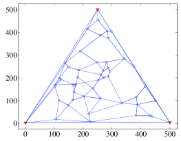
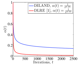
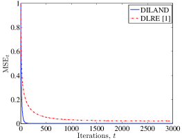
Figure 1: Distance noise only: Left: $N=50$ node network, $m=2$-D space, $m+1=3$, anchors and $M=47$ sensors. Center: Decreasing weight sequences, $\alpha(t)$, for DLRE and DILAND. Right: Normalized mean squared error for DLRE and DILAND.

In our second simulation, we keep the experimental setup, but include a zero-mean Gaussian random variable with unit variance as communication noise. We further assume that the communication links are active $90\%$ of the time. With this additional randomness in the localization algorithm, we cannot use the relaxed DILAND weights, but use the same weights given in Theorem 2 for both DLRE and DILAND, see Section III-C on a discussion on this choice. The network (along with appropriate triangulations) is shown in Fig. 2 (left.) Fig. 2 (center) shows the weights sequences chosen for DLRE and DILAND, whereas Fig. 2 (right) shows the normalized mean squared error.

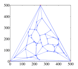
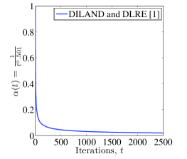
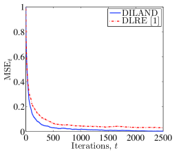
Figure 2: Distance noise, communication noise, and link failure: Left: $N=50$ node network, $m=2$-D space, $m+1=3$ anchors, and $M=47$ sensors. Center: Same weight sequence, $\alpha(t)$, for DLRE and DILAND. Right: Normalized mean squared error for DLRE and DILAND.

In both studies, we note that DLRE converges with a steady state error as is emphasized earlier, whereas, DILAND converges almost surely to the exact sensor locations. Furthermore, the simulations confirm that DILAND converges faster (faster convergence in the presence of all random phenomena is a consequence of refined distance measurements) because the square summability condition on $\alpha_{\mbox{\tiny DLRE}}(t)$ as required by DLRE is not required by $\alpha_{\mbox{\tiny DILAND}}(t)$.

V Conclusions

In this correspondence, we present a distributed localization algorithm, DILAND, that converges a.s. to the exact sensor locations when we have (i) communication noise, (ii) random link failures, and (iii) noisy distance measurements. We build on our earlier work, DLRE [1], that assumes that the noise on distance measurements results into a small signal perturbation of the system matrices; this perturbation is biased, in general. Due to this bias, there is a non-zero steady error in the location estimates of DLRE. With the additional assumption that the distance estimates at each iteration of DILAND converge a.s. to the exact distances, we show that the steady state error in the location estimates of DILAND is zero. We further show that if there is no communication noise and link failures, possible in some communication environments, the convergence rate of DILAND is faster than the convergence rate of DLRE. We provide simulations to assert the analytical results.

Appendix A Convergence of DILAND

We first summarize a relevant result that is needed for proving Theorem 3. The proof of this Lemma is in [9].

Lemma 1 (Lemma 18, [9])

Let the sequences $\{r_{1}(t)\}_{t\geq 0}$ and $\{r_{2}(t)\}_{t\geq 0}$ be given by

$$r_{1}(t)=\frac{a_{1}}{(t+1)^{\delta_{1}}},~{}~{}~{}~{}~{}r_{2}(t)=\frac{a_{2}}{(t+1)^{\delta_{2}}}$$ (24)

where $a_{1},a_{2},\delta_{2}\geq 0$ and $0\leq\delta_{1}\leq 1$. Then, if $\delta_{1}=\delta_{2}$, there exists $K>0$, such that, for non-negative integers, $s<t$,

$$0\leq\sum_{k=s}^{t-1}\left[\prod_{l=k+1}^{t-1}(1-r_{1}(l))\right]r_{2}(k)\leq K$$ (25)

Moreover, the constant $K$ can be chosen independently of $s,t$. Also, if $\delta_{1}<\delta_{2}$, then, for arbitrary fixed $s$,

$$\lim_{t\rightarrow\infty}\sum_{k=s}^{t-1}\left[\prod_{l=k+1}^{t-1}(1-r_{1}(l))\right]r_{2}(k)=0$$ (26)

We now prove the convergence of DILAND given by (16). Unless otherwise noted, the norm $\left\|\cdot\right\|$ refers to the standard Euclidean 2-norm. The following lemma shows that the DILAND iterations are bounded for all $t$.

Lemma 2

Consider the sequence of iterations in (16). We have

$$\mathbb{P}\left[\sup_{t\geq 0}\left\|\mathbf{x}^{j}(t)\right\|<\infty,~{}~{}1\leq j\leq m\right]=1.$$ (27)

In other words, the sequence $\{\mathbf{x}^{j}(t)\}_{t\geq 0}$ remains bounded a.s. for all $j$.

Proof.

We rewrite (16) as

$$\mathbf{x}^{j}(t+1) = (1-\alpha(t))\mathbf{x}^{j}(t)+\alpha(t)\left[\left(\mathbf{P}\left(\overline{\mathbf{d}}_{t}\right)+\mathbf{P}\left(\mathbf{d}^{\ast}\right)-\mathbf{P}\left(\mathbf{d}^{\ast}\right)\right)\mathbf{x}^{j}(t)+\mathbf{B}\left(\overline{\mathbf{d}}_{t}\right)\mathbf{u}^{j}\right],$$ (28)

$$= \left[(1-\alpha(t)I)+\alpha(t)\mathbf{P}(\mathbf{d}^{\ast})\right]\mathbf{x}^{j}(t)+\alpha(t)\left[\mathbf{P}(\overline{\mathbf{d}}_{t})-\mathbf{P}(\mathbf{d}^{\ast})\right]\mathbf{x}^{j}(t)+\alpha(t)\mathbf{B}(\overline{\mathbf{d}}_{t})\mathbf{u}$$ (29)

Since $\rho\left(\mathbf{P}(\mathbf{d}^{\ast})\right)<1$ (recall Theorem 1), it follows from the properties of linear operators on Banach spaces that there exists a norm $\left\|\cdot\right\|_{P}$ such that the corresponding induced norm of the linear operator $\mathbf{P}(\mathbf{d}^{\ast})$, satisfies

$$\left\|\mathbf{P}(\mathbf{d}^{\ast})\right\|_{P}=\max_{\mathbf{y}\neq\mathbf{0}}\frac{\left\|\mathbf{P}(\mathbf{d}^{\ast})\mathbf{y}\right\|_{P}}{\left\|\mathbf{y}\right\|_{P}}<1$$ (30)

Moreover, such a norm can be chosen to be equivalent to the Euclidean norm $\left\|\cdot\right\|$ (see, for example, [11]), i.e., there exist constants $c_{1},c_{2}>0$, such that, $c_{1}\left\|\cdot\right\|\leq\left\|\cdot\right\|_{P}\leq c_{2}\left\|\cdot\right\|$. In other words, $\left\|\cdot\right\|$ and $\left\|\cdot\right\|_{P}$ generate the same topology on the Euclidean space. Since $\alpha(t)\rightarrow 0$, we can choose $t_{0}$ sufficiently large, such that, $\alpha(t)<1,~{}~{}\forall t\geq t_{0}$. From the above construction, we have for, $t\geq t_{0}$,

$$\left\|(1-\alpha(t)\mathbf{I})+\alpha(t)\mathbf{P}(\mathbf{d}^{\ast})\right\|_{P}\leq 1-\alpha(t)+\alpha(t)\left\|\mathbf{P}(\mathbf{d}^{\ast})\right\|_{P}=1-\lambda^{\ast}\alpha(t)$$ (31)

where $0<\lambda^{\ast}\leq 1$. From $\overline{\mathbf{(B.3)}}$, we recall $\overline{\mathbf{d}}_{t}\rightarrow\mathbf{d}^{\ast}$ a.s. and from $\mathbf{P}(\cdot),\mathbf{B}(\cdot)$ being continuous functions of $\mathbf{d}_{t}$, we have

$$\mathbf{P}(\overline{\mathbf{d}}_{t})\rightarrow\mathbf{P}(\mathbf{d}^{\ast}),~{}~{}~{}\mbox{a.s.}~{}~{}~{}~{}~{}~{}~{}~{}~{}~{}\mathbf{B}(\overline{\mathbf{d}}_{t})\rightarrow\mathbf{B}(\mathbf{d}^{\ast}),~{}~{}~{}\mbox{a.s.}$$ (32)

Now fix a sample path $\omega$. There exists $t_{1}(\omega)$ sufficiently large, such that, for $0<\varepsilon<\lambda^{\ast}$, we have, if $t\geq t_{1}(\omega)$

$$\left\|\mathbf{P}(\overline{\mathbf{d}}_{t})-\mathbf{P}(\mathbf{d}^{\ast})\right\|_{P}\leq\varepsilon$$ (33)

Also, the a.s. convergence of $\mathbf{B}(\overline{\mathbf{d}}_{t})$, implies there exists $\lambda_{1}(\omega)$ such that $\left\|B(\overline{\mathbf{d}}_{t})\right\|_{P}\leq\lambda_{1}(\omega)$. Then, for $t\geq\max(t_{0},t_{1}(\omega))$

$$\left\|\mathbf{x}^{j}(t+1)\right\|_{P} \leq \left(1-\lambda^{\ast}\right)\left\|\mathbf{x}^{j}(t)\right\|_{P}+\varepsilon\alpha(t)\left\|\mathbf{x}^{j}(t)\right\|_{P}+\alpha(t)\lambda_{1}(\omega)\left\|\mathbf{u}^{j}\right\|_{P}$$ (34)

$$= \left(1-(\lambda^{\ast}-\varepsilon)\alpha(t)\right)\left\|\mathbf{x}^{j}(t)\right\|_{P}+\alpha(t)\lambda_{1}(\omega)\left\|\mathbf{u}^{j}\right\|_{P}$$

Let $t_{2}(\omega)=\max(t_{0},t_{1}(\omega))$, $a_{1}=\lambda^{\ast}-\varepsilon$, and $a_{2}(\omega)=\lambda_{1}(\omega)\left\|\mathbf{u}^{j}\right\|_{P}$. Continuing the above recursion, we have for $t\geq t_{2}(\omega)$

$$\left\|\mathbf{x}^{j}(t)\right\|_{P} \leq \left(\prod_{k=t_{2}(\omega)}^{t-1}(1-a_{1}\alpha(t))\right)\left\|\mathbf{x}(t_{2}(\omega))\right\|_{P}+\sum_{k=t_{2}(\omega)}^{t-1}\left[\left(\prod_{l=k+1}^{t-1}(1-a_{1}\alpha(l))\right)a_{2}\alpha(k)\right]$$ (35)

$$\leq \left\|\mathbf{x}(t_{2}(\omega))\right\|_{P}+\sum_{k=t_{2}(\omega}^{t-1}\left[\left(\prod_{l=k+1}^{t-1}(1-a_{1}\alpha(l))\right)a_{2}(\omega)\alpha(k)\right]$$

The second term falls under the purview of Lemma 1 in Appendix A with $\delta_{1}=\delta_{2}=\delta$, and we have

$$\sup_{t\geq 0}\left\|\mathbf{x}^{j}(t)\right\|_{P}\leq K(\omega)$$ (36)

for some $K(\omega)>0$. Since the above analysis holds a.s., we have $\mathbb{P}\left[\sup_{t\geq 0}\left\|\mathbf{x}^{j}(t)\right\|_{P}<\infty\right]=1$. The lemma then follows from the fact that the norms $\left\|\cdot\right\|$ and $\left\|\cdot\right\|_{P}$ are equivalent. In particular, boundedness in $\left\|\cdot\right\|$ is equivalent to boundedness in $\left\|\cdot\right\|_{P}$. ∎

We now present the proof of Theorem 3.

Proof of Theorem 3.

We use a comparison argument. To this end, consider the idealized update

$$\widetilde{\mathbf{x}}^{j}(t+1)=\left(1-\alpha(t)\right)\widetilde{\mathbf{x}}^{j}(t)+\alpha(t)\left[\mathbf{P}(\mathbf{d}^{\ast})\widetilde{\mathbf{x}}(t)+\mathbf{B}(\mathbf{d}^{\ast})\mathbf{u}^{j}\right]$$ (37)

It follows from Theorem 1 that, for $j=1,\ldots,m$,

$$\lim_{t\rightarrow\infty}\widetilde{\mathbf{x}}^{j}(t)=\left(\mathbf{I-P}(\mathbf{d}^{\ast})\right)^{-1}\mathbf{B}(\mathbf{d}^{\ast})\mathbf{u}^{j}.$$ (38)

Define the sequence $\{\mathbf{e}^{j}(t)=\mathbf{x}^{j}(t)-\widetilde{\mathbf{x}}^{j}(t)\}_{t\geq 0}$. We then have

$$\mathbf{e}^{j}(t+1)=\left(1-\alpha(t)\right)\mathbf{e}^{j}(t)+\alpha(t)\mathbf{P}(\mathbf{d}^{\ast})\mathbf{e}^{j}(t)+\alpha(t)\left(\mathbf{P}(\overline{\mathbf{d}}_{t})-\mathbf{P}(\mathbf{d}^{\ast})\right)\mathbf{x}^{j}(t)+\alpha(t)\left(\mathbf{B}(\overline{\mathbf{d}}_{t})-\mathbf{P}(\mathbf{d}^{\ast})\right)\mathbf{u}^{j}.$$ (39)

Recall the norm $\left\|\cdot\right\|_{P}$ introduced in the proof of Lemma 2. From (31), we have for $t\geq t_{0}$,

$$\left\|(1-\alpha(t)\mathbf{I})+\alpha(t)\mathbf{P}(\mathbf{d}^{\ast})\right\|_{P}\leq 1-\lambda^{\ast}\alpha(t)$$ (40)

where $0<\lambda^{\ast}\leq 1$. Now, fix a sample path ($\omega$). Consider $\tau>0$. By (32), there exists sufficiently large $t_{3}(\omega,\tau)$ such that

$$\forall t\geq t_{3}(\omega,\tau):\>\>\left\|\mathbf{B}(\overline{\mathbf{d}}_{t})-\mathbf{B}(\mathbf{d}^{\ast})\right\|_{P}\leq\tau,~{}~{}~{}~{}~{}~{}~{}\left\|\mathbf{P}(\overline{\mathbf{d}}_{t})-\mathbf{P}(\mathbf{d}^{\ast})\right\|_{P}\leq\tau$$ (41)

Define $t_{4}(\omega,\tau)=\max_{t_{0},t_{3}(\omega,\tau)}$. We then have for $t\geq t_{4}(\omega,\tau)$

$$\left\|\mathbf{e}^{j}(t+1)\right\|_{P} \leq \left\|(1-\alpha(t)I)+\alpha(t)\mathbf{P}(\mathbf{d}^{\ast})\right\|_{P}\left\|\mathbf{e}^{j}(t)\right\|_{P}$$

$$+ \alpha(t)\left\|\mathbf{P}(\overline{\mathbf{d}}_{t})-\mathbf{P}(\mathbf{d}^{\ast})\right\|_{P}\left\|\mathbf{x}^{j}(t)\right\|_{P}+\alpha(t)\left\|\mathbf{B}(\overline{\mathbf{d}}_{t})-\mathbf{B}(\mathbf{d}^{\ast})\right\|_{P}\left\|\mathbf{u}^{j}\right\|_{P}$$

$$\leq \left(1-\lambda^{\ast}\alpha(t)\right)\left\|\mathbf{e}^{j}(t)\right\|_{P}+\tau\alpha(t)K(\omega)+\tau\left\|\mathbf{u}^{j}\right\|_{P}$$

$$\leq \left(1-\lambda^{\ast}\alpha(t)\right)\left\|\mathbf{e}^{j}(t)\right\|_{P}+\tau\alpha(t)\left(K(\omega)+\left\|\mathbf{u}^{j}\right\|_{P}\right)$$ (43)

where $K(\omega)$ is defined in (36). Continuing the above recursion, we have for $t>t_{4}(\omega,\tau)$

$$\left\|\mathbf{e}^{j}(t)\right\|_{P}\leq\left(\prod_{k=t_{4}(\omega,\tau)}^{t-1}(1-\lambda^{\ast}\alpha(t))\right)\left\|\mathbf{e}^{j}(t_{4}(\omega,\tau))\right\|_{P}+\tau\sum_{k=t_{4}(\omega,\tau)}^{t-1}\left[\left(\prod_{l=k+1}^{t-1}(1-\lambda^{\ast}\alpha(l))\right)\left(K(\omega)+\left\|\mathbf{u}^{j}\right\|_{P}\right)\alpha(k)\right]$$ (44)

Using the inequality $1-\lambda^{\ast}\alpha(t)\leq e^{-\lambda^{\ast}\alpha(t)}$ for sufficiently small $\lambda^{\ast}\alpha(t)$, we have

$$\lim_{t\rightarrow\infty}\left(\prod_{k=t_{4}(\omega,\tau)}^{t-1}(1-\lambda^{\ast}\alpha(t))\right)\left\|\mathbf{e}^{j}(t_{4}(\omega,\tau))\right\|_{P}\leq\lim_{t\rightarrow\infty}e^{\left(-\lambda^{\ast}\sum_{k=t_{4}(\omega,\tau)}^{t-1}\alpha(t)\right)}\left\|\mathbf{e}^{j}(t_{4}(\omega,\tau))\right\|_{P}=0$$ (45)

The last step follows from the fact that $\sum_{k=t_{4}(\omega,\tau)}^{\infty}\alpha(t)=\infty$. From Lemma 1, we have

$$\sum_{k=t_{4}(\omega,\tau)}^{t-1}\left[\left(\prod_{l=k+1}^{t-1}(1-\lambda^{\ast}\alpha(l))\right)\left(K(\omega)+\left\|\mathbf{u}^{j}\right\|_{P}\right)\alpha(k)\right]\leq c_{4}(\omega)$$ (46)

Note, in particular, $c_{4}(\omega)$ is independent of $\tau$. We then have from (44)

$$\limsup_{t\rightarrow\infty}\left\|\mathbf{e}^{j}(t)\right\|_{P} \leq \limsup_{t\rightarrow\infty}\left(\prod_{k=t_{4}(\omega,\tau)}^{t-1}(1-\lambda^{\ast}\alpha(t))\right)\left\|\mathbf{e}^{j}(t_{4}(\omega,\tau))\right\|_{P}$$

$$+ \tau\limsup_{t\rightarrow\infty}\sum_{k=t_{4}(\omega,\tau)}^{t-1}\left[\left(\prod_{l=k+1}^{t-1}(1-\lambda^{\ast}\alpha(l))\right)\left(K(\omega)+\left\|\mathbf{u}^{j}\right\|_{P}\right)\alpha(k)\right]\leq\tau c_{4}(\omega).$$

Since (A) holds for arbitrary $\tau>0$, we have $\lim_{t\rightarrow\infty}\left\|\mathbf{e}^{j}(t)\right\|_{P}=0.$ The theorem then follows from the fact that this convergence to zero holds for $\omega$ a.s and from the equivalence of the norms $\left\|\cdot\right\|$ and $\left\|\cdot\right\|_{P}$. ∎

References

- [1] Usman A. Khan, Soummya Kar, and José M. F. Moura, “Distributed sensor localization in random environments using minimal number of anchor nodes,” IEEE Transactions on Signal Processing, vol. 57, no. 5, pp. 2000–2016, May 2009.
- [2] Usman A. Khan, Soummya Kar, Bruno Sinopoli, and José M. F. Moura, “Distributed sensor localization in Euclidean spaces: Dynamic environments,” in 46th Allerton Conference On Communication, Control, and Computing, Monticello, IL, Sep. 2008, pp. 361–366.
- [3] N. Patwari, Location estimation in sensor networks, Ph.D., University of Michigan–Ann arbor, 2005.
- [4] G. Springer, Introduction to Riemann Surfaces, Addison-Wesley, Reading, MA, 1957.
- [5] M. J. Sippl and H. A. Scheraga, “Cayley–Menger coordinates,” Proceedings of the National Academy of Sciences of U.S.A., vol. 83, no. 8, pp. 2283–2287, Apr. 1986.
- [6] T. S. Rappaport, Wireless communications: Principles and practice, Prentice Hall Inc., New Jersey, 1996.
- [7] N. Patwari, A. O. Hero III, M. Perkins, N. Correal, and R. J. O Dea, “Relative location estimation in wireless sensor networks,” IEEE Trans. on Signal Processing, vol. 51, no. 8, pp. 2137–2148, Aug. 2003.
- [8] M.B. Nevel’son and R.Z. Has’minskii, Stochastic Approximation and Recursive Estimation, American Mathematical Society, Providence, Rhode Island, 1973.
- [9] S. Kar, J. M. F. Moura, and K. Ramanan, “Distributed parameter estimation in sensor networks: Nonlinear observation models and imperfect communication,” Submitted for publication, see also http://arxiv.org/abs/0809.0009, Aug. 2008.
- [10] Soummya Kar and José M. F. Moura, “Distributed consensus algorithms in sensor networks with imperfect communication: Link failures and channel noise,” IEEE Transactions on Signal Processing, vol. 57, no. 1, pp. 355–369, January 2009.
- [11] H. M. Rodrigues and J. Sola-Morales, “A note on the relationship between spectral radius and norms of bounded linear operators,” Cadernos de matematica, vol. 9, pp. 61–65, May. 2008.