Integrated K-band spectra of old and intermediate-age globular clusters in the Large Magellanic Cloud ††thanks: Based on observation collected at the ESO Paranal La Silla Observatory, Chile, Prog. ID 078.B-0205
Current stellar population models have arguably the largest uncertainties in the near-IR wavelength range, partly due to a lack of large and well calibrated empirical spectral libraries. In this paper we present a project, which aim it is to provide the first library of luminosity weighted integrated near-IR spectra of globular clusters to be used to test the current stellar population models and serve as calibrators for the future ones. Our pilot study presents spatially integrated -band spectra of three old (10 Gyr) and metal poor ([Fe/H] –1.4), and three intermediate age (1 – 2 Gyr) and more metal rich ([Fe/H] –0.4) globular clusters in the LMC. We measured the line strengths of the Na I, Ca I and 12CO (2–0) absorption features. The Na I index decreases with the increasing age and decreasing metallicity of the clusters. The index, used to measure the 12CO (2–0) line strength, is significantly reduced by the presence of carbon-rich TP-AGB stars in the globular clusters with age 1 Gyr. This is in contradiction with the predictions of the stellar population models of Maraston (2005). We find that this disagreement is due to the different CO absorption strength of carbon-rich Milky Way TP-AGB stars used in the models and the LMC carbon stars in our sample. For globular clusters with age 2 Gyr we find index measurements consistent with the model predictions.
Key Words.:
Galaxies: Magellanic Clouds – Galaxies: star clusters – Galaxies: clusters: individual: NGC 1754, NGC 1806, NGC 2005, NGC 2019, NGC 2162, NGC 2173 – Stars: carbon1 Introduction
Since the 90’s, the interpretation of the integrated light of galaxies (in the nearby universe or at high redshift) heavily relies on evolutionary population synthesis (EPS) models. Such models were pioneered by Tinsley (1980) and the method has been seriously extended since then (e.g. Bruzual & Charlot 1993; Worthey 1994; Vazdekis et al. 1996; Fioc & Rocca-Volmerange 1997; Leitherer et al. 1999; Maraston 2005; Schiavon 2007). They are used to determine ages, element abundances, stellar masses, stellar mass functions, etc., of those stellar populations that are not resolvable into single stars with today’s instrumentation, i.e. most of the universe outside the Local Group. To build such EPS models we use simple stellar populations (SSP). There are two essential advantages of focusing on SSPs. First, SSPs can be reliably calibrated. They can be compared directly with nearby globular cluster (GC) data for which accurate ages and element abundances are independently known from studies of the resolved stars. This step is crucial to fix the stellar population model parameters that are used to describe model input physics and which cannot be derived from first principles (e.g., convection, mass loss and mixing). Second, SSPs can be used to build more complex stellar systems. Systems made up by various stellar generations can be modelled by convolving SSPs with the adopted star formation history (e.g. Kodama & Arimoto 1997; Bruzual & Charlot 2003). Models describing accurately the integrated light properties, including medium to high resolution spectra and/or line-strength indices, are and will be our main tool to investigate and analyse the star-formation history over cosmological time-scales.
This approach has worked well in the optical spectroscopic regime and has led to well calibrated models (e.g. Thomas et al. 2003; Bruzual & Charlot 2003; Maraston 2005). With the application of such models to observed spectra we derive reasonable estimates of the main stellar population parameters (age, chemical composition and M/L ratio) in the nearby universe (e.g., Kuntschner 2000; Trager et al. 2000; Thomas et al. 2005; Cappellari et al. 2006; Sánchez-Blázquez et al. 2007) as well as at higher redshifts (e.g., Bernardi et al. 2005; Maraston 2005; Sánchez-Blázquez et al. 2009). Of course, uncertainties remain due to the degeneracy of age and metallicity effects in the optical wavelength range (e.g., Worthey 1994). The integrated near-IR light in stellar populations with ages 1 Gyr is dominated by one stellar component, cool giant stars, whose colour and line indices are mainly driven by one parameter: metallicity (Frogel et al. 1978). Near-IR colours and indices also have the advantage of being more nearly mass-weighted, i.e. the near-IR mass-to-light ratio is closer to one (see e.g., Worthey 1994). So, by combining the optical as well as near-IR information one can resolve the currently remaining degeneracies between age and chemical composition, present in the models, and hope to gain a better understanding of star-formation histories. However, currently available stellar population models have arguably the largest uncertainties in the near-IR and thus it is of paramount importance to provide high-quality observational data to validate and improve the state-of-the-art models.
Globular clusters in the Local Group are an ideal laboratory for this project since ample information from studies of the resolved stars is available. Yet, integrated spectroscopic observations of the Galactic GCs in the near-IR are very challenging due to their large apparent sizes on the sky. The Large Magellanic Cloud (LMC) and its globular cluster system, located about 50 kpc away, is a much better observational choice. It shows evidence for a very complex and still ongoing star formation activity. The LMC GCs have an advantage (for the scope of this project) with respect to Galactic GCs - they span a larger range in ages. Studies of the LMC globular cluster system show one old component with age 10 Gyr. After this time there was a ”dark age” with just one cluster formed before a new burst of cluster formation that has started around Gyr ago (Da Costa 1991). A disadvantage is their lower metallicity.
| Name | UT date | SWB | Age | [Fe/H] | ||
|---|---|---|---|---|---|---|
| (1) | (2) | (3) | (4) | (5) | (6) | (7) |
| NGC 1754 | 2006 Nov 18 | 11.57 | 0.75 | VII | 10 | -1.42a, -1.54b |
| NGC 2005 | 2006 Nov 29 | 11.57 | 0.73 | VII | 10 | -1.35a, -1.92b, -1.80c, -1.33d |
| NGC 2019 | 2006 Dec 10 | 10.86 | 0.76 | VII | 10 | -1.23a, -1.18b, -1.37c, -1.10d |
| NGC 1806 | 2006 Dec 06 | 11.10 | 0.73 | V | 1.1 | -0.23b, -0.71e |
| NGC 2162 | 2006 Dec 05 | 12.70 | 0.68 | V | 1.1 | -0.23b, -0.46f |
| NGC 2173 | 2006 Dec 06 | 11.88 | 0.82 | V-VI | 2 | -0.24b, -0.42f, -0.51g |
The goal of this project is to provide an empirical near-IR library of spectra for integrated stellar populations with ages 1 Gyr, which will be used to verify the predictions of current SSP models in the near-IR wavelength range. Here we present the results from a pilot study of -band spectra of 6 globular clusters in the LMC. The analysis of their and -band spectra will be discussed in a separate paper. This paper is organised as follows: in Sect. 2 we give details about the sample selection and the observing strategy. Sect. 3 is devoted to the observations and data reduction. In Sect. 4 we discuss the cluster membership of the stars in our sample, in Sect. 5 we describe the near-IR index measurement procedures. In Sect. 6 we make a comparison between the currently available stellar population models in the near-IR with our data, discuss the observed disagreements, and give potential explanations. Finally, in Sect. 7 we give our concluding remarks.
2 Sample selection and observational strategy
Due to our interests in the application of SSP models to the integrated light of early-type galaxies, we restricted our sample in this pilot study to intermediate age (1–2 Gyr) and old ( 10 Gyr) clusters. The sample was selected from the Bica et al. (1996, 1999) catalogues by choosing the SWB class (Searle et al. 1980) to be V, VI or VII. In this way we ensured that the target systems will have ages Gyr. We further required the clusters to be bright () and reasonably concentrated (effective radius ). Where no literature data were available, the concentration was checked by eye on DSS images. Another selection criterion was the availability of auxiliary data, because we needed detailed information on age and chemical composition. All of the selected clusters have HST/WFPC2 and/or ACS imaging (e.g. Olsen et al. 1998; Mackey & Gilmore 2003), integrated optical spectroscopy, and spectra of individual giant stars (e.g. Olszewski et al. 1991; Beasley et al. 2002; Johnson et al. 2006; Mucciarelli et al. 2008). We can also benefit from near-IR studies, both imaging and spectroscopy, of the giant stars in these clusters (e.g. Frogel et al. 1990; Mucciarelli et al. 2006), as well as of photometry (Persson et al. 1983; Mucciarelli et al. 2006; Pessev et al. 2006). Taking into account the above criteria we selected six clusters as targets for this pilot project, aiming at validating the strategy for observations and analysis (see Table 1). Three of the clusters are metal poor (mean [Fe/H] ) and have ages of more than 10 Gyr. The other three are more metal rich (mean [Fe/H] ) and younger, with ages between 1 and 2 Gyr. In the literature there are different age and metallicity estimates for the clusters in our sample, depending on the methods used. Here we listed the ages based on SWB types, given in Frogel et al. (1990) and a compilation of metallicities, obtained from the literature. A summary of the clusters’ properties is given in Table 1.
Integrated spectra of clusters with less than are likely to be dominated by statistical fluctuations in the number of bright AGB and RGB stars (e.g. Renzini 1998, for more details see Sect. 4). These particular phases of the stellar evolution are one of the main contributors to the integrated light of an intermediate age stellar population in the near-IR (e.g. Maraston 2005). To sample as much of the cluster light in a reasonable observing time, we made a mosaic of 3 3 VLT/SINFONI pointings ( per pointing with a 025 spatial sampling) centred on each cluster. We estimated the total light sampled by the central mosaic for all clusters using the following equation and the 20 radius aperture -band photometry:
| (1) |
where is the observed -band integrated magnitude of the cluster, is the adopted distance modulus to the LMC (van den Bergh 1998; Alves et al. 2002; Alves 2004; Borissova et al. 2004), is the extinction towards each cluster (Zaritsky et al. 1997), is the -band absolute magnitude of the Sun (Cox 2000). The bolometric correction is applied in order to obtain the total bolometric luminosity of the cluster. It depends on the adopted age and metallicity of the stellar populations. In our case it is 0.6 for the group of the old and metal poor clusters (NGC 1754, NGC 2005 and NGC 2019) and 0.3 for the more metal rich and intermediate age clusters NGC 1806, NGC 2162 and NGC 2173 (Maraston 1998, 2005). For all but two clusters we found that the sampled luminosity is (see Table 2). Only the young clusters NGC 2162 and NGC 2173 are at the limit or bellow this value.
In order to maximise the statistical probability of getting the majority of the RGB and AGB stars, we observed, in addition to the central mosaics, up to 9 of the brightest stars surrounding each cluster and outside of the central mosaic. Their selection was based on colour-magnitude diagrams from the 2MASS Point Source Catalogue (Skrutskie et al. 2006) of all the stars with reliable photometry and located inside the tidal radius of each cluster ( taken from McLaughlin & van der Marel 2005, see Table 2). We selected the stars with and as an initial separation criterion from the LMC field population.
The inclusion of these additional bright stars in our sample has a twofold purpose. The original idea, as described above, was to provide a better sampling of the integrated cluster light by in- or excluding these bright stars (after a careful decision process, based on kinematical and chemical composition assumptions). Second, the stars, which turn out not to be members of any cluster, are representative for the LMC field star population in the vicinity of our GCs. Thus we obtained an independent field AGB stars sample for comparison with the globular clusters. The main properties of these additional stars are listed in Table 3.
| Name | Rint | ||||||||
|---|---|---|---|---|---|---|---|---|---|
| (1) | (2) | (3) | (4) | (5) | (6) | (7) | (8) | (9) | (10) |
| NGC 1754 | 112 | 1429 | 9.01 | 10.21 | 20 | – | – | – | |
| NGC 2005 | 865 | 988 | 8.92 | 9.80 | 20 | – | – | – | |
| NGC 2019 | 972 | 1216 | 8.31 | 9.21 | 20 | – | – | – | |
| NGC 1806 | – | – | 7.57 | 9.19 | 100 | 7.076 | 1.055 | 0.271 | |
| NGC 2162 | 2137 | 1972 | 9.65 | 11.18 | 120 | 9.071 | 1.253 | 0.372 | |
| NGC 2173 | 3435 | 3935 | 8.86 | 10.69 | 60 | 9.050 | 1.033 | 0.297 |
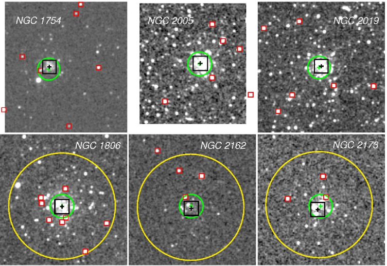
In Fig. 1 we show the 2MASS -band images, obtained from the 2MASS Extended Source Catalogue of our globular cluster sample. The black cross and box on each cluster image match the centre and the extent of the SINFONI mosaic coverage, respectively. The red squares mark the additional bright stars, observed around the clusters within the region of the 2MASS image. The green circle and cross show the centre and 20 radius aperture, which Pessev et al. (2006) used to obtain integrated magnitudes for each cluster. These authors have used near-IR images from the 2MASS Extended Source Catalogue and have performed photometry with different aperture sizes after correcting for the extinction and LMC field population. Mucciarelli et al. (2006) have used ESO 3.5 m NTT/SOFI images to provide integrated near-IR magnitudes for half of the globular clusters in our sample after decontaminating from the LMC field population and correcting for the extinction and completeness. The large yellow circles show their 90 fixed radius aperture. We used these photometric studies to compare our spectroscopy with integrated colours and magnitudes. There is a good agreement between the centres of our SINFONI observations and the photometry studies, however, in the case of the sparsely populated cluster NGC 2173 the offset is 17″ (in all other cases this offset is smaller than 5″).
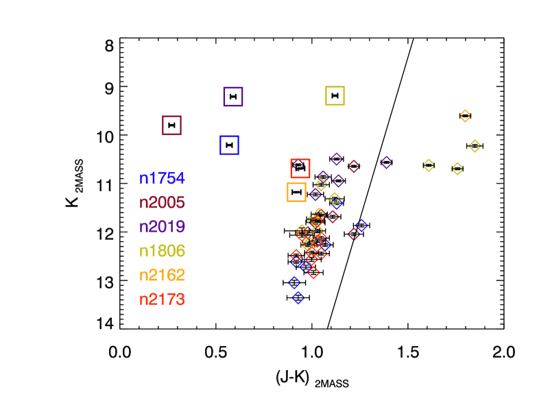
A summary colour-magnitude diagram for all observed objects in our sample, stars and central mosaics, is shown in Fig. 2. For the and -band magnitude of the central mosaics we adopted the 20 radius aperture photometry of Pessev et al. (2006), which, as shown on Fig. 1, matches reasonably well our central mosaics. The selected in addition bright stars outside the central mosaics are denoted with diamond symbols. Their photometry comes from the 2MASS Point Source Catalogue and magnitudes were dereddened following the same method as Pessev et al. (2006) – extinction values were obtained from the Magellanic Clouds Photometric Survey (Zaritsky et al. 1997) and adopting the extinction law of Bessell & Brett (1988). The slanted line in this figure represents the separation between oxygen- and carbon-rich giant stars of Cioni et al. (2006). According to this criterion we have five carbon rich stars in our sample.
3 Observations and data reduction
3.1 Observations
The observations of the selected globular clusters and stars were obtained in service mode in the period October – December 2006 (Prog. ID 078.B-0205, PI: Kuntschner). We used the integral field unit spectrograph SINFONI (Eisenhauer et al. 2003; Bonnet et al. 2004), which is mounted in the Cassegrain focus of Unit Telescope 4 (Yepun) on VLT at Paranal La Silla Observatory. Its gratings are in the near-IR spectral domain (1 – 2.5 m). We used the -band grating, which covers the wavelength range from 1.95 to 2.45 m at a dispersion of /pix. The spectral resolution around the centre of the wavelength range is R (6.2 Å FWHM), as measured from arc lamp frames. The largest single pointing with SINFONI covers , which is too small even for the most compact LMC clusters due to their relatively large apparent sizes on the sky. To sample at least one effective radius of our targets we decided to use a mosaic of the largest FoV of SINFONI, thus covering the central for each cluster. Given the goal to sample the total light, and not to get the best possible spatial resolution, all the observations were performed in natural seeing mode, i.e. with no adaptive optics correction. The integration time was chosen based on the requirement to achieve a signal-to-noise ratio of at least 50 in the final integrated spectra. The exposure time for one pointing of the mosaic was 150 s, divided into three integrations of 50 s, dithered by to reject bad pixels. With the short integration time we could reliably measure and subtract the very bright and variable near-IR night sky using the data reduction procedure as described in the next section.
In order to correct for the effects of the night sky, we observed empty sky regions very close in time and space to our scientific observations, in a SOOOS sequence for each mosaic pointing (S - sky integration, O - object). For the additional bright stars outside the central mosaic we used the same sequence, but with shorter integration times of 10 s per individual integration, leading to a total on source time of 30 s. The sky fields for each cluster were located outside its tidal radius (see Table 2) and were checked by eye on 2MASS images to be devoid of bright stars. The total execution time for the longest observing sequence did not exceed 1.5 hours. This ensured that the telluric correction, derived from the telluric stars, observed after each cluster and additional bright stars sequence (see Table 4) would be sufficiently accurate. The telluric stars were observed at similar airmass as the clusters.
| Name | R. A. | Dec. | Notes | Cluster | |||
|---|---|---|---|---|---|---|---|
| (1) | (2) | (3) | (4) | (5) | (6) | (7) | (8) |
| 2MASS J04540127-7026341 | 04 54 01.27 | -70 26 34.17 | 11.40 | 1.13 | 1.2080.013 | NGC 1754 | |
| 2MASS J04540771-7024398 | 04 54 07.72 | -70 24 39.88 | 11.86 | 1.26 | 1.2230.021 | ” | |
| 2MASS J04543522-7027503 | 04 54 35.22 | -70 27 50.36 | 12.26 | 1.07 | 1.1430.015 | ” | |
| 2MASS J04542864-7026142 | 04 54 28.64 | -70 26 14.23 | 12.62 | 0.91 | 1.1120.018 | ” | |
| 2MASS J04540935-7024566 | 04 54 09.35 | -70 24 56.66 | 12.73 | 0.96 | 1.0880.021 | ” | |
| 2MASS J04541188-7028201 | 04 54 11.88 | -70 28 20.13 | 13.04 | 0.91 | 1.1770.030 | ” | |
| 2MASS J04540536-7025202 | 04 54 05.36 | -70 25 20.20 | 13.36 | 0.93 | 1.1220.029 | ” | |
| 2MASS J05302221-6946124 | 05 30 22.21 | -69 46 12.48 | 10.65 | 1.21 | 1.2580.008 | NGC 2005 | |
| 2MASS J05300708-6945327 | 05 30 07.08 | -69 45 32.73 | 11.66 | 1.04 | 1.2130.012 | ” | |
| 2MASS J05295466-6946014 | 05 29 54.66 | -69 46 01.44 | 11.68 | 1.12 | 1.2460.010 | ” | |
| 2MASS J05300704-6944031 | 05 30 07.04 | -69 44 03.11 | 11.80 | 1.03 | 1.2510.010 | ” | |
| 2MASS J05300360-6944311 | 05 30 03.60 | -69 44 31.18 | 12.02 | 0.97 | 1.2160.013 | ” | |
| 2MASS J05295822-6944445 | 05 29 58.22 | -69 44 44.59 | 12.05 | 1.22 | 1.2330.016 | ” | |
| 2MASS J05320670-7010248 | 05 32 06.70 | -70 10 24.84 | 10.49 | 1.13 | 1.1360.014 | NGC 2019 | |
| 2MASS J05313862-7010093 | 05 31 38.62 | -70 10 09.35 | 10.56 | 1.39 | 1.1960.017 | C | ” |
| 2MASS J05315232-7010083 | 05 31 52.32 | -70 10 08.39 | 10.61 | 0.94 | 1.2000.016 | ” | |
| 2MASS J05321152-7010535 | 05 32 11.52 | -70 10 53.52 | 10.87 | 1.06 | 1.1760.018 | ” | |
| 2MASS J05321647-7008272 | 05 32 16.47 | -70 08 27.26 | 10.95 | 1.13 | 1.1830.016 | ” | |
| 2MASS J05320418-7008151 | 05 32 04.18 | -70 08 15.15 | 11.22 | 1.02 | 1.2040.024 | ” | |
| 2MASS J05021232-6759369 | 05 02 12.32 | -67 59 36.92 | 10.23 | 1.84 | 1.0510.013 | +,C | NGC 1806 |
| 2MASS J05020536-6800266 | 05 02 05.36 | -68 00 26.69 | 10.63 | 1.61 | 1.1390.015 | +,C | ” |
| 2MASS J05015896-6759387 | 05 01 58.96 | -67 59 38.76 | 10.69 | 1.76 | 1.0650.013 | +,C | ” |
| 2MASS J05021623-6759332 | 05 02 16.23 | -67 59 33.22 | 11.02 | 1.06 | 1.2110.012 | + | ” |
| 2MASS J05021870-6758552 | 05 02 18.70 | -67 58 55.20 | 11.32 | 1.11 | 1.2670.015 | + | ” |
| 2MASS J05021846-6759048 | 05 02 18.46 | -67 59 04.82 | 11.74 | 1.00 | 1.2430.018 | ” | |
| 2MASS J05021121-6759295 | 05 02 11.21 | -67 59 29.54 | 11.97 | 0.96 | 1.1970.026 | ” | |
| 2MASS J05021137-6758401 | 05 02 11.37 | -67 58 40.15 | 11.98 | 1.02 | 1.1990.023 | ” | |
| 2MASS J06002748-6342222 | 06 00 27.48 | -63 42 22.29 | 9.60 | 1.80 | 1.0750.012 | +,C | NGC 2162 |
| 2MASS J06003156-6342581 | 06 00 31.56 | -63 42 58.14 | 11.64 | 1.03 | 1.2020.011 | + | ” |
| 2MASS J06003316-6342131 | 06 00 33.16 | -63 42 13.18 | 12.24 | 0.99 | 1.1970.016 | + | ” |
| 2MASS J06003869-6341393 | 06 00 38.69 | -63 41 39.37 | 12.26 | 0.99 | 1.1840.020 | ” | |
| 2MASS J05563892-7258155 | 05 56 38.92 | -72 58 15.52 | 11.77 | 1.03 | 1.2270.012 | NGC 2173 | |
| 2MASS J05575667-7258299 | 05 57 56.67 | -72 58 29.91 | 12.07 | 0.95 | 1.1660.014 | + | ” |
| 2MASS J05570233-7257449 | 05 57 02.33 | -72 57 44.95 | 12.13 | 1.04 | 1.1590.016 | ” | |
| 2MASS J05575784-7257548 | 05 57 57.84 | -72 57 54.89 | 12.18 | 1.03 | 1.2030.016 | + | ” |
| 2MASS J05563368-7257402 | 05 56 33.68 | -72 57 40.28 | 12.43 | 1.00 | 1.1460.016 | ” | |
| 2MASS J05581142-7258328 | 05 58 11.42 | -72 58 32.87 | 12.45 | 1.04 | 1.1540.019 | + | ” |
| 2MASS J05583257-7258499 | 05 58 32.57 | -72 58 49.90 | 12.48 | 0.92 | 1.1360.015 | ” | |
| 2MASS J05572334-7256006 | 05 57 23.34 | -72 56 00.66 | 12.56 | 1.01 | 1.2270.019 | ” | |
| 2MASS J05565761-7254403 | 05 56 57.61 | -72 54 40.38 | 12.84 | 1.01 | 1.1690.020 | ” |
3.2 Basic data reduction
An overview of the different data reduction steps and their results is shown in Fig. 3. There we show a sequence of a raw spectrum, then the sky subtracted spectrum, the telluric correction spectrum, and the final, fully reduced spectrum. More details about the data reduction can be found in Lyubenova (2009). Here we briefly discuss the most important steps.
The basic data reduction was performed with the ESO SINFONI Pipeline v. 1.9.2. Calibration products such as distortion maps, flat fields and bad pixel maps, were obtained with the relevant pipeline tasks (“recipes”). To reduce the clusters and additional star data, we divided each observing sequence into cluster frames (27 object plus 10 sky exposures) and star frames (3 star exposures plus one sky per star). This was needed due to the different integration times for these two sub-sets. We also preferred to reduce each mosaic pointing separately and combine the nine later. In this way we controlled the quality of each on-source frame sky correction and where needed we tuned some of the parameters in the pipeline. In summary, we have fed the sinfo_rec_jitter recipe with data sets, consisting of one mosaic pointing (3 on source integrations plus 2 bracketing “skies”) and the needed calibration files. Then the recipe extracts the raw data, applies distortion, bad pixels and flat-field corrections, wavelength calibration, and stores the combined sky-subtracted spectra in a 3-dimensional data cube. The same pipeline steps were also used to reduce the observations of the additional bright stars and telluric stars.
The main difficulty during the sky correction arises from the fact that our observations were sky dominated, combined together with the small amount of flux in some of the frames. For these cases we found that by appropriately setting the parameters that indicate the edges of the object spectrum location (--skycor-llx, --skycor-lly, --skycor-urx and --skycor-ury), we could achieve a good sky correction.

3.3 Telluric corrections
The next data reduction step was to remove the absorption features originating in the Earth’s atmosphere. These features are especially deep in the blue part of the -band (blue-wards of 2.1 m). For this purpose we observed after each science target a telluric star, which is of hotter spectral type (usually A – B dwarfs, see Table 4). Since these stars are hot stars, we know that their continuum in the -band is well approximated by the Rayleigh-Jeans part of the black body spectrum, associated with their effective temperature. They show only one prominent feature, the hydrogen Brackett absorption line at m. For each telluric star spectrum first we modelled this line with a Lorentzian profile, with the help of the IRAF task splot, and then subtracted the model from the star’s spectrum. Then we divided the cleaned star spectrum by a black body spectrum with the same temperature as the star to remove its continuum shape. Thus we obtained a normalised telluric spectrum. The last step before applying it to the science spectra was to scale and shift in the dispersion direction each telluric spectrum for each data cube by a small amount ( 0.5 pix, 1 pix = 2.45 ) to minimise the residuals of the telluric lines (for more details about this procedure see Silva et al. 2008). After that each individual cluster mosaic and star data cube was divided by the so optimised telluric spectrum. In this way we achieved also a relative flux calibration.
One telluric star, HD 44533, used for the telluric correction of NGC 2019 and its surrounding stars, has an unusual shape of the Brackett line. It seems to have also some emission together with the absorption. To remove it, we interpolated linearly the region between 2.1606 and 2.1706 m. In this region there are not many strong telluric lines, but this interpolation will reflect in an imperfect correction of the science spectra for this cluster at the above wavelengths. However, none of the spectral features of interests for this study reside in this wavelength range.
| Name | Cluster | R. A. | Dec. | SpT |
|---|---|---|---|---|
| (1) | (2) | (3) | (4) | (5) |
| HD 40624 | NGC 1754 | 05:54:56.97 | -65:53:00.65 | A0V |
| HD 43107 | NGC 2005 | 06:08:44.26 | -68:50:36.27 | B8V |
| HD 44533 | NGC 2019 | 06:14:41.94 | -73:37:35.44 | B8V |
| HD 42525 | NGC 1806 | 06:06:09.38 | -66:02:22.63 | A0V |
| HD 45796 | NGC 2162 | 06:24:55.79 | -63:49:41.32 | B6V |
| HD 46668 | NGC 2173 | 06:27:13.64 | -73:13:42.08 | B8V |
3.4 Cluster light integration
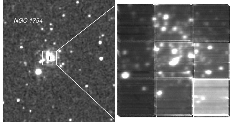
As a result from the previous data reduction steps we obtained fully calibrated data cubes for each SINFONI pointing, where the signatures of the instrument and the night sky are removed as well as possible. During the next step we reconstructed the full mosaic of each cluster. For example, Fig. 4 shows the reconstructed image of the cluster NGC 1754, together with a 2MASS -band image for comparison. In this image we still see the imprints of the edges of the individual mosaic tiles. On both images, the 2MASS and even better on the SINFONI image, we see individual stars, which can be extracted and studied separately.
However, here we are interested in luminosity weighted, integrated spectra for each cluster, to compare with stellar population models. To construct one integrated spectrum per cluster we first estimated the noise level in each reconstructed image from the mosaic data cube. We considered this noise is due to residuals after the sky background correction. Thus we computed the median residual sky noise level and its standard deviation, after clipping all data points with intensities more than 3 (assuming that these are the pixels, which contain the star light from the cluster). After that we selected all spaxels, which have intensity more than three times the standard deviation above the median residual sky noise level. We summed them up and normalised to 1 s exposure time. In some of the spectra (NGC 1754 and NGC 2019), we still suffered from sky line residuals, originating from the addition of imperfectly sky corrected spaxels (this may happen with intrinsically low intensity spaxels). In these cases we interpolated the contaminated regions.
Our observations were carried out in service mode with constraint sets allowing seeing up to 2. For the individual stars this led to a failure of the standard pipeline recipe while extracting 1D spectra. Moreover in some cases in the field-of-view there were also other stars. Thus we decided to manually control the selection of star light spaxels. We used the same method as for the central clusters mosaics to obtain the spectra of the additional stars.
3.5 Error handling
The SINFONI pipeline does not provide error estimates, which carry information about the error propagation during the different data reduction procedures. Thus we have to use empirical ways of computing the errors. For this purpose we derived a wavelength dependent signal-to-noise ratio (S/N) for each cluster integrated spectrum using the empirical method described by Stoehr et al. (2007). We computed the S/N in 200 pixels width bins from the science spectra (corresponding to 0.049 m wavelength intervals). Then we fitted a linear function to the S/N values in the range 2.1 – 2.4 m where all of the spectral features of interest reside. The error spectrum for each cluster and star was derived by dividing the science spectrum by the so prepared S/N function. The selection of the bin width was made after experimenting with a few smaller and larger values. In the case of bin widths of 50 or 100 pixels (0.01225 or 0.0245 m, respectively), the S/N function becomes very noisy. Choosing wider, 300 or 400 pixels bins flattens the features of the S/N function. In general the S/N decreases with increasing wavelength. This is due to the combination of the spectral energy distribution and the instrument + telescope sensitivity. The mean S/N around 2.3 m is larger than 50 for the integrated spectra over the central mosaics of the clusters and in the range 10 – 40 for the individual stars, depending on their magnitude. The S/N estimate for carbon star spectra is a lower limit due to the numerous absorption features due to carbon based molecules, which are interpreted by the routine as noise. The error spectra were used to estimate the errors of the index measurements, as shown in the plots in this paper.
4 Additional bright AGB stars – cluster members or not?
As discussed in Sect. 2 one of the main problems, when one tries to compile a representative integrated spectrum of a globular cluster, is the stochastic sampling of bright AGB stars for clusters with modest luminosities. As an example, Renzini (1998) shows that a stellar cluster with , solar metallicity and age of 15 Gyr will have about red giant branch stars (RGB), early asymptotic giant branch stars (E-AGB), and only 2 thermally pulsating asymptotic giant branch (TP-AGB) stars. The latter stellar evolutionary phase is particularly important for intermediate age stellar populations of 1 Gyr, since up to 80% of their total -band light originates there (e.g. Maraston 2005, and references therein). In general the old clusters (NGC 1754, NGC 2005 and NGC 2019) are massive and well concentrated, with half-light radii sampled with our SINFONI central mosaics. Therefore our observations sample 50% of the total bolometric light coming from these clusters, and in all cases we sample at least .
However, we were not performing that well with the intermediate age clusters, where for two of them, NGC 2162 and NGC 2173, we sample even less than (see Table 2). Our observations are intrinsically affected by statistical fluctuations in the number of bright stars, due to the modest luminosities of the young clusters. These clusters are less massive and less concentrated than other clusters in our sample. In the more massive clusters, mass segregation has likely caused a central concentration of the more massive main sequence progenitors of the observed AGB stars than the lower mass background stars that have not yet evolved off the main sequence. In the younger, less massive clusters, mass segregation has likely been less efficient. Hence, the AGB progenitors will be less centrally concentrated relative to other unevolved stars. In turn, this implies that AGB stars may be found at larger projected radii in lower mass clusters than in higher mass clusters.
In order to have integrated spectra as representative of our globular clusters, including the most important stellar evolutionary phases, we observed a number of additional bright stars with near-IR colours and magnitudes in the range expected for RGB and AGB stars, as explained in the previous sections. After probing their membership, we added some of them to the central mosaics cluster light to obtain the final integrated spectra, as explained bellow. We have to note that we have added only integer numbers of bright stars. This is useful when one aims to obtain a representative spectrum for a given globular cluster, what was our goal in this project. In order to achieve an integrated spectrum representative of a full stellar population with a given age and chemical composition, where stochastics does not play a role, one should also consider adding fractional number of bright AGB stars.
The first criterion for cluster membership of the stars is the proximity to the cluster centre, but a LMC field star might also have a relatively nearby position due to projection effects. The second possibility is to explore the radial velocities of the nearby stars and the cluster under study. For this purpose we also need to know the observed velocity dispersions of the stars in the clusters. Due to the low velocity resolution of our observations we used data from the literature. For the old clusters (NGC 1754, NGC 2005 and NGC 2019) we took these values from the study of Dubath et al. (1997). They have measured core velocity dispersions from integrated optical spectra, covering the central of each cluster. The values are 7. 8 3.0 for NGC 1754, 8.1 1.3 for NGC 2005 and 7.5 1.3 for NGC 2019. For the intermediate-age clusters we could not find similar observed velocity dispersions in the literature, thus we used the predicted line-of-sight velocity dispersion at the centre of the cluster by McLaughlin & van der Marel (2005). The numbers are 1.1 for NGC 2162 and 2.0 for NGC 2173. We did not find a similar estimate for NGC 1806, so we used a conservative upper limit of 8 .
4.1 Old clusters
In the case of the three old clusters, NGC 1754, NGC 2005 and NGC 2019 we cannot exclude any star around any cluster, because their velocities are consistent with cluster membership. This is due to the insufficient velocity resolution of our observations. However, some of the brightest stars that we have observed are located closer to the tidal radii of the clusters, than to their centres. This is not expected for old clusters, which have already undergone a core collapse and have their most massive stars concentrated towards the centre of the cluster. Indeed, Mackey & Gilmore (2003) classify the old clusters in our sample as potential post-core-collapse clusters, due to the very well expressed power-law cusps in their centres. Moreover, in Fig. 2 the colours of the central mosaics are much bluer than the colours of the additional bright stars around the old clusters. Santos & Frogel (1997) point out that very young and not massive clusters can be systematically bluer than average due to stochastic sampling of the IMF. However, the integrated spectra of the three old globular clusters discussed here are sampling several times and have ages of 10 Gyr. In this regime the simulations of Santos & Frogel (1997) predict much less fluctuations in the colour than the observed difference between the central mosaics and the additional stars. This additionally led us to the conclusion that these stars are not likely to be cluster members. In the following we considered them as members of the LMC field population. The bright star marked with a red square just outside the SINFONI field-of-view for NGC 1754 in Fig. 1 might be a cluster member, but the S/N of its spectrum is too low ( 10) and adding it to the final integrated cluster spectrum would not increase the total S/N.
4.2 Intermediate age clusters
This sub-sample includes the clusters NGC 1806, NGC 2162 and NGC 2173. The last two of them are poorly populated as seen in near-IR light, visible from Fig. 1, so in their cases the potential inclusion of additional bright stars to the central mosaic is very important for the total cluster light sampling. A detailed photometric study of the RGB and AGB stars in these clusters is available from Mucciarelli et al. (2006). Based on near-IR colour-magnitude diagrams and after decontamination from the field population, they report several stars in these evolutionary phases, as well as their luminosity contribution to the total light of the clusters. They consider all stars brighter than , which represents the level of the RGB tip (Ferraro et al. 2004), and between 0.85 and 2.1 to be AGB stars.
The AGB stars separate in oxygen rich (M-stars) and carbon rich (C-stars). An AGB star becomes C-rich, when the amount of dredged up carbon into the stellar envelope exceeds the amount of oxygen. Then all the oxygen is bound into CO molecules. The remaining carbon is used to form CH, CN and C2 molecules. This process is more effective in more metal poor stellar populations, thus they are expected to have more C-stars (Maraston 2005). C-stars can contribute up to 60% of the total luminosity of metal-poor clusters (Frogel et al. 1990). Another important statement that Frogel et al. (1990) make is that C and M type stars are found both in clusters and in the LMC field. Thus it is very difficult to separate intermediate age globular cluster stars from the field population.
However, the LMC field carbon stars contamination is not expected to be significant at the locations of the globular clusters in our sample. The upper limits, according to the carbon stars frequency maps of Blanco & McCarthy (1983) are of the order of 0.05 to 0.7 C-type stars for an area with a radius of 100.
NGC 1806: This cluster is relatively rich in stars, as seen on Fig. 1. However, there is a lack of information about its spectral properties. So far, studies of the stellar populations have been made mainly with photometric methods (e.g. Frogel et al. 1990; Dirsch et al. 2000; Mucciarelli et al. 2006; Mackey et al. 2008), and two bright cluster stars have been observed by Olszewski et al. (1991) to spectroscopically estimate the metallicity of the cluster (see Table 1). Moreover, there is neither information about its dynamical properties in the literature, nor information about its bounds. Thus we had to chose an arbitrary limiting radius for the bright stars inclusion.
Mucciarelli et al. (2006) point out the presence of 75 RGB stars and 9 AGB stars, from which 4 are carbon rich stars, in a radius of 90 from the centre of the cluster. Indeed, investigating the spectra of the resolved stars in our SINFONI central mosaic data cube for this cluster, we identified one of the stars as C-type. The first three of the brightest additional stars within 90 are also C-type. Thus we chose to integrate all the stars within the radius used by Mucciarelli et al. (2006), with the exception of the three faintest stars due to their low S/N spectra.
NGC 2162: Inside the aperture photometry radius of 90, that Mucciarelli et al. (2006) have used, there is a very bright carbon star with and (see Table 3). It is visible in Fig. 1 at 50 northwest of the cluster centre. If this star is a cluster member, it would be responsible for 60% of the total -band cluster light and will affect significantly the integrated spectral properties of the cluster, thus it is very important to carefully evaluate its cluster membership. The velocity of this star is within the errors the same as the velocity, which we measured from the central cluster mosaic. However this is not a definitive proof of its membership, as discussed above. Looking at the surface distribution maps of C- and M-type giants across the LMC field in the study of Blanco & McCarthy (1983), we see that NGC 2162 is located in a region far away from the LMC bar, which has the highest frequency of field carbon stars. According to these maps, we can expect to have 25 C-type stars in an area of 1 deg2. This density, scaled to the area, covered by a circle with a radius of 90, gives 0.05 carbon stars for the deg2. Moreover, the control field that Mucciarelli et al. (2006) used to estimate the LMC field contribution (shown on their Fig. 4), does not contain any stars on the AGB redder than . Having bright carbon stars is not untypical for LMC globular clusters with the age and metallicity of NGC 2162, as shown by Frogel et al. (1990). With all these facts taken together, we conclude that this very bright and red star is most probably a cluster member, although its definite membership will be confirmed or rejected only by high resolution spectroscopy. In order to obtain the final integrated spectrum of NGC 2162, we have also added two more bright stars, located within 90 radius. The remaining stars in our observational sample are fainter and their spectra have too low quality. Thus they would not increase the total S/N.
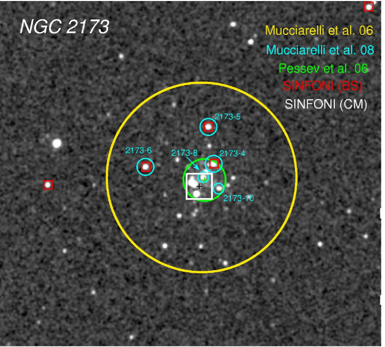
NGC 2173: Deciding about the cluster membership of the stars observed around this cluster was easier, due to the availability of high resolution spectroscopy of RGB stars in NGC 2173 from the study of Mucciarelli et al. (2008). As shown in Fig. 5, we have three stars outside of and one within the central SINFONI mosaic in common with their study. Based on high resolution spectra Mucciarelli et al. (2008) find that these four stars have very similar radial velocities (rms = 1.2 ) and negligible star-to-star scatter in the [Fe/H]. Thus we safely concluded that the first three stars outside of the SINFONI mosaic are cluster members and we included them in the final integrated spectrum for the cluster.
Column 7 in Table 3 lists the stars, which we added to the final spectra for each globular cluster.
4.3 Cluster light sampling
Our study shows that with a reasonable amount of mosaic tiles and no more than 1.5 hours VLT observing time, we can sample a significant fraction of the light from each of our sample of LMC GCs. We have seen that for well concentrated clusters there is no need for additional light sampling, other than a central mosaic, covering at least the half-light radius. The strategy of observing a mosaic on the cluster’s centre and then a sequence of the brightest and closest stars within a certain radius, works very well in the case of sparse and not luminous clusters, as well as for those, which are rich, but not well concentrated. However, there are still some doubts about the cluster membership of the brightest stars around the intermediate age clusters, especially in the case of carbon rich stars. For this reason we would need high resolution spectroscopy to measure their radial velocities and chemical composition and compare with other RGB stars.
Flux calibration of ground based spectroscopic data in the near-IR is particularly difficult, thus we cannot rely on direct luminosity estimates from our data. However, we can use the available photometry of Mucciarelli et al. (2006) to estimate the approximate amount of sampled light in the intermediate age clusters. In this study the authors provide not only integrated magnitudes and colours, but also estimates of the M- and C-type stars contributions to the total cluster light in the -band. From there we know that the -band light of NGC 2162 is dominated by only one carbon rich star, which is responsible for 60 % of the total cluster luminosity. This C-type star contributes with about 70 % to our final integrated cluster spectrum. From this we conclude that for this cluster we are missing only 10 % of the luminosity, measured by Mucciarelli et al. (2006). The situation with the other two intermediate age clusters is similar. NGC 1806 is quite rich in stars in comparison with the other two clusters, as seen in the -band images in Fig. 1. According to Mucciarelli et al. (2006) 22 % of the total cluster light is coming from stars with (AGB stars). About 77 % of it is due to four carbon stars. In our NGC 1806 integrated spectrum these four C-type stars account for 60 %. Following Mucciarelli et al. (2006), 15 % of the light in NGC 2173 are due to one C-type star. In our spectrum this star is responsible for 20 %. For the three old and metal poor clusters such detailed estimates of the contributions from different stellar phases are not available, thus we cannot make similar estimates for them as for the intermediate age clusters. Our central SINFONI mosaics cover more than one half-light radius. From this we conclude that the majority of the cluster light is covered.
According to these rough estimates it is evident that we have reached our goal set up in Sect. 1, namely to obtain representative luminosity weighted, integrated spectra in the -band for a group of clusters, having intermediate and old ages. The final spectra used for the scientific analysis in the following sections are shown in Fig. 6. The achieved signal-to-noise ratios are given in Table 5. The two clusters that have spectra dominated by carbon rich giants, NGC 1806 and NGC 2162, visually seem to have a significantly lower S/N than the other clusters. However, as mentioned already in Sect. 3.5, this does not reflect the reality: these spectra are dominated by numerous absorption lines from carbon-based molecules, which the method for computing S/N interprets as noise. To properly estimate the S/N one would need synthetic spectra, including the full spectral synthesis. This is clearly not possible, as we are aiming to provide first templates that could allow computation of such spectra. We estimated the S/N for these two clusters based on the amount of integrated flux as compared to the other clusters in our sample and assigned to them a conservative lower limit of S/N 80.

5 Line strength indices in the -band
The stellar population modelling technique allows us to obtain detailed estimates of the properties of integrated stellar populations by measuring, for example, the strengths of selected absorption or emission features in the spectra and comparing the measured values to the predicted ones. This approach has shown to be very effective in the optical wavelength range and a well established system, the so called Lick/IDS system (Faber et al. 1985; Worthey et al. 1994; Trager et al. 1998), is widely used. For the study of -band spectral features several index definitions have been adopted (e.g. Förster Schreiber 2000; Frogel et al. 2001; Silva et al. 2008; Mármol-Queraltó et al. 2008). To measure the line strengths of Na I and Ca I (see Fig. 6) we used the index definitions of Frogel et al. (2001), and for the strength of 12CO (2–0) the definitions of Mármol-Queraltó et al. (2008) and Maraston (2005).
The principle of measuring a near-IR index is the same as in the optical Lick system. The value is computed as the ratio of the flux in a central passband to the flux at the continuum level, measured in two pseudo-continuum passbands on both sides of the central passband. Due to the lack of a well defined continuum on the red side of the 12CO (2–0) feature, the index that Mármol-Queraltó et al. (2008) defined, uses two continuum passbands on the blue side. This index measure the ratio between the average fluxes in the continuum and the absorption bands. Maraston (2005) uses a CO index, which measures the ratio of the flux densities at 2.37 and 2.22 m, based on the HST/NICMOS filters F237M and F222M. The index is computed in units of magnitudes and is normalised to Vega. This index reflects the strength not only of 12CO (2–0), but also of the other CO absorption features in the range 2.3 – 2.4 m (see Fig. 6).
Prior to index measurements we broadened our spectra to a spectral resolution of 6.9 Å (FWHM) to match the resolution of similar earlier studies of the -band light of early type galaxies and stars obtained with VLT/ISAAC (Silva et al. 2008; Mármol-Queraltó et al. 2009). We measured the recession velocities of the LMC globular clusters and stars with the IRAF task fxcor and corrected for them. We did not apply velocity dispersion corrections to the indices due to the very low velocity dispersions of the clusters ( 10 , see previous section). The final index values are listed in Table 5.
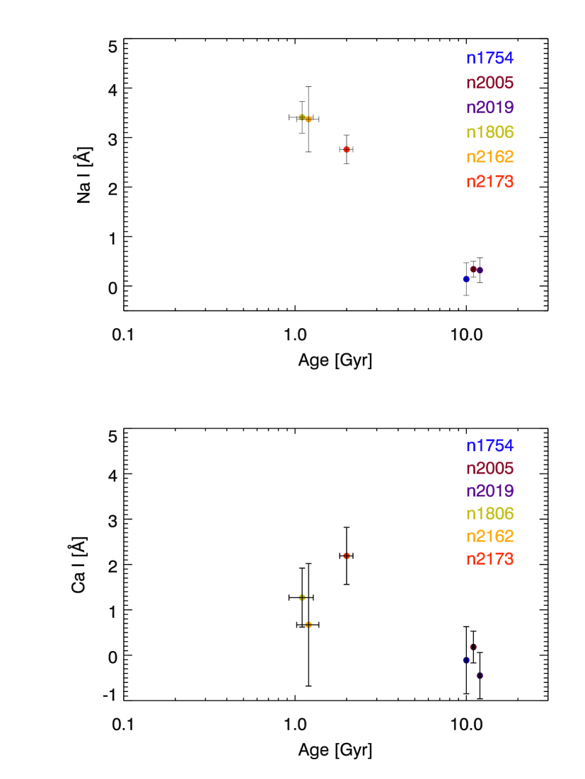
The current stellar population models, which include the near-IR wavelength range (e.g. Maraston 2005), have too low spectral resolution at these wavelengths ( 200 Å FWHM) to be able to give predictions for the weak and narrow features Na I and Ca I. Until more detailed models become available we can only empirically explore their dependance on the parameters of the globular clusters, derived from resolved light studies.
In Fig. 7 we show the dependance of the Na I and Ca I index on the age of the clusters. We see that the Na I index increases with decreasing age of the cluster and increasing metallicity. This result was already suggested by Silva et al. (2008), who find that the centres of early type galaxies in the Fornax cluster with signatures of a recent star formation, i.e. stronger H, have also stronger Na I indices. The Ca I index seems to show similar behaviour as (discussed further in the text) as function of age, albeit with larger error bars.
The 12CO (2–0) absorption feature at 2.29 m, which we described with the index, is much stronger and broader. Stellar population model predictions for its strength exist and will be discussed in the following section in more detail.
| Name | Na I [Å] | Ca I [Å] | CO [mag] | S/N | |
|---|---|---|---|---|---|
| (1) | (2) | (3) | (4) | (5) | (6) |
| NGC 1754 | 0.140.33 | -0.110.74 | 1.0820.005 | -0.0350.002 | 55 |
| NGC 2005 | 0.340.16 | 0.180.35 | 1.0860.003 | 0.0170.001 | 107 |
| NGC 2019 | 0.320.25 | -0.450.51 | 1.0680.003 | -0.0030.001 | 103 |
| NGC 1806 | 3.410.32 | 1.270.65 | 1.1290.005 | 0.0260.001 | 80 |
| NGC 2162 | 3.370.66 | 0.671.35 | 1.1080.010 | 0.0130.002 | 80 |
| NGC 2173 | 2.760.29 | 2.190.63 | 1.1860.005 | 0.1230.002 | 75 |
Notes: (1) Cluster name, (2) Na I index, (3) Ca I index, (4) index, (5) CO index, (6) signal-to-noise ratio of the integrated spectrum.
6 Comparisons with stellar population models
One of the goals of this project was to verify the predictions of the current stellar population models in the near-IR wavelength range. Such models are the ones presented in Maraston (2005). The author provides a full set of SEDs (spectral energy distributions) for different stellar populations with ages from 103 yr to 15 Gyr and covering a range of metallicities. These SEDs extend up to 2.5 m, but their spectral resolution in the near-IR wavelengths is rather low, with one pixel covering 100 .
The model predictions include the CO index, and for completeness we measured the index as defined by Mármol-Queraltó et al. (2008). In order to measure it for the models we had to interpolate the model SEDs linearly to a smaller wavelength step of 14 . We have chosen this value after a few tests to check the stability of the computation. Mármol-Queraltó et al. (2008) show that their index definition is very little dependent on instrumental or internal velocity broadening of the spectrum. However, the most extreme resolution they have tested is 70 (), while the resolution of the model SEDs is 200 (). We have measured the index in 10 stars from our sample with their nominal resolution and when broadened to match the resolution of the models. The broadened spectra have a index value, which is weaker by 0.04 with respect to the unbroadened spectra. An offset with this size is not going to influence our general conclusions about the integrated spectra of LMC GCs. This is further supported by the CO index values of the GCs, which exhibit the same relative values compared to the models. The CO index covers a very large wavelength range and is little dependent on the spectral resolution. Thus we decided to measure the index at the nominal resolution of our spectra (6.9 Å FWHM) and treat the model predictions with caution. Once higher resolution models become available, this comparison should be repeated in a more quantitative way. In the following subsection we discuss the comparison between the models and the data. For clarity we divided the globular clusters in two groups. In Sect. 6.1 we explore the three old and metal poor clusters NGC 1754, NGC 2005 and NGC 2019. In Sect. 6.2 we discuss the intermediate age globular clusters NGC 1806, NGC 2162 and NGC 2173.
6.1 Old clusters
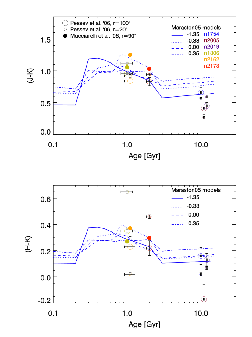
Literature data of the integrated near-IR colours of our sample of old and metal poor clusters are shown in Fig. 8 with open circles. The large open symbols represent the colours, derived from 100 radius aperture photometry, the small open symbols from 20 radius aperture photometry from Pessev et al. (2006). With blue lines we have overplotted SSP model predictions from Maraston (2005) for a Kroupa IMF and blue horizontal branch morphology. The metallicity which is closest to the one, derived for our GCs sample is denoted with a solid blue line, [Z/H] = –1.35. In the top panel the data agree reasonably well with the model colour. In the bottom panel the colours show a larger spread.
In Fig. 9 we show the comparison between model predictions and index measurements for 12CO (2–0). For the top panel we used the Maraston (2005) CO index, while for the bottom panel we used the index defined in Mármol-Queraltó et al. (2008). For stellar populations with an age of more than 3 Gyr the near-IR -band light is dominated by RGB stars, whose contribution stays approximately constant over large time scales. This is reflected in the stellar population models in Fig. 9, where the CO index remains almost constant at a given metallicity for ages 3 Gyr. Our observational data fit reasonably well with the model predictions, despite the slightly lower index values in the LMC GCs with respect to the [Z/H] = – 1.35 line. A possible reason for this, including the bluer colours of the globular clusters with respect to the models, may arise from the fact that the models use [Z/H] to describe the metallicity, which includes not only iron but also other heavy elements. The literature data, which we used, estimate the metallicity only based on [Fe/H]. If the globular clusters in our sample follow similar chemical trends as the old LMC globular clusters discussed in Mucciarelli et al. (2009) we might expect a better agreement.
6.2 Intermediate age clusters
We divided the intermediate age GCs sample into two sub-samples, according to the SWB type of the clusters. NGC 1806 and NGC 2162 have SWB type V and thus their age is estimated to be around 1.1 Gyr (Frogel et al. 1990). NGC 2173 has SWB between V and VI and an age of approximately 2 Gyr (Frogel et al. 1990). Based on colour-magnitude diagram methods different authors give slightly higher or lower ages for these clusters. In order to be consistent with the age calibration of the SSP models presented by Maraston (2005) we have decided to use the ages based on SWB types, as was done in these models.
In Fig. 8, a compilation of literature photometric data for the intermediate age GCs in our sample are shown. According to their mean metallicity the closest model is shown with the dotted lines and has [Z/H] = – 0.33. The integrated near-IR colours within an aperture with radius of 90 from Mucciarelli et al. (2006) are shown with solid circles. The photometry of Pessev et al. (2006) with different aperture sizes is shown with open circles.
Comparing the large filled and open symbols in Fig. 8, we see evidence for disagreement between the two studies, despite the fact that Mucciarelli et al. (2006) do not provide error bars. We also see that according to the different apertures of Pessev et al. (2006) the intermediate age clusters exhibit colour gradients of about 0.2m in and . However, not always in the same direction. In the clusters become systematically bluer with increasing radius, while in NGC 2162 gets redder. In general colour gradients in globular clusters can be explained by mass segregation, which makes the most massive, and thus the most evolved, stars to be concentrated towards the centre. However, this effect is not expected to be that large, in comparison with the values that Pessev et al. (2006) report. The -band magnitudes of Pessev et al. (2006) are fainter by approximately one magnitude as compared to the ones measured by Mucciarelli et al. (2006) for NGC 1806 and NGC 2162 for a similar aperture and the colours are bluer. These effects could be either due to an overestimated LMC field decontamination, if Pessev et al. (2006) removed the reddest stars, or underestimation of the field in the case of Mucciarelli et al. (2006). We can check this hypothesis using NGC 2162, where the -band light of the globular cluster is dominated by one single carbon rich star. By adding its -band magnitude, taken from the 2MASS catalogue, to the integrated (over 100″) magnitude of the cluster, taken from Pessev et al. (2006), we obtain a final -band magnitude in much better agreement with Mucciarelli et al. (2006). Field carbon stars are not observed frequently at the location of this cluster in the LMC, thus there is a high probability that this star is a cluster member. Therefore the large colour gradients present in the work of Pessev et al. (2006) and their fainter -band magnitudes are most probably due to their oversubtraction of the LMC field star contribution for these two clusters.
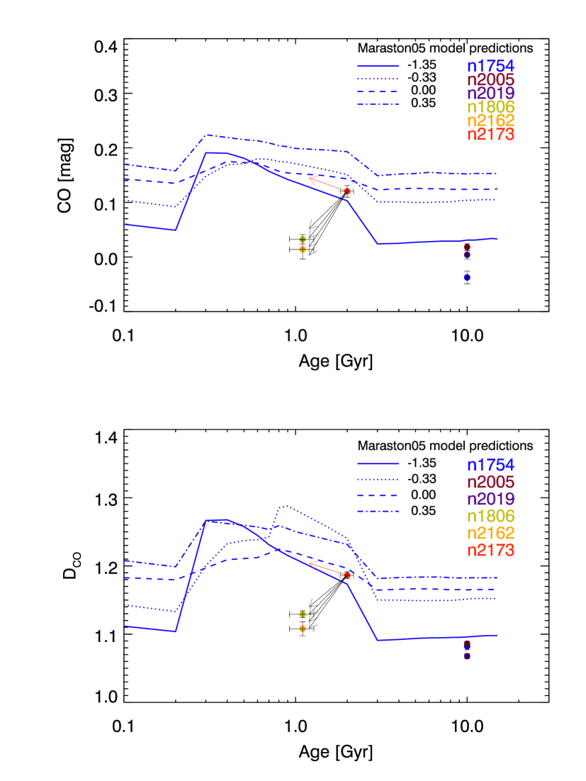
Our comparison of the SSP model predictions with the observed CO indices of LMC globular clusters is shown in Fig. 9. For the intermediate age clusters on both panels the closest model metallicity to the data is denoted with the dotted line, [Z/H]= – 0.33. NGC 2173 (age 2 Gyr) is marked with a red filled circle and agrees reasonably well with the model predictions. However, the other two intermediate age clusters, NGC 1806 (light green filled circle) and NGC 2162 (orange filled circle) have CO index values much lower than the model predictions, independent from the CO index definition.
6.2.1 Cluster light sampling and stochastic effects
We have tested a few scenarios, which can provide possible explanations of the observed trends. The first scenario, which we have investigated is whether we are sampling well the total cluster light. We consider this is not a problem following the estimations about the sampled cluster light during our observations, made in Sect. 4.3. The second question is, are the two clusters stochastically sampling the IMF well? Here the answer is ”most likely”. Lançon & Mouhcine (2000) show that the CO index is significantly influenced by stochastic fluctuations for intermediate age stellar populations with , but when the mass reaches and above the fluctuations are much less prominent. Our intermediate age globular clusters have masses closer to the range (e.g. NGC 2162, McLaughlin & van der Marel 2005) and thus are not expected to exhibit large variations in the CO index. By building a super cluster from NGC 1806 and NGC 2162 we are reducing the stochastic effects further, and we still find the same behaviour of decreasing index value. However, this finding needs to be further verified with larger samples of intermediate age clusters.
6.2.2 Different Carbon stars in LMC and Milky Way?
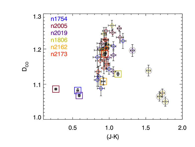
The careful investigation of the integrated spectra of LMC intermediate age GCs showed us that the presence of C-type stars does not only influence the overall colours of the clusters, as discussed above, but also their CO index. Fig. 10, where we plotted the index as a function of the colour for all of the objects in our observational sample, shows a general trend of increasing 12CO (2–0) index with the colour becoming redder. This is typical for oxygen rich (or M-type) stars (e.g. Frogel et al. 1990). However, stars with 1.3 show a decreasing 12CO (2–0) line strength. These are exactly the carbon rich stars, separated in Fig. 2 with a slanted line, and denoted in Fig. 10 with circles. Similar trends for carbon stars of LMC globular clusters have been observed by Frogel et al. (1990).
According to Frogel et al. (1990) the clusters, which harbour the brightest carbon stars are of SWB type V and VI. For these clusters, carbon stars contribute about 40 % of the total bolometric light and this observation is taken into count in the calibrations of the computed SEDs of Maraston (2005) models. Using the spectrum of NGC 2173, which is very convenient for this kind of tests, because it is the one with a minimal carbon star contribution in our sample, we checked what is the effect of different ratios of M-type to C-type stars on the CO line strength of the final integrated spectrum. The results are shown in Fig. 9 with black arrows, which start from the initial position of NGC 2173 (red filled circle) and end at the age of clusters with SWB type V, i.e. 1.1 Gyr. The reason for this age scaling is that a larger carbon star contribution would mimic the spectrum of a younger cluster. The arrows show, from top to bottom, an increasing fraction of carbon star contribution to the final cluster light – 40 %, 50 %, 60 % and 70 %, respectively originate from the C-type star. The same is valid for both the CO index used by Maraston (2005) and the index defined by Mármol-Queraltó et al. (2008). This simple experiment shows us that we are able to reproduce the lower observed CO index values in the integrated spectra of LMC globular clusters having SWB type V with an increasing fraction of the carbon star contribution. The same kind of tests, but performed with integrated colours, make the cluster redder, as expected when having an increased fraction of carbon rich stars.
The models of Maraston (2005) include a careful treatment of the TP-AGB stellar phase, which is of great importance for stellar populations with ages between 0.3 and 2 Gyr, due to its very high luminosity. The empirical photometric calibration of the models has been done with the near-IR photometric data of LMC globular clusters and AGB stars of Persson et al. (1983) and Frogel et al. (1990). Spectra of carbon-rich stars are also included. They come from the database of Lançon & Mouhcine (2002), which contains averaged C-type star spectra. These authors have obtained 21 spectra of carbon-rich luminous pulsating variable stars in the Milky Way. However, due to the small temperature scales of the sample, they do not consider as justified to have more than a few averaged bins. The carbon stars have been grouped according to their temperature, defined by their colour. The first three bins contain averages of 6 C-type star spectra each. Bins 4 and 5 contain the spectra of a single very red star, R Lep, near maximum and minimum light. The temperature of the stars is decreasing with increasing bin number.
If carbon rich stars in the Galaxy and the LMC have different CO absorption strengths, then this would have a profound impact on the model predictions. Differences in the CO index have been observed by e.g. Frogel et al. (1990) using narrow-band filters, where they compare the CO value of LMC clusters C-type stars and their counterparts in the Milky Way. The LMC stars have systematically weaker CO indices at a given colour. In Fig. 11 we show the CO index values as a function of colour, measured in C-type stars belonging to our sample (filled symbols), compared to the CO index that we measured on the averaged spectra of Lançon & Mouhcine (2002). The least-squares linear fit to the LMC carbon rich stars is shown as a solid line:
| (2) |
| (3) |
The Milky Way averaged spectra are marked with open symbols, with a bin number assigned to each. The dashed line is showing the linear least-squares fit to the averaged spectra:
| (4) |
| (5) |
From this figure we see that the trends for C-type stars in the Milky Way and the LMC generally disagree. Moreover, stars with have increasingly different CO index values, which explains why our LMC GCs sample fits the model predictions for integrated colours, but not for the CO index.
We made another test of including carbon star light to the spectrum of NGC 2173, but this time using the spectrum of bin 3 of Lançon & Mouhcine (2002). The result is shown in Fig. 9 with a red arrow. For this case specifically the ratio of carbon star to the original spectrum was 6:4. Different ratios, as in the previous test, gave similar values. We see that the resultant CO index value increases by adding Milky Way carbon stars and follows the trends predicted by the models, while the inclusion of LMC cluster carbon stars leads to a decrease of the index. We find this as an attractive explanation for the discrepancy between the models and the data.

At this point the question arises why C-type stars in the LMC and the Galaxy have different CO line strengths at a given near-IR colour? We have to treat this issue with care, since not all of the carbon stars in the Lançon & Mouhcine (2002) library disagree with the relation for the LMC C-stars. The averaged spectrum from bin 2 agrees with the LMC relation. In the bottom panel of Fig. 11 we indicated with an asterisk another C-type star from the Milky Way, located in the Galactic open cluster NGC 2477 ([Fe/H]= – 0.02, (Houdashelt et al. 1992). A -band spectrum of this star has been published in Silva et al. (2008), however the authors did not discuss its properties. Its colour and index value are consistent with the relation for LMC C-type stars, given in Equation 2.
AGB stars in populations with lower metallicity are more likely to become C-type. A star becomes C-type when the ratio of carbon to oxygen atoms in its atmosphere becomes larger than one. Then all the oxygen is locked up in CO molecules, and there is still some extra carbon in the atmosphere. For the metal-poor stars there is less oxygen in the atmosphere in the first place. Therefore these stars need to dredge up less carbon in order to overcome, in relative amount, the quantity of oxygen and so become C-type. The remaining carbon is used to form other molecules, like C2, CN and CH. In this way the CO index as we measure it decreases. Note that the overall line strength of the 12CO (2–0) may not decrease significantly. For example see Fig. 6, where the 12CO (2–0) features in NGC 1806 and NGC 2162 do not seem to be much weaker, than in NGC 2173. But the CO indices, which we use to describe the behaviour of this feature, take into account the continuum shape as well, which in the case of carbon stars is severely affected by the presence of features like C2, CN or CH. In more metal rich stars the amount of oxygen atoms is higher and all of the available carbon is used to form CO molecules, which makes a stronger CO index in oxygen-rich stars. The different CO indices in Milky Way and LMC carbon-rich stars are due to a real change in the depth of the CO absorption features.
The observed difference between the Lançon & Mouhcine (2002) library carbon stars in the Milky Way and the ones in our sample in the LMC has important implications on the stellar populations models. The photometric calibration of the intermediate age populations in the models of Maraston (2005) has been performed with globular clusters in the LMC. However, for the spectral calibration, spectra of carbon-rich stars in the Milky Way have been used, which leads to inconsistent results. There might be a number of reasons for the observed inconsistencies, like different metallicities of the carbon stars or the phase of the pulsation in which they were observed. Our results clearly show the necessity of a better understanding of the properties of carbon rich stars and the need of larger empirical stellar libraries to improve model predictions.
7 Conclusions
The goal of this project is to provide an empirical spectral library in the near-IR for integrated stellar populations with ages 1 Gyr, which will be used to test the current and calibrate the future stellar population models. In this paper we have presented the first results from a pilot study of the -band spectroscopic properties of a sample of six globular clusters in the LMC. To validate the observational strategy, data reduction and analysis methods, we have selected from the catalogue of Bica et al. (1999) three out of 38 GCs with SWB type VII to represent the old (10 Gyr) and metal poor ([Fe/H]–1.4) population of the LMC, and three out of 71 clusters with SWB types V and VI to explore the properties of the intermediate age (1 – 3 Gyr) and more metal rich ([Fe/H]–0.4) component of the population. For each cluster our integrated spectroscopy covers the central and in most of the cases we have sampled about half the light. However, in order to better sample bright AGB stars, which are the most important contributors to the integrated cluster light in the near-IR, we have observed up to 9 of the brightest stars outside the central mosaics, but still within the tidal radii of the clusters, that have near-IR colours and magnitudes consistent with bright red giants in the observed clusters. We obtained integrated luminosity weighted spectra for the six clusters, measured the line strengths of Na I, Ca I and 12CO (2–0) absorption features in the -band and compared the strength of 12CO (2–0) with the stellar population models of Maraston (2005).
The observing strategy to cover at least the central half-light radius with a number of SINFONI pointings showed to be an efficient way in sampling the near-IR light of old ( 10 Gyr) clusters. For the intermediate age and sparse clusters, which are dominated by just a few very bright stars, observing a central mosaic plus a number of the brightest stars in the vicinity of the cluster is a better choice for optimal cluster light sampling. The availability of high spectral resolution spectroscopy greatly helps the differentiation of the cluster member stars from the LMC field population.
In intermediate age clusters the largest amount of light originates from oxygen (M-type) and carbon-rich (C-type) AGB stars. Different ratios of the contributions by these two types of stars can lead to significant changes in the near-IR 12CO (2–0) line strength. According to our observations, when the C-type stars contribution peaks (at 1 Gyr) the observed CO line strength is weak and then increases fast to reach its maximum for clusters with age 2 Gyr. It is important to note that a weak line strength of 12CO (2–0) does not mean that there is less CO in these clusters/stars. The indices, which are used to describe the line strengths, take also into account the continuum shape, which in the case of carbon-rich stars is severely affected by typical for this type of stars absorption features and thus the resultant index value is low.
The comparison of our data with the stellar population models of Maraston (2005), in terms of CO line strength, shows a disagreement for the youngest clusters in our sample. For clusters with age 1 Gyr the models predict maximal CO line strength, while we observe the opposite: the CO strength is significantly weaker. At the same time, literature data of the integrated colours of the clusters are consistent with these models. We explain these discrepancies as due to the different origin of the C-type stars used to calibrate the models and the ones in our data sample. The stars, used for model calibration, are Milky Way carbon stars, while our carbon stars are born in the LMC. We support this scenario with Fig. 11, where we show that carbon rich stars in the Milky Way and LMC, which have similar colour, have very different CO line strengths. This deserves further investigation and hopefully the next generation of carbon star models (e.g. Aringer et al. 2009) will help us to elucidate whether a systematic effect of the metallicity on CO indices is expected, or the found discrepancy is due to the small sample of individual observations of variable stars in existing libraries.
The near-IR Na I index shows a dependance on the age of the clusters – it is decreasing with an increasing age. The combination between optical and near-IR spectral indices seems to offer possibilities to break the age-metallicity degeneracy, but more accurate and detailed stellar population models are necessary in the near-IR wavelength range.
These models are of paramount importance, when studying the spatially resolved stellar populations of nearby galaxies. Adaptive optics assisted observations allow for the best correction of the Earth’s atmosphere perturbing effects when observing in the near-IR. First attempts to explore galaxy evolution via spatially resolved near-IR spectroscopy (e.g. Lyubenova et al. 2008; Davidge et al. 2008; Nowak et al. 2008) have shown the need for a better understanding of the properties of stellar populations in this wavelength range. The availability of detailed and reliable stellar population models in the near-IR will open up a new window to the exploration of galaxy formation and evolution.
The final integrated spectra of the six LMC globular clusters will be made available via the Strasbourg astronomical Data Center (CDS).
Acknowledgements.
We are grateful to many ESO staff astronomers who took the data presented in this paper in service mode operations at La Silla Paranal Observatory. We would like to thank Maria-Rosa Cioni, Claudia Maraston, and Daniel Thomas for helpful discussions. Finally, we thank the anonymous referee for her/his helpful suggestions.References
- Alves (2004) Alves, D. R. 2004, New Astronomy Review, 48, 659
- Alves et al. (2002) Alves, D. R., Rejkuba, M., Minniti, D., & Cook, K. H. 2002, ApJ, 573, L51
- Aringer et al. (2009) Aringer, B., Girardi, L., Nowotny, W., Marigo, P., & Lederer, M. T. 2009, A&A, 503, 913
- Beasley et al. (2002) Beasley, M. A., Hoyle, F., & Sharples, R. M. 2002, MNRAS, 336, 168
- Bernardi et al. (2005) Bernardi, M., Sheth, R. K., Nichol, R. C., Schneider, D. P., & Brinkmann, J. 2005, AJ, 129, 61
- Bessell & Brett (1988) Bessell, M. S. & Brett, J. M. 1988, PASP, 100, 1134
- Bica et al. (1996) Bica, E., Claria, J. J., Dottori, H., Santos, Jr., J. F. C., & Piatti, A. E. 1996, ApJS, 102, 57
- Bica et al. (1999) Bica, E. L. D., Schmitt, H. R., Dutra, C. M., & Oliveira, H. L. 1999, AJ, 117, 238
- Blanco & McCarthy (1983) Blanco, V. M. & McCarthy, M. F. 1983, AJ, 88, 1442
- Bonnet et al. (2004) Bonnet, H., Abuter, R., Baker, A., et al. 2004, in The ESO Messenger, Vol. 117
- Borissova et al. (2004) Borissova, J., Minniti, D., Rejkuba, M., et al. 2004, A&A, 423, 97
- Bruzual & Charlot (1993) Bruzual, A. G. & Charlot, S. 1993, ApJ, 405, 538
- Bruzual & Charlot (2003) Bruzual, G. & Charlot, S. 2003, MNRAS, 344, 1000
- Cappellari et al. (2006) Cappellari, M., Bacon, R., Bureau, M., et al. 2006, MNRAS, 366, 1126
- Cioni et al. (2006) Cioni, M.-R. L., Girardi, L., Marigo, P., & Habing, H. J. 2006, A&A, 448, 77
- Cox (2000) Cox, A. N. 2000, Allen’s astrophysical quantities, ed. A. N. Cox
- Da Costa (1991) Da Costa, G. S. 1991, in IAU Symposium, Vol. 148, The Magellanic Clouds, ed. R. Haynes & D. Milne, 183
- Davidge et al. (2008) Davidge, T. J., Beck, T. L., & McGregor, P. J. 2008, ApJ, 677, 238
- Dirsch et al. (2000) Dirsch, B., Richtler, T., Gieren, W. P., & Hilker, M. 2000, A&A, 360, 133
- Dubath et al. (1997) Dubath, P., Meylan, G., & Mayor, M. 1997, A&A, 324, 505
- Eisenhauer et al. (2003) Eisenhauer, F., Abuter, R., Bickert, K., et al. 2003, in Proceedings of the SPIE, ed. M. Iye & A. F. M. Moorwood
- Faber et al. (1985) Faber, S. M., Friel, E. D., Burstein, D., & Gaskell, C. M. 1985, ApJS, 57, 711
- Ferraro et al. (2004) Ferraro, F. R., Origlia, L., Testa, V., & Maraston, C. 2004, ApJ, 608, 772
- Fioc & Rocca-Volmerange (1997) Fioc, M. & Rocca-Volmerange, B. 1997, A&A, 326, 950
- Förster Schreiber (2000) Förster Schreiber, N. M. 2000, AJ, 120, 2089
- Frogel et al. (1990) Frogel, J. A., Mould, J., & Blanco, V. M. 1990, ApJ, 352, 96
- Frogel et al. (1978) Frogel, J. A., Persson, S. E., Matthews, K., & Aaronson, M. 1978, ApJ, 220, 75
- Frogel et al. (2001) Frogel, J. A., Stephens, A., Ramírez, S., & DePoy, D. L. 2001, AJ, 122, 1896
- Grocholski et al. (2006) Grocholski, A. J., Cole, A. A., Sarajedini, A., Geisler, D., & Smith, V. V. 2006, AJ, 132, 1630
- Houdashelt et al. (1992) Houdashelt, M. L., Frogel, J. A., & Cohen, J. G. 1992, AJ, 103, 163
- Johnson et al. (2006) Johnson, J. A., Ivans, I. I., & Stetson, P. B. 2006, ApJ, 640, 801
- Kodama & Arimoto (1997) Kodama, T. & Arimoto, N. 1997, A&A, 320, 41
- Kuntschner (2000) Kuntschner, H. 2000, MNRAS, 315, 184
- Lançon & Mouhcine (2000) Lançon, A. & Mouhcine, M. 2000, in Astronomical Society of the Pacific Conference Series, Vol. 211, Massive Stellar Clusters, ed. A. Lançon & C. M. Boily, 34
- Lançon & Mouhcine (2002) Lançon, A. & Mouhcine, M. 2002, A&A, 393, 167
- Leitherer et al. (1999) Leitherer, C., Schaerer, D., Goldader, J. D., et al. 1999, ApJS, 123, 3
- Lyubenova (2009) Lyubenova, M. 2009, PhD thesis, Ludwig-Maximilians-Universität, Munich, available from the author
- Lyubenova et al. (2008) Lyubenova, M., Kuntschner, H., & Silva, D. R. 2008, A&A, 485, 425
- Mackey et al. (2008) Mackey, A. D., Broby Nielsen, P., Ferguson, A. M. N., & Richardson, J. C. 2008, ApJ, 681, L17
- Mackey & Gilmore (2003) Mackey, A. D. & Gilmore, G. F. 2003, MNRAS, 338, 85
- Maraston (1998) Maraston, C. 1998, MNRAS, 300, 872
- Maraston (2005) Maraston, C. 2005, MNRAS, 362, 799
- Mármol-Queraltó et al. (2008) Mármol-Queraltó, E., Cardiel, N., Cenarro, A. J., et al. 2008, A&A, 489, 885
- Mármol-Queraltó et al. (2009) Mármol-Queraltó, E., Cardiel, N., Sánchez-Blázquez, P., et al. 2009, ArXiv e-prints 0909.5385
- McLaughlin & van der Marel (2005) McLaughlin, D. E. & van der Marel, R. P. 2005, ApJS, 161, 304
- Mucciarelli et al. (2008) Mucciarelli, A., Carretta, E., Origlia, L., & Ferraro, F. R. 2008, AJ, 136, 375
- Mucciarelli et al. (2006) Mucciarelli, A., Origlia, L., Ferraro, F. R., Maraston, C., & Testa, V. 2006, ApJ, 646, 939
- Mucciarelli et al. (2009) Mucciarelli, A., Origlia, L., Ferraro, F. R., & Pancino, E. 2009, ApJ, 695, L134
- Nowak et al. (2008) Nowak, N., Saglia, R. P., Thomas, J., et al. 2008, MNRAS, 391, 1629
- Olsen et al. (1998) Olsen, K. A. G., Hodge, P. W., Mateo, M., et al. 1998, MNRAS, 300, 665
- Olszewski et al. (1991) Olszewski, E. W., Schommer, R. A., Suntzeff, N. B., & Harris, H. C. 1991, AJ, 101, 515
- Persson et al. (1983) Persson, S. E., Aaronson, M., Cohen, J. G., Frogel, J. A., & Matthews, K. 1983, ApJ, 266, 105
- Pessev et al. (2006) Pessev, P. M., Goudfrooij, P., Puzia, T. H., & Chandar, R. 2006, AJ, 132, 781
- Renzini (1998) Renzini, A. 1998, AJ, 115, 2459
- Sánchez-Blázquez et al. (2007) Sánchez-Blázquez, P., Forbes, D. A., Strader, J., Brodie, J., & Proctor, R. 2007, MNRAS, 377, 759
- Sánchez-Blázquez et al. (2009) Sánchez-Blázquez, P., Jablonka, P., Noll, S., et al. 2009, A&A, 499, 47
- Santos & Frogel (1997) Santos, Jr., J. F. C. & Frogel, J. A. 1997, ApJ, 479, 764
- Schiavon (2007) Schiavon, R. P. 2007, ApJS, 171, 146
- Searle et al. (1980) Searle, L., Wilkinson, A., & Bagnuolo, W. G. 1980, ApJ, 239, 803
- Silva et al. (2008) Silva, D. R., Kuntschner, H., & Lyubenova, M. 2008, ApJ, 674, 194
- Skrutskie et al. (2006) Skrutskie, M. F., Cutri, R. M., Stiening, R., et al. 2006, AJ, 131, 1163
- Stoehr et al. (2007) Stoehr, F., Fraquelli, D., Kamp, I., et al. 2007, Space Telescope European Coordinating Facility Newsletter, Volume 42, p.4, 42, 4
- Thomas et al. (2003) Thomas, D., Maraston, C., & Bender, R. 2003, MNRAS, 339, 897
- Thomas et al. (2005) Thomas, D., Maraston, C., Bender, R., & Mendes de Oliveira, C. 2005, ApJ, 621, 673
- Tinsley (1980) Tinsley, B. M. 1980, Fundamentals of Cosmic Physics, 5, 287
- Trager et al. (2000) Trager, S. C., Faber, S. M., Worthey, G., & González, J. J. 2000, AJ, 119, 1645
- Trager et al. (1998) Trager, S. C., Worthey, G., Faber, S. M., Burstein, D., & Gonzalez, J. J. 1998, ApJS, 116, 1
- van den Bergh (1998) van den Bergh, S. 1998, PASP, 110, 1377
- Vazdekis et al. (1996) Vazdekis, A., Casuso, E., Peletier, R. F., & Beckman, J. E. 1996, ApJS, 106, 307
- Worthey (1994) Worthey, G. 1994, ApJS, 95, 107
- Worthey et al. (1994) Worthey, G., Faber, S. M., Gonzalez, J. J., & Burstein, D. 1994, ApJS, 94, 687
- Zaritsky et al. (1997) Zaritsky, D., Harris, J., & Thompson, I. 1997, AJ, 114, 1002