Radiative Transfer Modeling of Lyman Alpha Emitters. I. Statistics of Spectra and Luminosity

Abstract

We combine a cosmological reionization simulation with box size of 100$h^{-1}{\rm Mpc}$ on a side and a Monte Carlo Ly$\alpha$ radiative transfer code to model Lyman Alpha Emitters (LAEs) at $z\sim$5.7. The model introduces Ly$\alpha$ radiative transfer as the single factor for transforming the intrinsic Ly$\alpha$ emission properties into the observed ones. Spatial diffusion of Ly$\alpha$ photons from radiative transfer results in extended Ly$\alpha$ emission and only the central part with high surface brightness can be observed. Because of radiative transfer, the appearance of LAEs depends on density and velocity structures in circumgalactic and intergalactic media as well as the viewing angle, which leads to a broad distribution of apparent (observed) Ly$\alpha$ luminosity for a given intrinsic Ly$\alpha$ luminosity. Radiative transfer also causes frequency diffusion of Ly$\alpha$ photons. The resultant Ly$\alpha$ line is asymmetric with a red tail. The peak of the Ly$\alpha$ line shifts towards longer wavelength and the shift is anti-correlated with the apparent to intrinsic Ly$\alpha$ luminosity ratio. The simple radiative transfer model provides a new framework for studying LAEs. It is able to explain an array of observed properties of $z\sim$5.7 LAEs in Ouchi et al. (2008), producing Ly$\alpha$ spectra, morphology, and apparent Ly$\alpha$ luminosity function (LF) similar to those seen in observation. The broad distribution of apparent Ly$\alpha$ luminosity at fixed UV luminosity provides a natural explanation for the observed UV LF, especially the turnover towards the low luminosity end. The model also reproduces the observed distribution of Ly$\alpha$ equivalent width (EW) and explains the deficit of UV bright, high EW sources. Because of the broad distribution of the apparent to intrinsic Ly$\alpha$ luminosity ratio, the model predicts effective duty cycles and Ly$\alpha$ escape fractions for LAEs.

1. Introduction

More than four decades ago, Partridge & Peebles (1967) proposed that prominent Ly$\alpha$ emission reprocessed from ionizing photons of young stars in galaxies can be used to detect high-redshift galaxies. The first successful detections of high-redshift Ly$\alpha$ emitting galaxies, or Ly$\alpha$ emitters (LAEs), were made $\sim$ 30 years later (e.g., Hu & McMahon, 1996; Cowie & Hu, 1998; Dey et al., 1998; Hu et al., 1998, 1999). Recently, important advances have been made on the observational front to detect LAEs at $z\gtrsim 6$ (e.g., Hu et al., 1998, 2002, 2004, 2005, 2006; Rhoads et al., 2003; Malhotra & Rhoads, 2004; Horton et al., 2004; Stern et al., 2005; Kashikawa et al., 2006; Shimasaku et al., 2006; Iye et al., 2006; Cuby et al., 2007; Ouchi et al., 2007, 2008; Stark et al., 2007a; Nilsson et al., 2007; Willis et al., 2008; Ota et al., 2008).

LAEs can be efficiently detected through narrow-band imaging or with integral-field-units (IFU) spectroscopy. Owing to the high efficiency of target detection, LAEs naturally become objects for large surveys of high-redshift galaxies. Besides providing clues to the formation and evolution of galaxies at the time when the universe was still young, LAEs are an important tracer of the large-scale structure. The clustering of LAEs may be used to constrain cosmological parameters. In particular, the large-volume surveys such as the Hobby-Eberly Telescope Dark Energy Experiment (HETDEX; Hill et al. 2008) will enable the detection of the baryon acoustic oscillations (BAO) features (e.g., Eisenstein et al., 2005) in the LAE power spectrum. The BAO and the shape of the power spectrum can be used to measure the expansion history of the universe at early epochs ($z\sim 3$), which constrains the evolution of dark energy and the curvature of the universe.

LAEs are also a key probe of the high-redshift intergalactic medium (IGM), especially across the reionization epoch. The use of LAEs to learn about reionization has been the subject of intense study (e.g., Miralda-Escudé & Rees, 1998; Miralda-Escudé, 1998; Haiman & Spaans, 1999; Santos, 2004; Haiman & Cen, 2005; Dijkstra et al., 2007; Wyithe & Cen, 2007). Suitably devised statistics, including luminosity function (LF) and correlation functions of LAEs, can be used to constrain the neutral fraction of the IGM during reionization (Malhotra & Rhoads, 2004; Haiman & Cen, 2005; Kashikawa et al., 2006; Furlanetto et al., 2006; Dijkstra et al., 2007; McQuinn et al., 2007; Mesinger & Furlanetto, 2008; Iliev et al., 2008; Dayal et al., 2008, 2009). By comparing the LFs of $z\sim 5.7$ and $z\sim 6.5$ LAEs, Malhotra & Rhoads (2004) conclude that reionization was largely complete at $z\sim 6.5$ (also see Dijkstra et al. 2007). McQuinn et al. (2007) show that, with the angular correlation function of the 58 available $z\sim 6.6$ LAEs in the Subaru Deep Field (Kashikawa et al., 2006), limits may be placed on the IGM neutral fraction, favoring a fully ionized universe at $z\sim 6.6$.

However, none of the previous work of LAEs mentioned above used reionization simulations with concurrent treatment of hydrodynamics plus radiative transfer of ionizing photons and Ly$\alpha$ photons. Hydrodynamic and radiative transfer simulations provide realistic neutral gas distributions, and Ly$\alpha$ radiative transfer yields detailed properties of the Ly$\alpha$ emission. Realistic Ly$\alpha$ radiative transfer calculations have been applied to high-redshift LAEs in cosmological simulations (e.g., Tasitsiomi, 2006). The application, however, is limited to a few individual sources, which do not form a sample for statistical study.

McQuinn et al. (2007) and Iliev et al. (2008) studied a sample of LAEs in reionization simulations with cosmological volume. However, the radiative transfer of Ly$\alpha$ photons is treated in a simplistic way in their study: the observed Ly$\alpha$ spectrum is modeled as the intrinsic line profile modified by $\exp(-\tau_{\nu})$, where $\tau_{\nu}$ is the optical depth at frequency $\nu$ along the line of sight. Although this $\exp(-\tau_{\nu})$ model can yield insights into the properties of the observed Ly$\alpha$ emission, such as the effect of IGM on the observability of LAEs, it is far from a complete description of the radiative transfer of Ly$\alpha$ photons. First, during the propagation, Ly$\alpha$ photons experience frequency diffusion, which is neglected by the simple $\exp(-\tau_{\nu})$ model. The $\exp(-\tau_{\nu})$ model removes Ly$\alpha$ photons at a given frequency according to the Ly$\alpha$ optical depth, and no frequency change occurs for any Ly$\alpha$ photon, therefore it does not yield correct Ly$\alpha$ spectra. Second, the simple $\exp(-\tau_{\nu})$ model does not account for the spatial diffusion of Ly$\alpha$ photons either. LAEs in this model appear as point sources in Ly$\alpha$ and there is no surface brightness information. Even if Ly$\alpha$ photons start from a point source, spatial diffusion due to radiative transfer would lead to an extended source. Observationally, LAEs indeed appear to be extended and they are defined by a surface brightness threshold in the narrow-band image (e.g., Ouchi et al., 2008). Therefore, although the simple $\exp(-\tau_{\nu})$ model may provide useful insight, it likely falls short for predicting the detailed properties of the observed Ly$\alpha$ emission from LAEs.

To correctly understand high-redshift LAEs and use them for cosmological study, a full calculation of radiative transfer of Ly$\alpha$ photons for a large sample of LAEs in cosmological reionization simulation is necessary, as will be evident later. In this work, we aim to perform detailed radiative transfer calculation of Ly$\alpha$ photons (Zheng & Miralda-Escudé, 2002) from LAEs in a self-consistent fashion through radiation-hydrodynamic reionization simulations (Trac et al., 2008). For this paper, we focus on studying statistical properties of $z\sim 5.7$ LAEs and show how the radiative transfer calculation aids our understanding of the observed properties of LAEs. The clustering properties of LAEs from this study will be presented in another paper (Paper II; Zheng et al. in prep.). The paper is organized as follows. In § 2 we review the cosmological reionization simulation used in this work and in § 3 we describe the Ly$\alpha$ radiative transfer calculation. In § 4, we study in details the Ly$\alpha$ emission from an individual source chosen from the simulation box to gain a general view of the effect of Ly$\alpha$ radiative transfer on the appearance of LAEs. Then, we present the statistical properties of LAEs in § 5, including their spectra and luminosity, from our modeling of an ensemble of sources in the simulation box. We compare our modeling results with observations for $z\sim 5.7$ LAEs and discuss the implications in our understanding of LAEs. § 7 is devoted to identifying important physical factors in shaping the observed Ly$\alpha$ emission of LAEs. We summarize and discuss the results in § 8.

2. Radiation Hydrodynamic Simulation of Cosmological Reionization

In this work, we perform a Ly$\alpha$ radiative transfer calculation to model LAEs. The sources and physical properties of gas are taken from the outputs of a cosmological reionization simulation.

The cosmological simulation (Trac et al., 2008) models cosmic reionization by using a hybrid approach to solve the coupled evolution of the dark matter, baryons, and radiation (Trac & Pen 2004, 2006; Trac & Cen 2007). First, a high-resolution $N$-body simulation was run, with 3072³ dark matter particles on a mesh of 11,520³ cells in a box of 100$h^{-1}{\rm Mpc}$ (comoving) on a side, and collapsed dark matter halos were identified on the fly. These halos are the sites to form sources of ionizing photons. The high resolution and large box size of the simulation make it possible to resolve small scale structures and to reduce sample variance for source statistics.

Hydrodynamics and radiative transfer of ionizing photons are simulated with moderate resolution (equal numbers, 1536³, of dark matter particles, gas cells, and adaptive rays). Within the limits of available computational resources, the multi-grid approach adopted in the simulation maximizes the resolution of the individual numerical components (gas and radiation) in order to model the corresponding physics adequately. The initial conditions are the same as in the high-resolution $N$-body simulation, and the high-resolution simulation is used only to generate a catalog of halos at each redshift step and to obtain the list of sources of ionizing radiation. These sources for the ionizing photons are then used in the lower resolution simulation. The sources are assumed to be Population II stars from starbursts (Schaerer, 2003), and they are related to halos according to the prescription for star formation and emitted radiation in Trac & Cen (2007). For each gas cell, the incident radiation flux is used to solve the temperature and ionization structure of each cell. For more details about the simulation, see Trac & Cen (2007) and Trac et al. (2008).

The simulation adopts a spatially flat $\Lambda$CDM cosmological model with Gaussian initial density fluctuations, and the cosmological parameters are consistent with the Wilkinson Microwave Anisotropy Probe (WMAP) 5-year data (Dunkley et al., 2009): $\Omega_{m}=0.28$, $\Omega_{\Lambda}=0.72$, $\Omega_{b}=0.046$, $h=0.70$, $n_{s}=0.96$, and $\sigma_{8}=0.82$.

3. Ly$\alpha$ Radiative Transfer Calculation

The outputs of the above simulation form the basis for computing the radiative transfer of Ly$\alpha$ photons and studying LAEs. The radiative transfer of the resonance Ly$\alpha$ line has been a subject of intense study (e.g., Hummer, 1962; Auer, 1968; Avery & House, 1968; Adams, 1972; Harrington, 1973, 1974; Neufeld, 1990, 1991; Loeb & Rybicki, 1999; Ahn et al., 2000, 2001, 2002; Zheng & Miralda-Escudé, 2002; Dijkstra et al., 2006; Hansen & Oh, 2006; Tasitsiomi, 2006; Verhamme et al., 2006; Laursen et al., 2009; Pierleoni et al., 2009). Owing to the complex nature of the geometry and gas distribution in the cosmological realization we study, the Monte Carlo method of solving the Ly$\alpha$ radiative transfer becomes the natural choice. We use the Monte Carlo code developed in Zheng & Miralda-Escudé (2002), modified to use the simulation output, to solve the Ly$\alpha$ radiative transfer in this study. This code has also been applied to study the fluorescent Ly$\alpha$ emission from the IGM in a hydrodynamic simulation (Kollmeier et al., 2010).

The code works as follows.

• For each Ly$\alpha$ photon, its initial position is drawn according to the emissivity distribution in the box (a superposition of point sources in the case presented in this paper, see below). The initial frequency of the photon follows the Gaussian distribution determined by the halo virial temperature (see below) in the rest frame of the fluid at the photon’s position and its direction is randomly distributed.

• An optical depth is then drawn from an exponential distribution. The spatial location along the chosen direction corresponding to this optical depth is determined from the distributions of neutral hydrogen density, fluid velocity, and temperature along this direction.

• At this location, the Ly$\alpha$ photon encounters a scattering. The frequency and direction after the scattering are computed in the rest frame of the hydrogen atom and then transferred back to the laboratory frame.

• With the new frequency and direction, (2)–(4) are repeated until the photon escapes from the system (see below).

Ly$\alpha$ photons are collected onto a three-dimensional (3D) array, which records the Ly$\alpha$ spectra at each projected spatial location. At each scattering, as well as at the initialization, the possibility that the Ly$\alpha$ photon escapes along the observational direction is computed and added into the array. In the end, the output array of the Monte Carlo Ly$\alpha$ radiative transfer code forms an IFU-like data cube. Ly$\alpha$ spectra (either 1D or 2D) can be extracted from this data cube and Ly$\alpha$ images can be obtained by collapsing the data cube along the spectral direction. For more details of the radiative transfer calculation, we refer the readers to Zheng & Miralda-Escudé (2002).

In this paper, we focus on the simulation output at $z=5.7$. The reionization is complete by that time in the simulation and the neutral hydrogen fraction is about $9\times 10^{-5}$ in the IGM. The neutral hydrogen density, temperature, and peculiar velocity fields in the simulation box are stored in a 768³ grid, which feeds to the Ly$\alpha$ radiative transfer code. The Hubble flow is added to the velocity field. LAEs are modeled to reside in dark matter halos. The positions and velocities of LAEs are from the halo list. To reduce source blending in the Ly$\alpha$ image and spectra, Ly$\alpha$ photons are collected with a spatial resolution finer than the above grid, with each grid resolved by 8²=64 pixels. The size of each pixel corresponds to 16.3$h^{-1}{\rm kpc}$ (comoving) or 0.58″. The resolution of the 768³ grid for gas properties used in the Ly$\alpha$ radiative transfer calculation is a factor of two lower than in the hydrodynamical simulation, as a result of computational efficiency consideration. The slight smoothing of gas fields may cause a smoothing effect in Ly$\alpha$ surface brightness profile. However, since we use a finer grid to collect Ly$\alpha$ photons and Ly$\alpha$ sources are initially point sources (see below), the smoothing in Ly$\alpha$ image is expected to be much weaker than the smoothing in gas properties.

The whole simulation box is divided into three layers along the line of sight, with the volume of each layer being 100$\times$100$\times$33.33 $h^{-3}{\rm Mpc}^{3}$. The depth of each layer, 33.33$h^{-1}{\rm Mpc}$, is close to the width of the narrow-band filter used to search for $z\sim$5.7 LAEs in the 1 deg² field of the Subaru/XMM-Newton Deep Survey (SXDS), and the area is almost identical to that of the survey as well (Ouchi et al., 2008). Therefore, we have three SXDS-like volumes at $z\sim$5.7. For each layer, the output array on which the Ly$\alpha$ photons are collected has a total range of 24Å(rest frame) along the spectral direction, a width large enough to cover the Hubble expansion plus the peculiar velocities in the $33.33h^{-1}{\rm Mpc}$ width of each layer. The spectral resolution is set to be 0.1Å(rest frame), corresponding to 25${\rm km\,s^{-1}}$. As a whole, the Ly$\alpha$ radiative transfer results for each layer are saved in an array of dimension 6144$\times$6144$\times$240.

Figure 1.— Ly$\alpha$ image and spectra of a single $z\sim 5.7$ LAE, randomly chosen in the simulation box. Left: The Ly$\alpha$ surface brightness distribution after the radiative transfer. The physical size of the region is indicated by the scale bar and the separation of the two adjacent ticks on the axes correspond to 50kpc. Two circles delineate the apertures for the spectra in the right panels. The virial radius of the host halo ($\sim 10^{11}h^{-1}M_{\odot}$) is about 26kpc, slightly larger than that of the inner circle. Right: Ly$\alpha$ spectra (solid curves) at different radii to the source center. Panel ($a$) shows the spectrum within the smaller circular aperture shown in the image, and Panel ($b$) for photons in between the smaller and the larger circles and Panel ($c$) for photons outside of the larger circle. The dotted curve in each panel shows the intrinsic Ly$\alpha$ line profile, which would be observed if there were no scatterings. The spectra are arbitrarily normalized, since we concentrate on the profiles. The wavelength is shown as the difference to $(1+z)\lambda_{0}$, where $z=5.7$ and $\lambda_{0}$=1216Åis the rest-frame wavelength of Ly$\alpha$ .

We perform the Ly$\alpha$ scattering calculation for all the halos above $5\times 10^{9}h^{-1}M_{\odot}$. Assuming $\sim$2/3 of ionizing photons are converted to Ly$\alpha$ photons (case-B recombination, Osterbrock 1989) and a Salpeter (1955) initial mass function (IMF), the intrinsic Ly$\alpha$ luminosity $L_{\rm intrinsic}$ is related to the star formation rate (SFR) as (Furlanetto et al., 2005)

$$L_{\rm intrinsic}=10^{42}[{\rm SFR}/(M_{\odot}{\rm yr}^{-1})]\,{\rm erg\,s^{-1}}.$$ (1)

In the simulation, the resultant SFR under the adopted star formation prescription (Trac & Cen, 2007) is found to be tightly correlated with halo mass,

$${\rm SFR}=0.68[M_{h}/(10^{10}h^{-1}M_{\odot})]\,M_{\odot}{\rm yr}^{-1}.$$ (2)

So the intrinsic Ly$\alpha$ luminosity and halo mass are almost interchangeable in our model and in our descriptions of the results. The relation in equation (2) holds at $z\sim$5.7, and there is a redshift dependence (see Trac & Cen 2007). Since the ultra-violet (UV) luminosity is also proportional to SFR, the halo mass to UV (or intrinsic Ly$\alpha$ ) light ratio is approximately constant in our model.

For each halo, Ly$\alpha$ photons are launched at the halo center. The point source assumption is reasonable. Ly$\alpha$ emission originates from reprocessed ionizing photons of massive stars (Partridge & Peebles, 1967). The ionizing photons ionize the neutral hydrogen atoms in the interstellar medium (ISM) and the case-B recombination has a probability of $\sim$2/3 of ending up as Ly$\alpha$ photons (Osterbrock, 1989). We aim to solve the radiative transfer in the circumgalactic and intergalactic environments, and the initial Ly$\alpha$ photons launched in our model correspond to photons just escaping from the ISM whose spatial distribution closely follows the UV light of galaxies. From HST/ACS observations of $z=5.7$ LAEs, Taniguchi et al. (2009) find that in the broad-band (rest-frame UV) images, LAEs are compact sources with sizes of less than 1 kpc, smaller than the pixel size in our modeling. Therefore, our assumption of a point source for the initial Ly$\alpha$ emission is justified.

The initial frequency of the Ly$\alpha$ photons in the rest frame of the halos is assumed to follow a Gaussian distribution with the width corresponding to the virial temperature of the halo, $T_{\rm vir}=GM_{h}\mu m_{H}/(3kR_{\rm vir})$ (Trac & Cen, 2007), where $\mu\sim 0.59$ is the mean molecular weight. The rms line width is $\sigma_{\rm init}=31.9[M_{h}/(10^{10}h^{-1}M_{\odot})]^{1/3}{\rm km\,s^{-1}}$. This width is about half of the circular velocity at the virial radius. This is a rather conservative assumption and we will test and discuss the effect of increasing the initial width on our results. The total number of Ly$\alpha$ photons drawn for each halo is $N_{\gamma}=$max{SFR/($M_{\odot}{\rm yr}^{-1}$),$10^{3}$}, and these photons are given a weighting factor $w$ to convert the photon number to the Ly$\alpha$ luminosity of the halo, $L_{\rm intrinsic}=wN_{\gamma}$.

To fully account for the effect of the IGM on Ly$\alpha$ radiative transfer, we impose the periodic boundary conditions of the simulation in our Ly$\alpha$ radiative transfer calculation. For each Ly$\alpha$ photon, we stop the scattering calculation when it reaches a distance of half of the box size ($L=100h^{-1}{\rm Mpc}$) from the initial position in any of the three principle directions. At this distance, the Hubble expansion leads to a fractional shift in Ly$\alpha$ wavelength of the order of $\Delta\lambda/\lambda=0.5H(z)L/(1+z)/c\sim 1.6\times 10^{-2}$, corresponding to a velocity of $\sim$5000${\rm km\,s^{-1}}$. This is much larger than typical values of peculiar velocity of halos and the shift caused by frequency diffusion, and is more than sufficient to ensure that the photon will no longer interact at the Ly$\alpha$ line. In fact, most of the time the photon is last scattered at a distance a few comoving Mpc away from the source (e.g., see Fig. 1).

4. Detailed Study of an Individual LAE

Figure 2.— Ly$\alpha$ images (left) and spectra (right) of a single $z\sim 5.7$ LAE observed along two opposite directions. Mirroring reflection has been applied so that the two images have the same orientation. In the image panels, the physical size of the region is indicated by the scale bar and the separation of the two adjacent ticks on the axes correspond to 50kpc. In each of the right panel, the dotted curve shows the intrinsic Ly$\alpha$ line profile, which would be observed if there were no scatterings. The solid black curve shows the spectrum of all scattered photons and the solid red curve is the spectrum near the center (within the circular aperture shown in the image panel). All quantities are in the observer’s frame. The wavelength is shown as the difference to $(1+z)\lambda_{0}$, where $z=5.7$ and $\lambda_{0}$=1216Åis the rest-frame wavelength of Ly$\alpha$ . The relative shift of wavelength ranges in the top and bottom spectra panels reflects the change in the viewing direction, which leads to the change in the source position with respect to the box center and that in the velocity direction with respect to the observer.

Figure 3.— Same as Fig. 2 but with the peculiar velocity field turned off.

Before presenting Ly$\alpha$ radiative transfer and statistical results for all the LAE sources in the whole simulation box, we first examine in detail the radiative transfer results for an individual source to aid our understanding of the general effects of Ly$\alpha$ scattering.

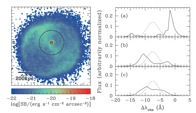
We randomly chose a halo in the simulation box, which has a mass of $\sim 10^{11}h^{-1}M_{\odot}$. The size of the virialized halo is about 26kpc, slightly larger than the inner circle in the left panel of Figure 1. As mentioned in § 3, Ly$\alpha$ photons are assumed to initially start from a point source, located at the halo center. The left panel of Figure 1 shows the Ly$\alpha$ surface brightness distribution after Ly$\alpha$ scattering from this source. Because of the radiative transfer, the initial point source becomes an extended source and a roughly spherical halo of scattered Ly$\alpha$ photons emerges. This scattered Ly$\alpha$ halo is similar to the one around a point source before reionization described in Loeb & Rybicki (1999). While Loeb & Rybicki (1999) assume a uniform, zero temperature IGM undergoing Hubble expansion, we use a realistic distribution of gas density, temperature, and velocity around a star-forming halo. This causes deviations from spherical symmetry in the surface brightness profile. The scattered Ly$\alpha$ surface brightness drops as the radius increases. The blue-green extended Ly$\alpha$ emission seen in Figure 1 is out in the IGM, corresponding to the scattered photons as they travel to the region where the Hubble expansion compensates for their blueshift acquired by the scatterings in the infall region of the halo. The sharp edge around a radius of $\sim$0.5Mpc reflects the frequency of the “bluest” photons coming out of the central (infall) region before encountering the IGM. The bluer the photons are, the farther they can travel in the IGM before redshifted to the line center and significantly scattered. In practice, we can only observe the very inner part of the extended Ly$\alpha$ radiation, where the surface brightness is high. The extended Ly$\alpha$ halo would merge with those from neighboring sources, forming a Ly$\alpha$ background. We will describe how we identify sources in the simulation in § 5.1.

In the right panels of Figure 1, we show Ly$\alpha$ spectra at different radii of the source. The dotted curve in each panel is the intrinsic Ly$\alpha$ line profile, assumed to be Gaussian with the width determined by the virial temperature of the dark matter halo hosting the source. It would be the observed spectrum if Ly$\alpha$ photons streamed out of the source without any scatterings. Note that the wavelength shown in the plot is the difference from $(1+z)\lambda_{0}$, where $z=5.7$ and $\lambda_{0}$=1216Åis the rest-frame wavelength of Ly$\alpha$ . The offset of the peak of the initial line profile from zero is caused by a combination of the Hubble velocity with respect to the center of the simulation box and the peculiar velocity of the source. On average, Ly$\alpha$ photons are first scattered by neutral hydrogen atoms in the infall region around the LAE host halo (see § 7 and Fig. 20). The inner infall region has an inverted Hubble-like contraction velocity distribution and Ly$\alpha$ photons escaping at the radius of maximum infall velocity have their frequency most likely shifted to the blue side of the line center (Zheng & Miralda-Escudé, 2002). Then Ly$\alpha$ photons experience scatterings in the region with decreasing infall velocity (outer infall region) and finally hit the Hubble flow. The subsequent scatterings on average shift the frequency of Ly$\alpha$ photons redward.

Most of the observed Ly$\alpha$ photons from regions with high surface brightness near the center of the source shift to the red side (Fig. 1$a$) with respect to the intrinsic distribution. These photons are most likely to have had forward scatterings along the line of sight. The outward increasing gas velocity (from the outer infall region and the Hubble flow) makes it easier for photons that have redward frequency shifts to escape. At larger lateral radii, (Fig. 1$b$ and Fig. 1$c$), we have more contributions from photons that travel perpendicular to the line of sight but are scattered to the line-of-sight direction. The frequency after scattering would be near the incoming frequency seen in the rest-frame of the atom at the scattering radius. Since most of the scatterings would happen around the radius where the Hubble expansion velocity redshifts the Ly$\alpha$ photons to the line-center frequency and the line-of-sight neutral column density become smaller at larger radii, the observed photons at large projected radii would appear bluer than those observed near the center, as seen in the spectra at large radii.

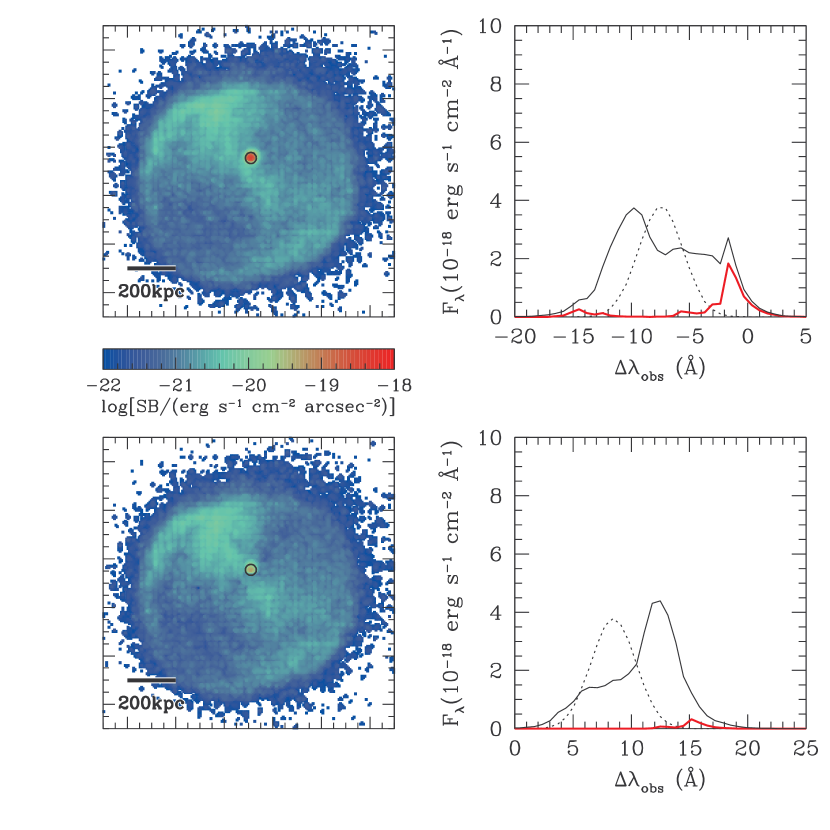
Only the very central part of the extended Ly$\alpha$ radiation can be practically observed as the LAE source. The transmitted Ly$\alpha$ flux depends on the gas distribution and kinematics in the halo vicinity, and the viewing angle. We perform a few tests to see the influence of the gas properties in the observed flux of the central part. Figure 2 compares Ly$\alpha$ images and spectra of the above source observed in two opposite directions. Mirroring reflection has been applied to one image so that the two images have the same orientation. While the two images have similar spatial extent, there is a large difference (about a factor of 7) in the flux inside the central aperture. The difference can be clearly seen from the spectra. The red curve in each of the right panels is the spectrum extracted from the circular aperture near the source center.

Evidently, the differences in the intervening gas distribution, namely the neutral hydrogen density and peculiar velocity distributions, have a dramatic effect on the observed Ly$\alpha$ flux. To test this we perform a scattering calculation with the peculiar velocities of the source and neutral gas set to zero, while keeping the Hubble expansion. Figure 3 compares the resultant images and spectra observed in the two opposite directions. Any remaining differences between the results of different viewing directions should be caused only by the anisotropic density or temperature distribution around the source. We see that, with the peculiar velocity field turned off, the difference in the fluxes from the central aperture between the two lines of sight becomes much smaller, a factor of $\sim 1.5$ (versus $\sim 7$ in the case with peculiar velocity). The spectra from the central aperture also look more similar to each other.

With the peculiar velocity turned off, the surface brightness profile of scattered Ly$\alpha$ photons appears to be more concentrated than that in Figure 2. This is mainly a consequence of the disappearance of the infall region around the source by artificially setting the peculiar velocity to zero. If the peculiar velocity is not switched off, Ly$\alpha$ photons climbing out of the infall region (before reaching the IGM dominated by the Hubble expansion) would on average have shifted blueward (Zheng & Miralda-Escudé, 2002) with respect to the line center. Compared to the case without the blueward shift (e.g., the initial Gaussian profile when the peculiar velocity is turned off), these bluer photons would travel a larger distance in the IGM before redshifting back to the line center and experiencing strong scatterings. Therefore, we see a more extended Ly$\alpha$ emission in the case with the peculiar velocity.

The above tests show that peculiar velocity plays an important role in the scattered Ly$\alpha$ brightness profile and the transmitted flux near the source center. In § 7, in additional to the peculiar velocity, we identify other factors in affecting the Ly$\alpha$ transmission and statistically study their role in the observability of LAEs.

Figure 4.— Scattered Ly$\alpha$ emission from LAEs. The Ly$\alpha$ surface brightness distribution is shown for sources in one third of the simulation box, with 100$h^{-1}{\rm Mpc}$ on a side and a thickness of 33.33$h^{-1}{\rm Mpc}$. The area matches that of the SXDS and the depth corresponds to the width of the narrow-band filter for $z\sim 5.7$ LAEs (Ouchi et al., 2008). The morphology and spectra of three sources in the zoom-in region are shown.

Figure 5.— Images and spectra of a few $z\sim 5.7$ LAE sources in our model. In each of the panels of spectra, the dotted curve is the intrinsic line profile, which would be observed if Ly$\alpha$ photons escaped without scattering. The black solid curve is the spectrum in our model with the full Ly$\alpha$ radiative transfer. For comparison, the solid red curve is the spectrum with a simple treatment of radiative transfer, which modifies the intrinsic profile by multiplying $\exp(-\tau_{\nu})$ with $\tau_{\nu}$ the line-of-sight optical depth. For an easy comparison across panels, in each panel, all three spectra have the same constant horizontal shift so that the line center of the intrinsic profile is at zero. In each spectra panel, the label starting with “M” denotes $\log(M_{h})$, where the host halo mass $M_{h}$ is in units of $h^{-1}M_{\odot}$. See text for details.

The results from the individual LAE source show that, as a consequence of radiative transfer, Ly$\alpha$ photons experience both spatial diffusion and frequency diffusion. An intrinsic point source of Ly$\alpha$ emission appears extended and the Ly$\alpha$ spectra differ substantially from the intrinsic Gaussian profile. The spectra from the central aperture, which is the part that is most observable, do not have a simple and clear relation to the initial line profile, owing to the frequency shift caused by scatterings. In some previous work (e.g., McQuinn et al. 2007; Iliev et al. 2008), the observed Ly$\alpha$ spectrum is modeled as the intrinsic Gaussian profile modified by $\exp(-\tau_{\nu})$ with $\tau_{\nu}$ being the optical depth at frequency $\nu$ along the line of sight. Such a simple model does not account for the frequency and spatial diffusion of Ly$\alpha$ photons caused by radiative transfer. The resultant line profile in this simple model looks like a truncated Gaussian profile, with only the red tail transmitted. Our detailed Ly$\alpha$ radiative transfer, on the other hand, shows that the observed Ly$\alpha$ line profile near the source center is more complicated and the redward frequency shift is more than that in the simple treatment. The simple radiative transfer model may yield trends in some results that are qualitatively in accord with detailed transfer calculations. For example, Iliev et al. (2008) also find that peculiar velocity is important in determining the observability of LAEs. However, as we show in § 5, the lack of frequency and spatial diffusion in the simple model means that it cannot capture the full picture of Ly$\alpha$ emission from LAEs for detailed prediction and understanding of observed Ly$\alpha$ features.

5. Statistical Properties of Ly$\alpha$ Spectra and Luminosity of LAEs

We perform Ly$\alpha$ scattering calculation for all the sources residing in halos above $5\times 10^{9}h^{-1}M_{\odot}$ in the whole $(100h^{-1}{\rm Mpc})^{3}$ box. In this section, we describe how we identify LAEs from the post-scattering outputs and study their statistical properties.

5.1. Source Identification

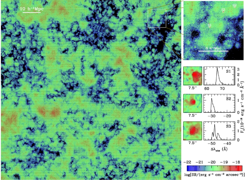
Figure 4 shows the Ly$\alpha$ image for sources in one-third of the simulation box. It has an area of 100$h^{-1}{\rm Mpc}\times$100$h^{-1}{\rm Mpc}$ and a thickness of 33.33$h^{-1}{\rm Mpc}$. The slice matches the sky coverage (1 deg²) of the SXDS and the depth corresponds to the width of the narrow-band filter ($\Delta\lambda$=120Å; Ouchi et al. 2008) for $z=5.7$ LAEs. Therefore, the image can be regarded as an idealized, continuum-subtracted narrow band image of the $z=5.7$ LAEs for SXDS-like sky coverage and depth. From the whole simulation box, we have three realizations of such a survey. The periodic boundary condition of the simulation is imposed in our modeling, which can be clearly seen in Figure 4.

Because of Ly$\alpha$ radiative transfer, LAEs are no longer point sources in our model. We need to find a way to define the sources in order to study their statistical properties. Our identification of sources is motivated by the procedure used in detecting LAEs in real observations. For $z=5.7$ LAEs in the SXDS, a threshold surface brightness of $2.64\times 10^{-18}{\rm erg\,s^{-1}\,cm^{-2}\,arcsec^{-2}}$ in the narrow-band image (including continuum) is adopted for detecting them (M. Ouchi, private communication). LAEs are identified by grouping pixels above this threshold. The observed rest-frame Ly$\alpha$ equivalent width distribution of $z\sim 5.7$ LAEs peaks around 60Åand is skewed to large values (Fig.23 in Ouchi et al. 2008). Since the rest-frame width of the narrow-band filter is 120Å/$(1+z)$, the continuum contribution to the surface brightness are likely to be less than 30%. Our model does not include the continuum component. In principle, we could model the continuum based on the star formation history in the simulation, but the correction is small and it is not the main uncertainty of our model (as shown later in this paper). Therefore, we simply make a correction of 1/3 to remove the continuum contribution to the threshold surface brightness and adopt $1.80\times 10^{-18}{\rm erg\,s^{-1}\,cm^{-2}\,arcsec^{-2}}$ as the continuum-subtracted surface brightness for detecting SXDS LAEs.

Figure 6.— The apparent shift in the LAE Ly$\alpha$ line peak with respect to the intrinsic one. Because of radiative transfer, the wavelength $\lambda_{\rm peak}$ at the peak flux of the observed Ly$\alpha$ line is not $\lambda_{c}$ that corresponds to the center of the intrinsic (Gaussian) line profile. The apparent shift is defined as the wavelength difference. The top axis of the left panel marks the shift in comoving unit, which is of the order of $h^{-1}{\rm Mpc}$. Left: The distribution of the apparent shift of the peak wavelength as a function of LAE host halo mass (in units of $h^{-1}M_{\odot}$). The apparent wavelength shift can translate to an apparent shift in the redshift-space source position $\Delta Z$ along the line of sight, which is labeled in the top axis. Right: Similar to the left panel, but the peak wavelength shift is in units of the intrinsic line width $\sigma_{\lambda}$, which is set by the virial temperature of the host halo in our model.

Figure 7.— Similar to the left panel of Fig. 6, but for the apparent shift in the LAE Ly$\alpha$ line peak as a function of the observed (apparent) Ly$\alpha$ luminosity (in units of ${\rm erg\,s^{-1}}$).

As shown in § 6, there is significant uncertainty in modeling Ly$\alpha$ luminosity. To be conservative, we set a lower threshold surface brightness, $1.8\times 10^{-19}{\rm erg\,s^{-1}\,cm^{-2}\,arcsec^{-2}}$, for identifying LAEs in our model. To have a full picture of the observability of LAEs (e.g., comparison between intrinsic and observed Ly$\alpha$ emission), we also include the halo position information in the source identification. For a source with the projected position known from the halo catalog, we first find the corresponding pixel in the Ly$\alpha$ image. Starting from this root pixel, we then link the surrounding pixels with surface brightness above the threshold through a Friends-of-Friends (FoF) algorithm with the linking length equal to the size of the pixel. The directions to link the pixels are only horizontal and vertical in the image. An LAE source is then defined by all the linked pixels, and the spectra at each pixel’s position are added together to form the spectra of the source. In the case that the root pixel and its surrounding pixels all have surface brightnesses lower than the threshold, the flux and spectra from this root pixel are adopted for the source. As with other applications of the FoF algorithm, there are chances that two individual sources are bridged together. In this case, we also assign the flux and spectra of the root pixel to the intrinsically fainter source. Such cases are rare and the correction does not affect any of our statistical study.

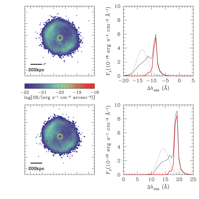
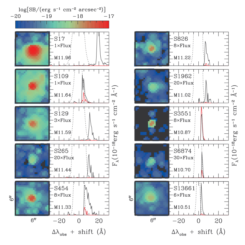
Figure 5 shows Ly$\alpha$ images and spectra of a few $z\sim 5.7$ LAEs from our model. The host halo masses of these sources are above $3\times 10^{10}h^{-1}M_{\odot}$. The corresponding intrinsic Ly$\alpha$ luminosities are above $2\times 10^{42}{\rm erg\,s^{-1}}$ (equations [1] and [2]), roughly in the luminosity range probed by current LAE surveys like SXDS. From top to bottom panels and left to right panels, they are arranged in order of decreasing intrinsic Ly$\alpha$ luminosity (halo mass). Most of the sources appear to be roughly round with faint substructures around them, which are a combination of reflected Ly$\alpha$ emission by clumps/filaments of neutral gas or Ly$\alpha$ emission from fainter sources. The sizes and morphologies of the LAEs in our model are remarkably similar to those in the narrow-band images of $z\sim 5.7$ LAEs in SXDS (e.g., Fig.5 of Ouchi et al. 2008; narrow-band images in Fig.3 of Taniguchi et al. 2009).

Solid curves in the spectrum panels in Figure 5 are the corresponding spectra for the shown LAEs. In each spectrum, the Ly$\alpha$ line is clearly asymmetric, skewed towards the red. The line profiles resemble the observed ones for the SXDS $z\sim 5.7$ LAEs (Fig.5 of Ouchi et al. 2008). However, the observed Ly$\alpha$ lines appear to be much broader with less sharp blue edges. The difference can be simply attributed to the spectral resolution: in the observer’s frame, the observation typically has a resolution 8–15Å(Ouchi et al., 2008), while the resolution for our modeled spectra is 0.67Å.

The Ly$\alpha$ lines with the full radiative transfer show a clear distinction from the lines with a simple treatment of the radiative transfer, namely the $\exp(-\tau_{\nu})$ model. For each source, the red curve is the Ly$\alpha$ spectrum from the $\exp(-\tau_{\nu})$ model, which is essentially the intrinsic Gaussian profile truncated below a certain wavelength. Although it displays a similar asymmetry, the flux is usually significantly lower than that with the full radiative transfer. Importantly, the Ly$\alpha$ line from the full radiative transfer model has a larger redward shift than that in the simple model, an effect that can only be properly modeled with detailed radiative transfer calculations. This is primarily because detailed radiative transfer leads to frequency diffusion, causing some of the original photons closer to the line center to diffuse out to the wings. The shift in frequency not only results in smaller scattering optical depth but also is accompanied by spatial diffusion, both leading to larger transmitted flux near the center.

5.2. Shift in the Peak of Ly$\alpha$ Spectra

Figure 8.— Relation between the observed (apparent) and the intrinsic Ly$\alpha$ luminosities of LAEs. Panel (a): The joint distribution of apparent and intrinsic Ly$\alpha$ luminosities. Adjacent contours differ by a factor of 2 in contour levels. A vertical cut in this plot gives the probability distribution function (PDF) of apparent luminosity at a given intrinsic luminosity [Panel (b)], and a horizontal cut gives the distribution of intrinsic luminosity at a given apparent luminosity [Panel (c)]. Only halos above $5\times 10^{9}h^{-1}M_{\odot}$ are considered in our model, which corresponds to intrinsic luminosity above $\sim 10^{41.5}{\rm erg\,s^{-1}}$. As a results, the apparent luminosity is complete above $\sim 10^{41.2}{\rm erg\,s^{-1}}$.

Figure 9.— Correlation between apparent to intrinsic luminosity ratio and wavelength shift at peak Ly$\alpha$ flux. The peak wavelength shift is in units of the intrinsic line width $\sigma_{\lambda}$, which is set by the virial temperature of the host halo in our model. Contours show the correlation and they enclose the 68% and 95% distribution, respectively. The solid curve is the median wavelength shift as a function of luminosity ratio. The two dotted curves delineate the upper and the lower quartiles.

Figure 10.— Comparison of the relations between the observed (apparent) and the intrinsic Ly$\alpha$ luminosities from different models. The dotted contours are from our model with full calculation of Ly$\alpha$ radiative transfer (the same contours as in Fig. 8$a$). The solid contours in panel ($a$) are from the simple $\exp(-\tau_{\nu})$ model with the initial Ly$\alpha$ line width given by halo virial temperature, as adopted in our model with full radiative transfer calculation. The solid contours in panel ($b$) are also from the $\exp(-\tau_{\nu})$ model, but the initial Ly$\alpha$ line width is determined by the circular velocity at halo virial radius, which is about 2.3 times larger than the one adopted in panel ($a$). Note that the $\exp(-\tau_{\nu})$ model and the full calculation in panel ($b$) assume different initial Ly$\alpha$ line widths, so it is not an apple-to-apple comparison. It shows that modifying the initial line width of the $\exp(-\tau_{\nu})$ model does not lead to a result mimicking that from the full calculation.

Figure 11.— Comparison between the apparent-to-intrinsic Ly$\alpha$ luminosity ratios from our full radiative transfer calculation (full RT) and the $\exp(-\tau_{\nu})$ model. The thin solid curve shows the median ratio from the $\exp(-\tau_{\nu})$ model as a function of the ratio from the full RT for halos below $10^{10.5}h^{-1}M_{\odot}$. The two thin dotted curves indicate the lower and upper quartiles. The set of thick curves are for halos above $10^{10.5}h^{-1}M_{\odot}$. The diagonal dashed line is the line of equality.

Figure 12.— Comparison of the correlation between apparent to intrinsic luminosity ratio and peak wavelength shift from different models. The dotted contours are from our model with full calculation of Ly$\alpha$ radiative transfer (the same contours as in Fig. 12). The solid contours on the left are from the simple $\exp(-\tau_{\nu})$ model with the initial Ly$\alpha$ line width given by halo virial temperature, as adopted in our model with full radiative transfer calculation. The solid contours on the right are also from the $\exp(-\tau_{\nu})$ model, but the initial Ly$\alpha$ line width is determined by the circular velocity at halo virial radius, which is about 2.3 times larger than the one from halo virial temperature. For all the three sets of contours, the peak wavelength shift is in units of the line width $\sigma_{\lambda}$ set by halo virial temperature. The two contours in each case show the 68% and 95% distribution, respectively.

Together with the assumed intrinsic properties, LAEs identified in the post-scattering IFU-like data cube from our model enable a statistical study of the relations between the observed and intrinsic quantities, which include spectral features and luminosity.

As shown in Figure 5, owing to radiative transfer effect, the peak in the observed Ly$\alpha$ spectra is at a wavelength longer than that in the intrinsic spectra. In the left panel of Figure 6, we plot the distribution of the shift as a function of host halo mass. The broad distribution of the shift reflects the distribution of circumgalactic and intergalactic environments (density and velocity structures), which affect the radiative transfer of Ly$\alpha$ photons (see § 7). This apparent wavelength shift in the peak depends on host halo mass, or intrinsic luminosity of the source given that star formation rate is tightly correlated with halo mass in the reionization simulation. In general, the distribution is skewed to large shifts. For sources in lower mass halos, the distribution is narrower and the average shift is smaller. For sources in halos of $\sim 10^{10}h^{-1}M_{\odot}$, the median shift corresponds to a velocity of $\sim 70{\rm km\,s^{-1}}$, while for $\sim 10^{11}h^{-1}M_{\odot}$ halos, the value is $\sim 200{\rm km\,s^{-1}}$. If the observed Ly$\alpha$ emission was from photons backscattered from the far side of galactic wind (e.g., Franx et al., 1997; Adelberger et al., 2003), the above shift would lead to an overestimate of the wind velocity as long as it is estimated by the apparent velocity difference between the Ly$\alpha$ emission and optical emission/absorption lines. The apparent wavelength shift also translates to a shift in the apparent position/redshift of the source along the line of sight (top axis of the left panel of Fig. 6). This position shift and its scatter would result in slight distortion and smoothing in the clustering of LAEs in redshift space (see Paper II for more details).

In the right panel of Figure 6, the apparent shift of the Ly$\alpha$ line peak is put in units of the intrinsic Ly$\alpha$ line width $\sigma_{\lambda}$, which is assumed to be determined by the halo virial temperature. Although the trends seen in the left panel are still evident, the variation of the distribution as a function of halo mass becomes weaker. Roughly speaking, the median shift is about $3\sigma_{\lambda}$ and the scatter is about 0.6–0.9$\sigma_{\lambda}$. In terms of velocity, the median shift is approximately $100[M_{h}/(10^{10}h^{-1}M_{\odot})]^{1/3}\,{\rm km\,s^{-1}}$.

The distribution of Ly$\alpha$ peak shift we discuss so far is as a function of intrinsic Ly$\alpha$ luminosity (i.e., halo mass). From the point of view of observation, it is of great interest to show the distribution as a function of the observed Ly$\alpha$ luminosity. Figure 7 plots the distribution of Ly$\alpha$ peak shift as a function of observed (apparent) Ly$\alpha$ luminosity. As shown later in § 5.3, at fixed intrinsic Ly$\alpha$ luminosity, the observed (apparent) Ly$\alpha$ luminosity has a broad distribution, and vice versa. The peak shift distribution at fixed observed luminosity is therefore contributed by sources residing in halos of a broad range of mass. We note that the model luminosity in the plot should be increased by about 0.7 dex to match the $z\sim 5.7$ observation (see § 6).

5.3. Apparent and Intrinsic Ly$\alpha$ Luminosities

The observed Ly$\alpha$ flux $F_{{\rm Ly}\alpha}$ from an LAE source in the narrow-band image comes from the central part, where the surface brightness is high. That is, only a fraction of the extended radiation composed of scattered Ly$\alpha$ photons can be observed. The observationally inferred Ly$\alpha$ luminosity $L_{\rm apparent}=4\pi D_{L}^{2}F_{{\rm Ly}\alpha}$ is therefore expected to be lower than the intrinsic Ly$\alpha$ luminosity $L_{\rm intrinsic}$, where $D_{L}$ is the luminosity distance and isotropic emission is assumed in computing the apparent luminosity from the observed flux.

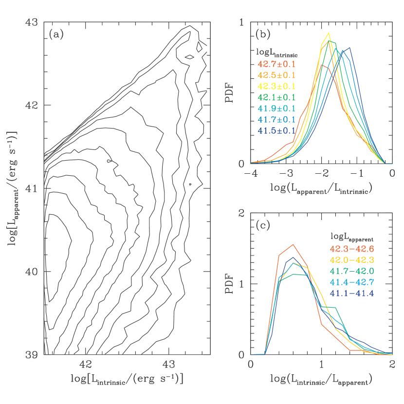
We compare the intrinsic and apparent Ly$\alpha$ luminosities in our model. Figure 8$a$ gives the joint distribution of $L_{\rm intrinsic}$ and $L_{\rm apparent}$. From the joint distribution, we can obtain the distribution of $L_{\rm apparent}$ at a fixed $L_{\rm intrinsic}$ or vice versa, through a vertical or horizontal cut. Since we only model LAEs in halos above $5\times 10^{9}h^{-1}M_{\odot}$, we are limited to sources with $L_{\rm intrinsic}$ above $\sim 10^{41.5}{\rm erg\,s^{-1}}$. When considering the observed luminosity, sources are complete for $L_{\rm apparent}\gtrsim 10^{41.2}{\rm erg\,s^{-1}}$. We note that the Ly$\alpha$ luminosity limits may change if the assumed IMF and SFR differ from those in our model.

In the luminosity range probed by our model, the apparent Ly$\alpha$ luminosity peaks at a few percent of the intrinsic one and is broadly distributed (Fig.8$b$). The scatter reflects differences in neutral gas distributions (density, velocity, and temperature) around sources of the same intrinsic luminosity (§ 7). The distribution shifts slightly towards higher values for sources of lower intrinsic luminosity. If we define the ratio of the apparent to intrinsic luminosity as flux suppression, the suppression on average appears to be smaller for intrinsically fainter sources, which seems counter-intuitive. Such a shift is a consequence that the environment of low mass halos are on average less dense than that of massive halos, and that the environment is important in shaping the observability, to be discussed in detail in § 7.

From the point of view of observation, it is interesting to ask what the observed Ly$\alpha$ luminosity implies about the intrinsic one. Figure 8$c$ shows the intrinsic luminosity distribution at a given apparent luminosity. The distributions for different values of $L_{\rm apparent}$ are similar in terms of the intrinsic to apparent luminosity ratio. In general, the intrinsic luminosity is about 3–12 times the observed luminosity. In other words, a large fraction of the escaped Ly$\alpha$ photons are invisible. For estimating Ly$\alpha$ escape fraction from observations, this is a systematic factor that needs to be taken into account.

We find that the flux suppression is correlated with the shift in the peak of Ly$\alpha$ profile (§ 5.2), as shown in Fig.9. For sources with a larger suppression in Ly$\alpha$ flux, the peak of the spectra shifts more towards red. This correlation has only a weak dependence on halo mass or intrinsic luminosity and in Figure 9 all sources in our model are included. Clearly, the correlation is a consequence of the radiative transfer: Ly$\alpha$ photons diffuse more in frequency as they experience more scatterings. The correlation is driven by the dependence of the Ly$\alpha$ radiative transfer on environments, i.e., the circumgalactic and intergalactic density and velocity structures (see § 7).

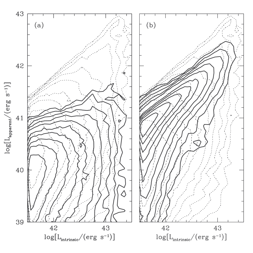
It is worth pointing out that the simple $\exp(-\tau_{\nu})$ model can only give qualitatively trends seen in our results. In Figure 10, we compare the $L_{\rm apparent}$–$L_{\rm intrinsic}$ distribution from our model of full radiative transfer with those from the $\exp(-\tau_{\nu})$ model. The $\exp(-\tau_{\nu})$ model in Figure 10$a$ assumes the same intrinsic Ly$\alpha$ line width as in our model, which is set by halo virial temperature. It is evident that at the same intrinsic Ly$\alpha$ luminosity, the $\exp(-\tau_{\nu})$ model leads to much lower apparent Ly$\alpha$ luminosities than the full calculation. In particular, the suppression from the $\exp(-\tau_{\nu})$ model becomes much stronger for sources of higher intrinsic Ly$\alpha$ luminosity (or halo mass) because of the high density and peculiar velocity. The trend is similar to what Iliev et al. (2008) find. As they point out, peculiar velocity plays an important role in shaping the luminous end of the observed Ly$\alpha$ luminosity function. The frequency and spatial diffusions in the full calculation can compensate the density and peculiar velocity effect, weakening the suppression. Compared to the $\exp(-\tau_{\nu})$ model, the suppression from the full calculation does not become much stronger for sources of higher intrinsic Ly$\alpha$ luminosity (also see Figure 11).

The $\exp(-\tau_{\nu})$ model in Figure 10$b$ adopts an intrinsic Ly$\alpha$ line width 2.3 times that used in Figure 10$a$, which corresponds to the circular velocity at halo virial radius. This value of intrinsic line width is used in some previous work (e.g., McQuinn et al., 2007; Iliev et al., 2008) with the $\exp(-\tau_{\nu})$ model. This model boosts the apparent Ly$\alpha$ luminosity, but the suppression is still stronger than the full calculation at high halo mass end. In addition, the distribution of apparent Ly$\alpha$ luminosity at fixed intrinsic Ly$\alpha$ luminosity is much narrower than that from the full calculation. We do not have results from a full radiative transfer calculation with the larger intrinsic Ly$\alpha$ line width yet, but we expect that the difference between such a full calculation and the $\exp(-\tau_{\nu})$ model is similar to that seen in Figure 10$a$. We caution that Figure 10$b$ does not show an apple-to-apple comparison, since the $\exp(-\tau_{\nu})$ model and the full calculation assume different intrinsic line widths. Nevertheless, it indicates that modifying the $\exp(-\tau_{\nu})$ by varying the intrinsic line width does not lead to a match to the full radiative transfer calculation.

To further see the difference between the full radiative transfer model and the $\exp(-\tau_{\nu})$ model with the same intrinsic Ly$\alpha$ line width setup, we compare the apparent-to-intrinsic Ly$\alpha$ luminosity ratios predicted from the two models on a one-to-one basis (Figure 11). We summarize the scatter plot by showing the median ratio (solid curve) from the $\exp(-\tau_{\nu})$ model as a function of the ratio from our model (the “true” ratio), together with the lower and upper quartiles (dotted curves). Thin and thick curves are for sources in halos below and above $10^{10.5}h^{-1}M_{\odot}$, respectively. In general, there is a trend that the ratio from the $\exp(-\tau_{\nu})$ model increases with the “true” value and this trend seems to break down in massive halos at high values of the “true” ratio. In a limited range (around $L_{\rm apparent}/L_{\rm intrinsic}\sim 10^{-2}$), the median ratio from the $\exp(-\tau_{\nu})$ appears to be a constant shift from the “true” ratio. However, even if we apply a correction to account for the shift, the $\exp(-\tau_{\nu})$ model would underpredict the luminosity ratio outside of the above narrow range, in particular towards higher values of the “true” ratio. Even within the narrow range, the ratio from the $\exp(-\tau_{\nu})$ model has a large scatter (a factor of a few) at a fixed “true” ratio.

The Ly$\alpha$ flux suppression in our $\exp(-\tau_{\nu})$ model appears to be much stronger than seen in previous work (e.g., McQuinn et al., 2007; Iliev et al., 2008). Compared to our work, previous work assumes a much wider initial Ly$\alpha$ line width and lower gas temperature (set to be $10^{4}$K). The differences in the above two factors largely explains the differences in the results. For more detailed explanations and discussions, see Appendix A, where we perform several tests with the $\exp(-\tau_{\nu})$ model by varying the initial Ly$\alpha$ line width and gas temperature.

Figure 12 compares the correlation between apparent to intrinsic luminosity ratio and peak wavelength shift from our full radiative transfer model (dotted contours) and the above two $\exp(-\tau_{\nu})$ models (solid contours). Although the sign of the correlation is the same for all three models, the $\exp(-\tau_{\nu})$ model with smaller (larger) intrinsic Ly$\alpha$ line width gives a smaller (larger) slope in the correlation than the full calculation.

The comparisons with the $\exp(-\tau_{\nu})$ model results in this section demonstrate that the $\exp(-\tau_{\nu})$ model can provide a qualitative understanding of the results, but there is no simple way to modify the results from the $\exp(-\tau_{\nu})$ model to match those of the full calculation. Full radiative transfer calculation is necessary to obtain quantitatively correct results in Ly$\alpha$ emission properties of LAEs.

5.4. Ly$\alpha$ Luminosity Function of LAEs

An important product of surveys of LAEs is the Ly$\alpha$ LF, one of the most widely studied statistical properties of LAEs. The LF can be used to infer the relation between LAEs and their host dark matter halos. The evolution of LFs around the reionization epoch can probe the reionization of the universe (e.g., Malhotra & Rhoads, 2004; Haiman & Cen, 2005). As we have shown in § 5.3, the observed Ly$\alpha$ luminosity of LAEs differ from the intrinsic one. Here we study the Ly$\alpha$ LF of LAEs from our model.

The star formation prescription adopted in the reionization simulation leads to a tight correlation between star formation rate and halo mass. Therefore the intrinsic Ly$\alpha$ luminosity is tied to the halo mass and the intrinsic Ly$\alpha$ LF largely reflects the halo mass function. In Figure 13, the filled squares show the intrinsic Ly$\alpha$ LF, $\Phi_{i}(L_{\rm intrinsic})$. The apparent Ly$\alpha$ LF, $\Phi_{a}(L_{\rm apparent})$, is related to the intrinsic one through

$$\Phi_{a}(L_{\rm apparent})=\int_{0}^{\infty}p(L_{\rm apparent}|L_{\rm intrinsic})\Phi_{i}(L_{\rm intrinsic})dL_{\rm intrinsic},$$ (3)

where $p(L_{\rm apparent}|L_{\rm intrinsic})$ is the probability density of the apparent luminosity at a given $L_{\rm intrinsic}$ (Fig. 8$b$). The apparent Ly$\alpha$ LF can be directly read off from Figure 8$a$ and is shown as open squares in Figure 13. In terms of luminosity, the apparent Ly$\alpha$ LF shifts towards the faint end by a factor of 5–20 with respect to the intrinsic one and the shift is larger at the faint end. Formally, the intrinsic LF can be inferred from the observed one by

$$\Phi_{i}(L_{\rm intrinsic})=\int_{0}^{\infty}p(L_{\rm intrinsic}|L_{\rm apparent})\Phi_{a}(L_{\rm apparent})dL_{\rm apparent},$$ (4)

where $p(L_{\rm intrinsic}|L_{\rm apparent})$ is the probability density of the intrinsic luminosity at a given $L_{\rm apparent}$ (Fig. 8$c$). However, even if $p(L_{\rm intrinsic}|L_{\rm apparent})$ is known or assumed a priori, it is not enough to infer the intrinsic LF from the observed one. The reason is that at a given intrinsic luminosity, the distribution of apparent luminosity can have a tail to low value (Fig. 8). So one needs to have observations of the apparently faint LAEs to recover the full information of the intrinsic luminosity distribution, or one has to rely on the extrapolation of the observed LF to the faint end.

Figure 13.— Ly$\alpha$ luminosity function of $z\sim 5.7$ LAEs. The intrinsic luminosity function in our model is represented by filled squares. The apparent luminosity function from a full radiative transfer calculation is plotted as open squares. For comparison, the crosses show the apparent luminosity function with a simple $\exp(-\tau_{\nu})$ radiative transfer treatment. Poisson errors are plotted.

For comparison, the crosses in Figure 13 show the Ly$\alpha$ LF from the $\exp(-\tau_{\nu})$ model, which adopts the same intrinsic Ly$\alpha$ line width as the full radiative transfer calculation. As already demonstrated in § 5.3, the Ly$\alpha$ flux is more strongly suppressed in the $\exp(-\tau_{\nu})$ model. The resultant apparent Ly$\alpha$ LF looks like the intrinsic one shifting toward the faint end by more than two orders of magnitude in luminosity. With the same intrinsic Ly$\alpha$ LF, the apparent Ly$\alpha$ LF from the full radiative transfer model is significantly higher than that from the $\exp(-\tau_{\nu})$ model, a consequence of the frequency and spatial diffusion of Ly$\alpha$ photons from scatterings.

6. Implications for Observed Properties of LAEs

Our model of LAEs predicts the relation between observed Ly$\alpha$ emission and the intrinsic one. With simple assumptions about the intrinsic properties of LAEs, we are able to predict an array of observational properties of LAEs. In this section, we compare our model predictions to observations for $z\sim 5.7$ LAEs and attempt to understand various observed properties of LAEs. We focus here on the Ly$\alpha$ LF, the UV LF, and the Ly$\alpha$ equivalent width (EW) distribution of LAEs.

6.1. Ly$\alpha$ Luminosity Function

Figure 14.— Observed Ly$\alpha$ LF of $z\sim 5.7$ LAEs. Solid circles connected by solid lines are the observed LF for $z\sim 5.7$ LAEs in the 1 deg² SXDS (Ouchi et al., 2008). Open circles connected by dotted lines are the observed one from the 0.2 deg² Subaru Deep Field (a different sky area from SXDS; Shimasaku et al. 2006). Open squares are the apparent LF from our model with a full radiative transfer calculation, and diamonds are the same but with the Ly$\alpha$ luminosity boosted by a factor of 5 (see text for details).

In our model, the apparent Ly$\alpha$ luminosity corresponds to the observed one. The open squares in Figure 14 (the same as in Fig. 13) show the predicted Ly$\alpha$ LF of LAEs from the model. Filled circles are the measurement based on 401 LAEs from the 1 deg² SXDS (Ouchi et al., 2008), while open circles show that based on 89 LAEs in a 0.2 deg² Subaru Deep Field (Shimasaku et al., 2006) that covers a different sky area from SXDS.

Compared with the observed Ly$\alpha$ LF, the apparent LF from our model appears to be one order of magnitude lower in normalization. This seems to put into question our model. However, the normalization is not necessarily a good indicator of the importance of the difference. A more sensible way is to characterize the difference by the shift in luminosity scale — with respect to the observed Ly$\alpha$ LF, the apparent LF from our model is shifted by a factor of 3–6 to the left (toward the low luminosity end). If we simply increase the apparent Ly$\alpha$ luminosity by a factor of 5, the apparent LF (shown as diamonds in Fig. 14) shows a better match to the observed one. The factor of 3–6 discrepancy between the model and the data implies that we are missing some physics in our modeling. For comparison, the apparent Ly$\alpha$ LF based on the simple $\exp(-\tau_{\nu})$ model (crosses in Fig. 13) corresponds to about two orders of magnitude shift in luminosity with respect to the observed one. Again, the frequency and spatial diffusion from the realistic radiative transfer in our model enhances the probability of being detected for Ly$\alpha$ photons.

Before discussing possible solutions to the factor of 3–6 shift in luminosity, we justify that changing the normalization of Ly$\alpha$ LF cannot be the solution for the discrepancy. The normalization can only be changed by changing the amplitude of the halo mass function. However, we do not expect a large uncertainty in the latter with the current constraints on cosmology. The reionization simulation that our model is based on adopted cosmological parameters in accordance with WMAP five-year results. To estimate the cosmology-caused change in the halo mass function, we make use of the analytic formula given by Sheth & Tormen (1999). Not surprisingly, the uncertainty in $\sigma_{8}$ dominates the amplitude change in the halo mass function. Within the 1-$\sigma$ uncertainties of the WMAP five-year cosmological parameters (Dunkley et al., 2009), the cosmological parameters used in the simulation already put the halo mass function amplitude in the high end. Different combinations of cosmological parameters within their 1-$\sigma$ uncertainty ranges can only boost the amplitude by $\sim 30\%$. Therefore, we conclude that cosmology-caused amplitude change in halo mass function does not help much in making our model Ly$\alpha$ LF match the observed one.

Ly$\alpha$ luminosity depends on the amount of massive stars that emit ionizing photons. The conversion from star formation rate to intrinsic Ly$\alpha$ luminosity adopted in our model assumes Salpeter (1955) IMF. For a fixed total stellar mass with star mass distributed in the range of 0.1–100$M_{\odot}$, simply changing to a Chabrier (2003) IMF, which has shallower slopes than the Salpeter IMF below a characteristic mass of 1$M_{\odot}$, can increase the ionizing photons by a factor of $\sim$1.6. This assumes no evolution in the stellar IMF with cosmic time. Recent studies (e.g., Davé 2008; van Dokkum 2008) show evidence of an evolving IMF and observations of $z\sim$7 dropout galaxies also implies an IMF changes towards high redshift (e.g., Ouchi et al., 2009). The form of evolution can be thought as an increasing characteristic mass in the Chabrier IMF with increasing redshift. By adopting either form of the IMF at high redshift proposed by Davé (2008) and van Dokkum (2008), we find an increase in the ionizing photons by a factor of $\sim$5.5 with respect to the Salpeter IMF. Therefore, for the instantaneous star formation rate, the Ly$\alpha$ luminosity could have the amount of enhancement we need for the model prediction to match the observation. Obviously, the situation is not as simple as this and there are additional factors, such as the dependence on star formation history and metallicity. Overall, a possible factor of 3–6 in underestimating the intrinsic Ly$\alpha$ luminosities in our present model may be physically accounted for and that would put our model in accord with observations.

Figure 15.— Effect of the initial Ly$\alpha$ line width. Plotted here is the ratio of the apparent (observed) to intrinsic Ly$\alpha$ luminosity of $z\sim 5.7$ LAEs as a function of the initial Ly$\alpha$ line width $\sigma_{\rm init}$. The bottom axis marks the line width in terms of the width $\sigma_{\rm vir}$ set by halo virial temperature, while the top axis in units of the circular velocity $v_{c}$ at halo virial radius. The solid and dotted curves are the median and quartiles of the luminosity ratio distribution. This test is done with a small simulation (box size of 25$h^{-1}{\rm Mpc}$ on a side). The distribution is calculated from all sources with halo mass above $5\times 10^{9}h^{-1}M_{\odot}$. See text.

Figure 16.— UV LFs of LAEs. Left panels are for $z\sim 5.7$ LAEs. The thick solid curve is the UV LF for all galaxies in our model. The filled squares connected by the thin solid curve are the UV LF of model LAEs with the apparent Ly$\alpha$ luminosity above a threshold. The threshold is chosen so that the number density matches that of SXDS $z=5.7$ LAEs (see text). The observed UV LFs of LAEs are plotted as open symbols, obtained by Ouchi et al. (2008) (circles), Shimasaku et al. (2006) (triangles), and Hu et al. (2006) (stars), respectively. The LF of $i$–dropout galaxies at $z\sim 6$ is shown as crosses (Bouwens et al., 2006) and asterisk (Shimasaku et al., 2006). In the bottom left panel, an effective UV extinction of $A_{\rm UV,eff}=0.3$ is applied to the two curves from the model (see text). The two right panels are the observed UV LF for LAEs at $z\sim 3$ and $z\sim 4$ in SXDS, taken from Ouchi et al. (2008).

In addition, a possible increase in the intrinsic Ly$\alpha$ width may also increase the apparent luminosity. In our model, the intrinsic Ly$\alpha$ line profile is assumed to be Gaussian with width determined by the halo virial temperature. The virial temperature is defined as $T_{\rm vir}=GM_{h}\mu m_{H}/(3kR_{\rm vir})$ (Trac & Cen, 2007), resulting in a line width of $(\mu/3)^{1/2}v_{c}\simeq 0.44v_{c}$. Here $\mu\sim 0.59$ is the mean molecular weight and $v_{c}\simeq 155[M_{h}/(10^{11}h^{-1}M_{\odot})]^{1/3}{\rm km\,s^{-1}}$ the circular velocity at the virial radius. Such an assumption on the line width is conservative. Many processes can alter the intrinsic line profile. Disk rotation can change the line profile and broaden it. Galaxy merging and galactic wind from star formation can also substantially broaden the line. Many authors have adopted line width $\sim v_{c}$ or larger in computing Ly$\alpha$ transmission with the $\exp(-\tau_{\nu})$ model (e.g., Santos 2004; Dijkstra et al. 2007; McQuinn et al. 2007; Iliev et al. 2008). We have tested the effect of the initial line width by performing Ly$\alpha$ radiative transfer for LAEs in a small simulation of box size of 25$h^{-1}{\rm Mpc}$ as well as for a subset of LAEs in the 100$h^{-1}{\rm Mpc}$ box simulation. Figure 15 shows the apparent to intrinsic Ly$\alpha$ luminosity ratio as a function of the initial Ly$\alpha$ line width from the simulation with the 25$h^{-1}{\rm Mpc}$ box, inferred from all sources with halo mass above $5\times 10^{9}h^{-1}M_{\odot}$. Changing the line width we adopt to $v_{c}$ can lead to a factor of $\sim$5 increase in the median luminosity ratio. Therefore, the effect of initial Ly$\alpha$ line width can potentially shift the apparent Ly$\alpha$ LF by a factor of a few towards the bright end.

Moreover, the star formation prescription adopted in the simulation has a number of assumptions and uncertainties because of the limitation in our understanding of the baryon-related processes. A higher SFR than that in the simulation would lead to an increase in the intrinsic Ly$\alpha$ luminosity, and hence an increase in the apparent Ly$\alpha$ luminosity.

We see that a combination of changes in stellar IMF, intrinsic line width, and SFR can solve the problem of a factor of a few mismatch between the apparent Ly$\alpha$ LF of our model and the observed one. Changing the IMF and SFR would also change the reionization process and the neutral fraction of IGM, although they are degenerate with uncertain escape fraction of ionizing photons. The prediction of Ly$\alpha$ luminosity is coupled with the evolution of the gas ionization state. A self-consistent calculation is possible, but it is out of the scope of this paper. An accurate estimation of the initial Ly$\alpha$ profile and width would require detailed calculation of the Ly$\alpha$ transfer through realistic ISM of high redshift galaxies, which is little constrained and difficult to compute from first principles presently. We conclude that, owing to model uncertainties, the discrepancy between model LF and observed LF is not as serious a problem as it appears to be and may be indications of some interesting physics that is not considered in our current calculation or the need to have more accurate prescriptions of some processes.

6.2. UV Luminosity Function

As mentioned in §5.3, at a fixed intrinsic Ly$\alpha$ luminosity of LAEs, the apparent (observed) Ly$\alpha$ luminosity has a broad distribution, and vice versa. Since the intrinsic Ly$\alpha$ luminosity is directly correlated with the UV luminosity, our results mean that the UV LF of the observed LAEs (with apparent Ly$\alpha$ luminosity above certain threshold) must differ from the intrinsic one. In what follows, we show the differences caused by the Ly$\alpha$ selection and compare the model UV LF of LAEs with those from observations.

We convert the SFR in halos to the UV luminosity $L_{\rm UV}$ (at 1500Å) through

$$L_{\rm UV}=8\times 10^{27}[{\rm SFR}/(M_{\odot}{\rm yr}^{-1})]\,{\rm erg\,s^{-1}}{\rm\,Hz^{-1}},$$ (5)

which assumes Salpeter IMF and solar metallicity (Madau et al., 1998). Following observers, we express the UV luminosity in AB magnitude, $M_{\rm UV}=-2.5\log[L_{\rm UV}/(4\pi d_{0}^{2})]-48.60$ with $d_{0}=10$pc.

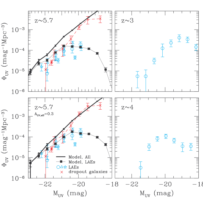
The thick solid curve in the top-left panel of Figure 16 is the UV LF for all sources (galaxies) in our model. Because of the tight correlation between SFR and halo mass, the curve is basically a transformation of the halo mass function with a constant mass-to-light ratio. This UV LF is from all the galaxies in our model, regardless of the apparent Ly$\alpha$ luminosity. To be detected as LAEs, the apparent Ly$\alpha$ luminosity should be high, which imposes a selection function onto the full UV LF. The UV LF of LAEs is from sources with apparent Ly$\alpha$ luminosity above a threshold, which is set in our model such that the number density of the selected LAEs (that can be observed) matches that of the $z=5.7$ LAEs in SXDS (about $4.0\times 10^{-4}{\rm Mpc}^{-3}$ for our adopted cosmology). The filled squares connected by thin solid curve shows the UV LF for the LAEs selected this way. For a cut in apparent Ly$\alpha$ luminosity, sources with a higher intrinsic Ly$\alpha$ luminosity (hence a higher UV luminosity) have a higher possibility to be selected (see Fig.8). As a result, the UV LF of LAEs is close to the full UV LF at the high luminosity end. However, in lower mass halos (sources with lower UV luminosity), fewer sources can have apparent Ly$\alpha$ luminosity high enough to be detected. The UV LF of LAEs becomes lower than the full UV LF. The ratio of the UV LFs of LAEs and all galaxies as a function of UV luminosity is nothing more than a reflection of the distribution of apparent Ly$\alpha$ luminosity as a function of halo mass (Fig.8). As a consequence of this simple effect, the UV LF of LAEs becomes flattened as the UV luminosity decreases and drops rapidly towards the low luminosity end (Fig.16).

The predicted features in the UV LF of LAEs are indeed seen in observations. The cyan points are observed UV LFs of $z=5.7$ LAEs (Shimasaku et al. 2006; Hu et al. 2006; Ouchi et al. 2008). The LF becomes flat for $M_{\rm UV}>-20.5$. The $z=5.7$ observations are not deep enough to show the predicted drop of the UV LF at the faint end, but the drop can be clearly seen in the $z\sim 3$ and $z\sim 4$ data, as shown in the right panels of Fig.16 (also see Fig.22 of Ouchi et al. 2008). Without any adjustment, the UV LF of LAEs from our model is in quite a reasonable agreement with observations. The observed flattening of the LF toward lower luminosity is well explained by our model. The agreement improves by adding an effective UV extinction of $A_{\rm UV,eff}=0.3$ to our model curve (lower left panel of Fig.16). As implied in § 6.1, the assumed IMF and the adopted SFR in the simulation may not be accurate, and we may need a higher UV luminosity. Therefore, the effective UV extinction here should be understood as a combination of the model uncertainty and dust extinction.

Kobayashi et al. (2010) present an LAE model with Ly$\alpha$ escape fraction and UV extinction being functions of metal column density and starforming and outflow phases of galaxies, which roughly reproduce the observed UV LF. The semi-analytic model of (Samui et al., 2009) with constant Ly$\alpha$ escape fraction and UV extinction fails to reproduce the turnover of the UV LF towards low luminosity end. By contrast, there is no Ly$\alpha$ escape fraction parameter and mass dependent UV extinction in our model, and the radiative transfer is the single factor responsible to convert the intrinsic Ly$\alpha$ emission to the observed one. In other words, the Ly$\alpha$ escape fraction, defined as the ratio of apparent to intrinsic Ly$\alpha$ luminosity is an output of the model. It is encouraging that our model, by accounting for simple physics, is able to reproduce the features in the observed UV LF. This is an independent output of our model and clearly lends credence to our model.

The sources that are not detectable as LAEs because of a low apparent Ly$\alpha$ luminosity can be detected as galaxies through the dropout technique (e.g., Bouwens et al., 2003). In Figure 16, the observed UV LF of the $z\sim 6$ $i$-dropout galaxies is shown as red crosses (Bouwens et al., 2006) and asterisk (Shimasaku et al., 2006). At the faint end, it agrees with the full UV LF from our model. It falls slightly steeper than our model curve at the bright end. Note that the $i$–dropout technique can miss LAEs with strong Ly$\alpha$ emission (Ouchi et al., 2008). The face values of UV LFs from our model and the data suggest that the sum of UV LFs of LAEs and dropout galaxies makes the full UV LF. Obviously, the sum should not double-count those LAEs that are also detected as dropout galaxies. Observations show that about 30–50% of dropout galaxies are detected as LAEs (e.g., Dow-Hygelund et al., 2007; Stanway et al., 2007; Ouchi et al., 2008) (our model implies that this fraction can depend on UV luminosity). Roughly accounting for this fraction, the nonduplicated sum of the observed UV LFs of LAEs and $i$–dropout galaxies seems to be in a reasonable agreement with the full UV LF from the model. This is yet another independent output of our model that agrees with observations.

We see that, as a consequence of Ly$\alpha$ radiative transfer, LAEs are sources that have a strong Ly$\alpha$ selection imposed. This selection effect nicely explains the shape of the observed UV LF of LAEs and that of the dropout galaxies.

6.3. Distribution of Ly$\alpha$ Equivalent Width

Figure 17.— Distribution of rest-frame Ly$\alpha$ equivalent width (EW₀) from the model. Different line types correspond to different UV magnitude.

Figure 18.— Rest-frame Ly$\alpha$ equivalent width (EW₀) as a function of UV luminosity. In both panels, the thick solid curve corresponds to the threshold of the observed (apparent) Ly$\alpha$ luminosity for the $z\sim 5.7$ LAEs in Ouchi et al. (2008), and the thick dashed vertical line shows the 3–$\sigma$ limit for the UV photometry in Ouchi et al. (2008). Dotted curves in both panels show the distribution of objects in the plane of EW₀ and UV luminosity from our model (see text): in the left panel, the contours denote the probability density of objects in the plane (thicker contours for higher densities); in the right panel, we plot the median (thin solid curve) and quartiles (dotted curves) of EW₀ for the LAEs that can be detected in Ouchi et al. (2008), i.e., for sources above the thick solid curve. The data points in both panels are taken from Ouchi et al. (2008): the filled circles and squares are for $z\sim 5.7$ LAEs in Ouchi et al. (2008) and Shimasaku et al. (2006) from the Subaru fields; the stars and diamonds represent $z\sim 6$ dropout galaxies in Stanway et al. (2007) and those compiled by Ando et al. (2006); the crosses denote $z\sim 5$ dropout galaxies in Ando et al. (2006).

As shown in the above two subsections, with simple assumptions to account for the model uncertainty, the model is able to reproduce the Ly$\alpha$ LF and UV LF of LAEs. We can go beyond the two LFs to study the joint distribution of Ly$\alpha$ and UV luminosities, which can be casted as the distribution of rest-frame Ly$\alpha$ EW as a function of UV luminosity. This distribution is not limited to LAEs and it can include that from the dropout galaxies.

Observationally, it is found that $z\sim 6$ galaxies seem to show a deficit of large EW values for UV luminous objects (Ando et al., 2006; Shimasaku et al., 2006; Stanway et al., 2007; Ouchi et al., 2008) (see the data points in Fig. 18). The threshold UV luminosity for the deficiency is $M_{\rm UV}=-21.5$ to -21.0 (Ando et al., 2006). Similar trend is seen for $z\sim$3–5 LAEs as well (e.g., Ouchi et al., 2008; Shioya et al., 2009). The trend is also reported for dropout galaxies at different redshifts (e.g., Shapley et al., 2003; Ando et al., 2007; Kajino et al., 2009; Pentericci et al., 2009; Vanzella et al., 2009). Ando et al. (2006) and other authors invoked the differences in dust extinction, amount of internal and surrounding neutral hydrogen gas, age of stellar population, and/or gas kinematics between UV faint and luminous galaxies as possible causes of the trend seen in Ly$\alpha$ EW and UV luminosity. Mao et al. (2007) present a model of high redshift galaxies including chemical evolution and dust attenuation. Kobayashi et al. (2010) also present a semi-analytic model of LAEs, in which Ly$\alpha$ and UV are attenuated differently by clumpy dust distribution. Both models seem to explain the deficiency of high Ly$\alpha$ EW in luminous galaxies essentially by means of halo mass dependent dust content. On the other hand, based upon a pure statistical analysis with $z\sim 3$ galaxies, Nilsson et al. (2009) conclude that there is no dependence of Ly$\alpha$ EW on UV luminosity for LAEs and Lyman break galaxies (LBGs). They interpret the lack of large Ly$\alpha$ EW, UV bright galaxies as an observational effect of small survey volumes.

For the model presented in this paper, the UV luminosity is directly related to halo mass and the apparent Ly$\alpha$ luminosity is determined by radiative transfer, which depends on the environment of galaxies (§ 7). It is interesting to see to what extent the observed relation between Ly$\alpha$ EW and UV luminosity can be explained by our model. Following § 6.1 and § 6.2, we scale the Ly$\alpha$ luminosity by a factor of 5 and apply an effective UV extinction of 0.3 for the UV luminosity for each LAE source.

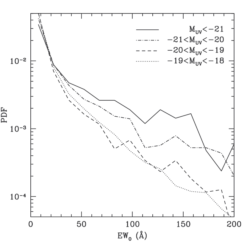
In our model, the intrinsic Ly$\alpha$ EW is a constant for all sources, since both the intrinsic Ly$\alpha$ luminosity and the UV luminosity are proportional to the SFR. Radiative transfer, however, gives rise to a broad distribution of the apparent (observed) Ly$\alpha$ EW. The distribution of the apparent EW is similar to that in Figure 8$b$, if the horizontal axis is relabeled. Figure 8$b$ shows the distribution in logarithmic space, while EW distribution in linear space matches more closely with what can be inferred from observations. In Figure 17, we show the distribution of rest-frame Ly$\alpha$ EW in linear space from our model. At a given UV luminosity, the distribution function of apparent Ly$\alpha$ EW is a decreasing function of EW. In the UV luminosity range considered here, the distribution function drops faster for sources with lower UV luminosity.

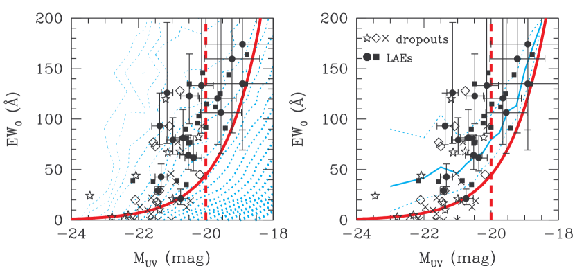
In the left panel of Figure 18, the cyan contours show the probability density distribution of objects in the plane of Ly$\alpha$ EW and UV luminosity from the model (thicker contours for higher densities). The apparent Ly$\alpha$ EW distribution at a fixed UV luminosity roughly follows an exponential distribution from our model, with fewer sources having larger EW. If the EW distribution did not vary with UV luminosity, the contour of equal probability density in the left panel of Figure 18 would appear to tilt along the direction of low EW and UV bright to high EW and UV faint because the number density of objects drops fast with UV luminosity. In our model, the apparent EW distribution has a weak dependence on UV luminosity, but it only leads to a slight change in tilt direction of the contour and cannot mask the effect caused by the decreasing number density toward high UV luminosity. The cyan contours in the left panel of Figure 18 clearly show that sources at the corner of large apparent EW and high UV luminosity have a low probability density. The low probability is a consequence of the combination of two facts: that UV LF drops steeply towards high luminosity and that the distribution of the apparent Ly$\alpha$ EW at fixed UV luminosity is a decreasing function of EW. The result suggests that a large survey volume is needed to discover large EW, UV bright sources, which is consistent with the conclusion in Nilsson et al. (2009). We note that we do not assume any particular form of the EW distribution at a given UV luminosity. In our model, we have a single value of intrinsic EW for all sources, since both intrinsic Ly$\alpha$ luminosity and UV luminosity are proportional to SFR and we apply the same scaling in either luminosity for all sources. The distribution of the apparent EW simply results from the radiative transfer effect.

Figure 19.— Distribution of Ly$\alpha$ rest-frame equivalent width (EW₀) for $z\sim 5.7$ LAEs. The dashed curve and the dotted histogram are two estimates of the distribution for all the photometrically selected $z\sim 5.7$ LAEs in Ouchi et al. (2008). The dashed curve is estimated from a maximum likelihood method by fully accounting for the probability distribution of the measured EW₀ for each LAE and the dotted histogram is obtained by simply adopting the best measurement of EW₀ (see Ouchi et al. 2008). The solid histogram is from our model for the corresponding population of LAEs, i.e., for LAEs that have the same number density as in Ouchi et al. (2008).

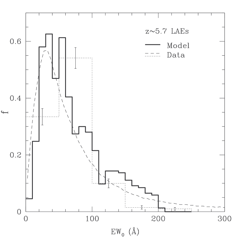
Because of the flux limit, luminosities of observed LAEs are above a threshold. The red solid curve in either panel of Figure 18 is the corresponding threshold for EW as a function of UV luminosity for $z=5.7$ LAEs in SXDS. To make a further comparison between the model and the observed LAEs, we show in the right panel of Figure 18 the median and quartiles (solid and dotted cyan curves) of the EW distribution as a function of UV luminosity from the model, for LAEs corresponding to those observed in the Subaru fields (filled circles and squares). The model prediction largely follows the observational trend. Again the lack of large EW, UV bright LAEs is evident in the model. Although the small number of observed LAEs prevents a comparison of the model and observed EW distribution as a function of UV luminosity, we can make a comparison for the overall EW distribution of the observed LAEs. The dashed curve and dotted histogram in Figure 19 are two estimates of the EW distribution for all the LAEs detected in SXDS inferred by Ouchi et al. (2008). The dashed curve is obtained with a maximum likelihood method by accounting for the full probability distribution of the measured EW for each LAE. The dotted histogram is obtained by simply counting the number of LAEs in each EW bin based on the measured values of EW, i.e., no uncertainty in the measured EW is assumed. According to Ouchi et al. (2008), the two estimates likely bracket the true distribution. The corresponding EW distribution from our model is shown as the solid histogram, which appears to be in good agreement with the observation estimates. Interestingly, it is more closely resemble the one from the maximum likelihood method.

Without appealing to differences in UV faint and UV bright sources, such as the amount of dust and age of stellar population, the observed deficit of bright UV galaxies with large Ly$\alpha$ EW is reproduced by the model. It is a natural consequence of the fact that UV LF drops toward high luminosity and the distribution of apparent EW at fixed UV luminosity is largely a decreasing function of EW. The model also reproduces the observed EW distribution. We emphasize that at fixed UV luminosity, the distribution of apparent EW in the model is completely determined by Ly$\alpha$ radiative transfer effect, not by any other mechanisms (e.g., different UV extinction or stellar age). Our model suggests that dependence of dust or stellar age on halo mass (or UV luminosity), if there is any, does not play a dominant role in the observed Ly$\alpha$ EW distribution of high-redshift galaxies and that Ly$\alpha$ radiative transfer is the main mechanism in determining the observational properties.

7. Important Physical Factors in Determining the Observability of LAEs

Figure 20.— Mean gas distribution profiles along the line of sight around halos of mass $8\times 10^{10}h^{-1}M_{\odot}$. In the left panels, from top to bottom, are temperature, neutral hydrogen density, and peculiar velocity profiles. Note that the halo velocity is subtracted from the peculiar velocity. The dotted curve in each panel is the mean profile for all the halos in the narrow mass bin around $8\times 10^{10}h^{-1}M_{\odot}$. The thin and thick solid curves are those in the lower and upper quartiles of the apparent to intrinsic Ly$\alpha$ luminosity ratio. In the corresponding panel on the right, we show the profile with respect to the mean profile, i.e., the mean profile for all halos in the mass bin is subtracted.

Figure 21.— Dependence of Ly$\alpha$ flux suppression of LAEs on density and peculiar velocity. The suppression is characterized by the ratio of the apparent (observed) and intrinsic Ly$\alpha$ luminosity $L_{\rm apparent}/L_{\rm intrinsic}$. Panel (a): dependence on the smoothed overdensity field at the source position. The overdensity field is smoothed with a 3D top-hat filter of radius 2$h^{-1}{\rm Mpc}$ (comoving), which is chosen to be larger than the size of the infall region around halos. Panel (b): dependence on the density gradient along the $Z$ direction. The derivative is with respect to comoving coordinate. Panel (c): dependence on the host halo velocity. Panel (d): dependence on the linear peculiar velocity gradient along the $Z$–direction. The linear peculiar velocity is obtained from the smoothed overdensity field based on the continuity equation (see text for detail). The velocity gradient is put in units of the Hubble parameter. In each panel, the solid curve is the median ratio and the two dotted curves delineate the upper and the lower quartiles. Note that the observation is along the $-Z$ direction, which matters for interpreting the results in of panels ($b$) and ($c$). See the text.

In previous sections, we study statistical properties of Ly$\alpha$ emission of LAEs in our model. At a fixed intrinsic Ly$\alpha$ luminosity, the apparent luminosity and peak wavelength shift have broad distributions. The cause of the distribution must be related to the underlying distribution and kinematics of gas, hence the matter distribution, around LAE sources, since Ly$\alpha$ radiative transfer is sensitive to the density and velocity fields. In this section, we study the correlations between the apparent Ly$\alpha$ properties and the environment of matter around sources. By revealing the physical causes, such correlations would aid our understanding of the observability and the statistical properties of LAEs.

To identify the key factors in shaping the observability of LAEs, we first choose LAE host halos in a narrow mass bin ($\sim 8\times 10^{10}h^{-1}M_{\odot}$) and stack the neutral gas density, temperature, and peculiar velocity profiles along the line of sight centered on these halos. As shown by the dotted curve in the middle-left panel of Figure 20, the stacked density profile around a halo appears to peak at the halo center and to be symmetric around the center. The central density is about a factor of 2000 higher than the mean cosmic density. We then stack only sources that are strongly and weakly suppressed in Ly$\alpha$ luminosity (e.g., the upper and lower quartiles of $L_{\rm apparent}/L_{\rm intrinsic}$), respectively, into two subsets. The stacked density profiles of strongly and weakly suppressed sources (thin and thick solid curves in the middle-left panel of Fig. 20) appear to have a relative offset in amplitude and are asymmetric in opposite directions. The trend becomes clear with the total mean profile subtracted (middle-right panel of Fig. 20). The temperature profiles of strongly and weakly suppressed Ly$\alpha$ sources also show systematic but small differences (top panels of Fig. 20). As temperature is largely linked to density inside halos, we tend to incorporate its effect into an overall density effect. The difference in amplitude and asymmetry of density profiles between strongly and weakly suppressed sources indicates that density and density gradient along the line of sight contribute to the observability of LAEs.

The overall stacked peculiar velocity profile around a halo (bottom-left panel of Fig. 20), with the velocity centered on the halo velocity, shows clear signatures of infall region: an inner Hubble-like contraction region near the center and an outer region with infall velocity decreasing outward. Similar to the density profile, we find difference in the slope of the velocity profile in the outer infall region between strongly and weakly suppressed Ly$\alpha$ sources (bottom-right panel of Fig. 20). Therefore, the peculiar velocity gradient along the line of sight is a factor in determining the observability of LAEs. We check the dependence on the line-of-sight velocity of halos and find that halo velocity also contributes to the LAE observability.

The above exercises provide us with the initial evidence on what physical variables affect the observability of LAEs. Since on scales larger than halo size, gas density and velocity largely follow those of the underlying dark matter, we identify the matter density and peculiar velocity and their gradients along the line of sight as the major factors in shaping the LAE observability. We proceed to study the correlation between these quantities and the suppression in Ly$\alpha$ luminosity for all the sources in our model. We are interested in the environment density and velocity around sources, not those inside halos, but they cannot be obtained directly at the positions of halos from the outputs of the reionization simulation. To eliminate the influence of density and velocity profiles inside halos, we smooth the density field with a 3D top-hat filter of radius of 2$h^{-1}{\rm Mpc}$ (comoving). Conclusions reached below are largely immune to possible uncertainties related to limited resolution of the hydro simulations we use ($\sim$65kpc comoving), which nonetheless is much smaller than 2$h^{-1}{\rm Mpc}$ comoving.

With the smoothed overdensity field $\delta$, we solve the linear peculiar velocity from the continuity equation

$$\dot{\delta}+\frac{1}{a}\nabla\cdot{\mathbf{v}}=0,$$ (6)

where $\dot{\delta}$ can be written as $fH(a)\delta$ with $f=d\ln\delta/d\ln a$ the derivative of the growth factor and $H(a)$ the Hubble parameter at the time when the scale factor is $a$. The peculiar velocity field is obtained from the Fourier transform

$${\mathbf{v}}=fHa\sum_{\mathbf{k}}\frac{ik_{z}}{k^{2}}\delta_{\mathbf{k}}e^{i{\mathbf{k}}\cdot{\mathbf{r}}},$$ (7)

where $\delta_{\mathbf{k}}$ is the Fourier transform of the smoothed overdensity field. The velocity gradient and density gradient along the $Z$ direction are

$$\frac{\partial v_{z}}{\partial z}=-fHa\sum_{\mathbf{k}}\frac{k_{z}^{2}}{k^{2}}\delta_{\mathbf{k}}e^{i{\mathbf{k}}{\mathbf{\cdot}}{\mathbf{r}}}$$ (8)

and

$$\frac{\partial\delta}{\partial z}=\sum_{\mathbf{k}}ik_{z}\delta_{\mathbf{k}}e^{i{\mathbf{k}}\cdot{\mathbf{r}}}.$$ (9)

The spatial derivatives in all the above equations are with respect to comoving coordinates.

Figure 21 shows the correlations of the apparent to intrinsic luminosity ratio with the environment overdensity, velocity and their gradient along the line of sight for all the LAEs in our model. The trends of correlations at a fixed halo mass look similar, with amplitudes and slopes of curves slowly evolving with mass. These correlations reflect different aspects of Ly$\alpha$ radiative transfer. In what follows, we interpret them in turn.

Figure 21$a$ shows that Ly$\alpha$ emission from LAEs is more strongly suppressed in denser region. This seems easy to understand — higher density means high optical depth for Ly$\alpha$ emission. At the high end of the density, high optical depth also leads to large Ly$\alpha$ frequency diffusion (and more spatial diffusion), which appears to be able to compensate for otherwise reduced Ly$\alpha$ transmission due to high optical depth. As a result, the curve of the overall luminosity suppression factor flattens at very high density. In details, the above understanding is not complete. Through the continuity equation (eq.[6]), density is anti-correlated with velocity gradient. As shown below (Fig. 21$d$), velocity gradient plays a dominant role in determining the suppression factor. As will be elaborated in Paper II, the density dependence seen here is largely driven by its anti-correlation with the velocity gradients, while velocity gradients along different directions contributes a lot to the anisotropic Ly$\alpha$ emission distribution.

Figure 21$b$ shows that Ly$\alpha$ sources are easier to be transmitted if the local density has a negative gradient along the line of sight, i.e., density decreases towards the observer. Note that the observation direction (line of sight) for Ly$\alpha$ emission in our radiative transfer modeling is set to be along the $-Z$ direction, therefore negative gradient means that sources are located on the near side of overdense regions or on the far side of underdense regions. With respect to sources located on the far side of overdense regions or on the near side of underdense regions, Ly$\alpha$ photons encounter a decreasing density profile, thus low optical depth, along their way to the observer. Although these photons also travel across other overdense and underdense regions, the redshifting of these photons caused by Hubble expansion would make these intervening regions largely transparent to them. That is, only the immediate environments of the sources affect their observability.

Figure 21$c$ show that, with respect to the Hubble flow, LAEs moving away from the observer have a lower suppression in Ly$\alpha$ luminosity than those moving towards the observer. Note that sources with negative velocities are the ones moving away from the observer, since we observe along the $-Z$ direction. The IGM on scales larger than LAE host halos can detach from the motion of halos to some degree, and experiencing Hubble expansion. The motion of the halo with respect to the surrounding IGM thus introduces a dipole in the Ly$\alpha$ optical depth around the source. For sources moving away from the observer, Ly$\alpha$ photons acquire an additional redshift from the halo motion, and hence the direction towards the observer is the one that has the lower optical depth and photons preferentially “leak” towards that direction.

Figure 21$d$ shows that the line-of-sight gradient of the line-of-sight velocity has the largest effect in shaping the LAE observability. We see that sources located at places that have larger line-of-sight gradient in peculiar velocity are easier to be observed. A local velocity gradient effectively changes the local Hubble expansion rate. A positive gradient increases the local expansion rate. A faster expansion makes Ly$\alpha$ photons on the red side of line center much easier to escape. It also makes Ly$\alpha$ photons on the blue side of line center travel a shorter distance to redshift to the line center and to be scattered in the IGM, and therefore the escaping photons after frequency diffusion are more centrally distributed, leading to higher surface brightness. Both of these effects cause the transmission of Ly$\alpha$ photons that is enhanced for sources with positive local velocity gradient.

We see that the major factors in determining LAE observability all have clear physical origins. Quantities like the density gradient, velocity, and velocity gradient are statistically interrelated. For example, in a statistical sense, sources on the near side of an overdense region (negative density gradient) usually moving away from us (negative velocity). However, on a source by source basis, because of the randomness of the density and velocity field, this is not always true. In other words, there are large scatters among the correlations of these quantities. Since these different quantities have different physical effects on Ly$\alpha$ transmission, the overall Ly$\alpha$ transmission or luminosity suppression effect should be a supposition of all of them.

The dependence of Ly$\alpha$ radiative transfer on large scale density and peculiar velocity fields imposes a strong selection effect on observations of LAEs. The selection leads to new features in the clustering of LAEs, which are investigated in Paper II.

Some of the environment factors identified here are expected to be found in the $\exp(-\tau_{\nu})$ model. For example, Iliev et al. (2008) compare the results from the $\exp(-\tau_{\nu})$ model with and without the peculiar velocity field turning off. They find that both the gas infall around halos and source peculiar velocity are important in determining the suppression factors of Ly$\alpha$ luminosity and in shaping the observed Ly$\alpha$ luminosity, especially at the luminous end (see their Figures 21, 23 and 24). This is qualitatively in parallel with our finding that source peculiar velocity and peculiar velocity gradient of surrounding matter are important factors. While McQuinn et al. (2007) consider the cases of varying the global neutral fraction, which shows the effect of density on the suppression of Ly$\alpha$ luminosity, it is clearly different from what we intend to do here. Nevertheless, we expect that the density and density gradient effects also show up in the $\exp(-\tau_{\nu})$ model, given that they contribute to the line-of-sight optical depth. Although in most cases the simple $\exp(-\tau_{\nu})$ model can provide qualitative understanding of Ly$\alpha$ radiative transfer results, we do not expect it to capture all the physics. In the $\exp(-\tau_{\nu})$ model, the radiative transfer is completely determined by the line-of-sight optical depth. In the full calculation, this is not the case – the scatterings of Ly$\alpha$ photons enable them to probe the optical depth in all directions and the line-of-sight outcome depends on not only the line-of-sight optical depth but also those in other directions (see more details in Paper II).

8. Summary and Discussion

8.1. Summary of Main Results

We perform a full Ly$\alpha$ radiative transfer calculation with a Monte Carlo code (Zheng & Miralda-Escudé, 2002) to study LAEs in a cosmological volume. The LAE sources and the physical properties of neutral hydrogen gas are taken from the $z\sim 5.7$ outputs of a cosmological reionization simulation (Trac et al., 2008), which solves the coupled evolution of the dark matter, baryons, and ionizing radiation in a box of 100$h^{-1}{\rm Mpc}$ (comoving) on a side. The large volume of the simulation allows a statistical study of $z\sim 5.7$ LAEs. Radiative transfer of Ly$\alpha$ photons in the IGM environment around LAEs, which leads to both frequency and spatial diffusion of Ly$\alpha$ photons, turns out to play a crucial role in determining the observability of LAEs and in understanding the observed properties of LAEs.

Although the radiative transfer calculation is computationally costly, the LAE model we present in this paper is rather simple. The UV or intrinsic Ly$\alpha$ luminosity is assumed to be proportional to the SFR, which is tightly coupled to halo mass in the reionization simulation we use. That is, we essentially adopt a constant mass to light ratio, where mass is halo mass and light is either UV or Ly$\alpha$ . All we do is to add the physics of Ly$\alpha$ radiative transfer into the model to obtain the observed properties of LAEs. That is, we introduce the radiative transfer of Ly$\alpha$ photons in the IGM as the single factor responsible for transforming the intrinsic Ly$\alpha$ emission properties to the observed ones. Our model produces IFU-like data cube that covers the extent of the simulation box, which allows mock observations to be made. With the Ly$\alpha$ image contracted from this data cube, we follow typical observational procedures (e.g., Ouchi et al., 2008) to identify LAEs and then extract their Ly$\alpha$ spectra.

Initially Ly$\alpha$ photons are produced inside the star formation region. Therefore the intrinsic Ly$\alpha$ sources are expected to be similar in size as the UV sources, which are compact ($\lesssim 1$ kpc; Taniguchi et al. 2009). We find that an intrinsically point-like Ly$\alpha$ source becomes extended as a consequence of resonant scatterings of Ly$\alpha$ photons (spatial diffusion). The scatterings of Ly$\alpha$ photons do not destroy them and all Ly$\alpha$ photons escape in the end. However, observationally, only the central part of the extended source can be detected as a consequence of the limit set by the surface brightness threshold. The scatterings of Ly$\alpha$ photons also cause the frequency of Ly$\alpha$ photons to change (frequency diffusion). The resultant Ly$\alpha$ spectra from the central aperture do not have a simple relation to the initial profile, which is assumed to be Gaussian in our model. Our results from full radiative transfer calculations show a clear difference from a simple treatment of Ly$\alpha$ radiative transfer, namely the $\exp(-\tau_{\nu})$ model, widely adopted in previous work, which modifies the intrinsic Ly$\alpha$ spectrum by multiplying the line-of-sight transmission determined by the optical depth at each frequency.

The observed Ly$\alpha$ spectrum of an LAE in our model shows a clear asymmetry, skewed towards red. Although the $\exp(-\tau_{\nu})$ model produces the same qualitative feature, the predicted line profile, the frequency shift, and the total flux are all significantly different from our results. While the spectrum of the $\exp(-\tau_{\nu})$ model we present is essentially the intrinsic one truncated below a certain wavelength (but see Figures 14 and 15 in Iliev et al. 2008 for more complex line shapes, probably caused by different assumptions in the $\exp(-\tau_{\nu})$ model), the observed Ly$\alpha$ spectrum in our model can have contributions from photons with frequency much redder than initial photons, a result of the scattering-caused frequency diffusion. We find that the redward shift of the Lya line induced by radiative transfer is usually a few times the intrinsic line width, with a distribution that peaks at about three times. The asymmetry and shift of the Ly$\alpha$ line do not indicate the presence of any winds, but they arise from the structure of the halo infall and Hubble expansion around the sources. If one were to infer the wind velocity, if there is any, from comparing the relative shift in the Ly$\alpha$ line and an optically-thin line, one has to keep in mind the Ly$\alpha$ radiative transfer effect. For example, the observationally inferred velocity of the receding winds would be overestimated by $\sim 100{\rm km\,s^{-1}}$ or more if the effect is not taken into account.

As a consequence of the frequency diffusion and spatial diffusion, our model predicts a much higher observed Ly$\alpha$ flux than the $\exp(-\tau_{\nu})$ model. At a fixed intrinsic Ly$\alpha$ luminosity (i.e., fixed host halo mass), the observed (apparent) luminosity is broadly distributed. The shift in the Ly$\alpha$ line peak and the ratio of the apparent to intrinsic Ly$\alpha$ luminosity appear to be anti-correlated. The distributions of the line peak shift and the ratio of apparent to intrinsic Ly$\alpha$ luminosity, and their correlation, all result from the dependence of the Ly$\alpha$ radiative transfer on the IGM environments around sources. It would be interesting and extremely useful if we could make use of the full information in the observed Ly$\alpha$ properties to infer the intrinsic ones, and we reserve such an investigation for future work. Although our model predicts a much higher observed Ly$\alpha$ flux than the $\exp(-\tau_{\nu})$ model, it still leads to a highly suppressed Ly$\alpha$ flux, compared with the intrinsic one. The suppression factor depends on the assumed line width of the intrinsic Ly$\alpha$ spectra. For the line width assumed in our model (given by halo virial temperature), we find that, with respect to the intrinsic Ly$\alpha$ LF of LAEs, the observed (apparent) Ly$\alpha$ LF shift towards the low luminosity end by roughly one order of magnitude in luminosity. For comparison, the $\exp(-\tau_{\nu})$ model would shift by two orders of magnitude in luminosity.

We make comparisons between the $z\sim 5.7$ LAEs in our model and those observed in SXDS (Ouchi et al., 2008). The sizes, morphologies, Ly$\alpha$ line profiles of the model LAEs are remarkably similar to the observed ones. For the Ly$\alpha$ LF, UV LF, and Ly$\alpha$ EW distribution, our model can successfully reproduce the observations and provide physical explanations for various observed features.

After an overall adjustment of a factor of $\sim 5$ in luminosity, the Ly$\alpha$ LF of model LAEs matches well with observation. The adjustment reflects our incomplete knowledge in the stellar IMF at high redshift, the uncertainty in the model SFR, and the lack of information on the intrinsic Ly$\alpha$ line profile. According to our model, there is no one-to-one map between the intrinsic and the observed Ly$\alpha$ luminosity. In other words, there is a large scatter in the relation between the apparent and intrinsic luminosities. At a fixed observed luminosity, LAEs can differ by one order of magnitude in the intrinsic luminosity (Fig. 8$c$). This large scatter has to be taken into account when interpreting the observed Ly$\alpha$ LF and linking the observed LAEs to their host halos.

For the UV LF of observed LAEs, our model prediction shows a good agreement with observation. In particular, the turnover of the UV LF towards the low luminosity end seen in high-$z$ ($z\sim$ 3–6) LAEs are well reproduced. The key to interpret the shape of the UV LF is that observed LAEs are sources with observed (apparent) Ly$\alpha$ luminosity above certain threshold. The turnover reflects that for LAEs with low UV luminosity (or low intrinsic Ly$\alpha$ luminosity, or low halo mass), the probability for the observed Ly$\alpha$ luminosity to exceed the observation threshold is low, a consequence of the broad distribution of apparent Ly$\alpha$ luminosity at a given intrinsic Ly$\alpha$ luminosity. The full UV LF for sources in our model (i.e., without imposing the observation Ly$\alpha$ luminosity threshold) agrees well with the nonduplicated sum of the observed UV LFs of LAEs and $i$–dropout galaxies at $z\sim 6$.

The observed distribution of Ly$\alpha$ EW as a function of UV luminosity is also reproduced in the model. We note that in our model all the sources have the same intrinsic EW and the distribution of the observed values of EW at fixed UV luminosity is purely caused by the environment-dependent radiative transfer effect. At a fixed UV luminosity, the distribution of observed (apparent) EW is a decreasing function toward high values. The observational trend of lacking UV bright, high EW sources (e.g., Ando et al., 2006) is naturally explained by our model in that such sources lie in a low probability corner — a combination of the drop of the UV LF toward high luminosity and the drop of the apparent EW distribution function toward high EW value. LAE surveys with large volume will test the interpretation.

Therefore, the observed properties of LAEs can be explained by simply invoking Ly$\alpha$ radiative transfer: the effects of the local IGM environment, depending mainly on the gas density and line-of-sight velocity and their line-of-sight gradients, lead to the distribution of observed Ly$\alpha$ emission properties at fixed intrinsic Ly$\alpha$ luminosity. This environmental selection also causes new features in the clustering of LAEs that we will study in Paper II.

8.2. Implications and Discussion

Our interpretation of the observations of LAEs does not invoke any mass dependent dust absorption, which is in contrast to many previous models (e.g., Dayal et al., 2010). Uniformly distributed dust efficiently absorbs Ly$\alpha$ photons, since the large number of resonant scatterings increase the path length. There is much less attenuation when the dust is in gas clumps and Ly$\alpha$ photons bounce off the cloud surfaces (Neufeld, 1991; Hansen & Oh, 2006). Optical, UV, and Ly$\alpha$ observations of local star-forming galaxies provide evidence that ISM kinematics and geometry play a more significant role than dust in affecting the Ly$\alpha$ emission (e.g., Giavalisco et al., 1996; Keel, 2005; Atek et al., 2008, 2009). Our model successfully reproduces the observed UV LF of LAEs by incorporating only a mass independent effective UV extinction of at most 0.3 mag. We conclude that any mass dependent dust effects are not likely to play a substantial role to determine the observed properties of LAEs, compared to Ly$\alpha$ radiative transfer effects.

Our model also has important implications for the duty cycle and the Ly$\alpha$ escape fraction of LAEs. The theoretically predicted (intrinsic) Ly$\alpha$ LF, which essentially is the halo mass function, is substantially higher than the observed one. Two scenarios have been introduced to address this problem, the duty cycle and the Ly$\alpha$ escape fraction scenarios (e.g., Stark et al., 2007b; Nagamine et al., 2008). In the duty cycle scenario, LAEs are short-lived and a fraction of all galaxies are active as LAEs at any given time, lowering the amplitude of the Ly$\alpha$ LF. In the Ly$\alpha$ escape fraction scenario, only a fixed fraction of Ly$\alpha$ photons escape from the source and the overprediction problem is solved by shifting the LF towards the low luminosity end. To conserve the number density of LAEs of a given sample, the masses of host halos in the duty cycle scenario would be on average lower than those in the escape fraction scenario. As a consequence, the clustering of LAEs would be different in the two scenarios, with a stronger clustering in the escape fraction scenario. Nagamine et al. (2008) find that LAE clustering measurements from observations are in favor of their duty cycle scenario.

In our model, Ly$\alpha$ photons all escape after a large number of scatterings. The Ly$\alpha$ escape fraction, in its literal meaning, is therefore unity. However, only the central part of the extended Ly$\alpha$ emission of LAEs can be observed, which gives rise to an apparent or effective Ly$\alpha$ escape fraction. Since the observed Ly$\alpha$ luminosity has a broad distribution at a fixed intrinsic Ly$\alpha$ luminosity, our model predicts a broad distribution of the effective Ly$\alpha$ escape fraction rather than a single value. In our model, no duty cycle parameter is introduced. Since halos of the same mass have similar SFR in our model, the corresponding intrinsic Ly$\alpha$ luminosities are the same, i.e., Ly$\alpha$ emission does not come from a fraction of halos. However, an apparent or effective duty cycle arises as a result of the selection effect caused by Ly$\alpha$ radiative transfer (a broad distribution of observed Ly$\alpha$ luminosity at a fixed intrinsic Ly$\alpha$ luminosity) and a Ly$\alpha$ luminosity threshold in observation. This can be seen from comparing the UV LF for all galaxies (dropout galaxies and LAEs) and that for LAEs (Fig. 16), which can be described as that at a fixed UV luminosity (or halo mass) only a fraction of all the galaxies are observed as LAEs. This effective duty cycle does not have the physical meaning in its original form. Moreover, it is not a constant, since it changes with UV luminosity (Fig. 16). Tilvi et al. (2009) present an LAE model in which Ly$\alpha$ luminosity (or SFR) is related to the halo mass accretion rate, rather than halo mass, and the model naturally gives rise to the duty cycle of LAEs. The duty cycle in their model, however, has its original meaning, in direct contrast with our model. Our model still ties the intrinsic Ly$\alpha$ luminosity (SFR) to halo mass and let the Ly$\alpha$ radiative transfer do the work of converting it to observed Ly$\alpha$ luminosity. Because of the large scatter between the observed Ly$\alpha$ luminosity and the intrinsic one (or halo mass) in our model, for a sample of LAEs above a Ly$\alpha$ luminosity threshold, some of them can reside in halos with mass smaller than the threshold mass above which halos have the same number density as LAEs. So the effective duty cycle in our model has the effect of lowering the clustering amplitude of LAEs.

The main uncertainties in our model are the stellar IMF, the SFR, and the intrinsic Ly$\alpha$ line profile. The first two are general uncertainties for any model. The IMF at high-$z$ is neither well constrained observationally nor well understood theoretically. The SFR in galaxy formation model is related to the complex gas physics that we do not have a satisfactory understanding. Changing IMF or SFR would change the details in the reionization process and therefore change the gas properties (e.g., neutral fraction and temperature distribution) at a fixed redshift. For the reionization history itself, the escape fraction of ionizing photons adds a further uncertainty. Even though we focus on LAEs at $z\sim 5.7$, when reionization is almost complete, different reionization histories can still leave different imprints on the gas distribution. For example, the IGM temperature in a region is correlated to the time when this region is reionized and heated (e.g., Trac et al., 2008). A detailed study is needed to investigate the effect of inhomogeneous IGM temperature distribution on Ly$\alpha$ radiative transfer. To be fully self-consistent, for any change in the IMF, SFR, and escape fraction of ionizing photons, one has to re-run the reionization simulation to solve the density, velocity, and temperature distributions of neutral gas and then perform the Ly$\alpha$ radiative transfer calculation. If the IMF, SFR, and escape fraction of ionizing photons change in a way to maintain the same reionization history, the effect of the IMF and SFR change can be largely characterized by an overall scaling in UV or intrinsic Ly$\alpha$ luminosity and one does not need to redo the Ly$\alpha$ radiative transfer calculation. For simplicity and to avoid extensive computations for reionization and radiative transfer simulation, we adopt such a scenario in this paper. Changing the width of the intrinsic Ly$\alpha$ line profile leads to changes in the distribution of the apparent to intrinsic Ly$\alpha$ luminosity ratio. Although we cast the effect as an overall scaling in the apparent Ly$\alpha$ luminosity for the Ly$\alpha$ LF, the intrinsic Ly$\alpha$ line profile is important in many aspects of the Ly$\alpha$ observation (image, spectra, etc) and its effect deserves a detailed investigation. Ly$\alpha$ radiative transfer calculation with high resolution hydrodynamic simulations for individual LAEs are necessary to shed light on the intrinsic Ly$\alpha$ line profile (e.g., Laursen & Sommer-Larsen, 2007). Changing the IMF affects the flux of ionizing photons more than that of the $\sim$ 1500ÅUV photons, which leads to a change in the ratio of the intrinsic Ly$\alpha$ luminosity to UV luminosity, or the intrinsic Ly$\alpha$ EW. Intrinsic Ly$\alpha$ line profile and dust play a role in converting the intrinsic EW to apparent EW, with the former affecting the Ly$\alpha$ luminosity and the latter adding extinction to UV luminosity. Therefore, the full distribution of observed Ly$\alpha$ EW and UV luminosity of LAEs can give constraints on the IMF, SFR, dust, and intrinsic Ly$\alpha$ profile.

Although we have identified key environment factors in shaping the observational properties of LAEs, the dependence of radiative transfer on environments deserves a further study to understand the details of Ly$\alpha$ scatterings in the surrounding regions of LAEs.

Our Ly$\alpha$ radiative transfer calculation relies on the gas distribution and properties from the cosmological reionization simulation. The radiative transfer of ionizing photons with a ray tracing algorithm is crucial in determining the state of gas. We have tested our LAE model for a reionization simulation with improved ray tracing algorithm (Trac et al. in prep.) in a small box (25$h^{-1}{\rm Mpc}$ on a side). We find that the results presented in this paper are robust.

Ly$\alpha$ radiative transfer through the surrounding circumgalactic and intergalactic media is a physical process that likely plays an important role in galaxies at all redshifts. It has to be taken into account for modeling LAEs and for interpreting observations. Our model is rather simple and can naturally explain an array of observations of LAEs, which make it extremely attractive. It is interesting to see how well it does in interpreting observations of LAEs at lower redshifts (e.g., $z\sim 3$). We also plan to apply it to the era of the late stage of reionization to study how to use LAEs to constrain reionization.

Appendix A Effects of the Initial Ly$\alpha$ Line Width and Gas Temperature in the $\exp(-\tau_{\nu})$ Model

Figure 22.— Effects of the initial Ly$\alpha$ line width and gas temperature in the $\exp(-\tau_{\nu})$ Model. Left panel: Ratio of the apparent (observed) to intrinsic Ly$\alpha$ luminosity as a function of the initial Ly$\alpha$ line width $\sigma_{\rm init}$. The bottom axis marks the line width in terms of the width $\sigma_{\rm vir}$ set by halo virial temperature, while the top axis in units of the circular velocity $v_{c}$ at halo virial radius. The thick and thin solid curves are the median and quartiles of the luminosity ratio distribution for the case using gas temperature in the reionization simulation. The set of dotted curves are the same but with the gas temperature set to $10^{4}$K in all regions. Right panel: Thermally averaged cross-section of Ly$\alpha$ scattering as a function of gas temperature. The bottom axis marks the frequency offset with respect to the Ly$\alpha$ line center and the top axis indicates the fluid velocity that can give rise to such an offset. The cross-section is composed of a thermal (Gaussian) core and a Lorentzian wing dominated at small and large frequency offsets, respectively. Changing gas temperature from $10^{5}$K to $10^{4}$K has a large effect on the Ly$\alpha$ scattering cross-section for gas with velocity in the range of $\sim$10–100${\rm km\,s^{-1}}$. See text for details.

In § 5, we make comparisons of the results from full radiative transfer calculation and those from the $\exp(-\tau_{\nu})$ model (see Figures 10–13). The $\exp(-\tau_{\nu})$ model has been widely adopted in studying LAEs. While the $\exp(-\tau_{\nu})$ model we present in this paper predicts that the apparent Ly$\alpha$ luminosity is at the level of a few percent of the intrinsic one, leading to large offset of the apparent Ly$\alpha$ luminosity function with respect to the one measured from observation, the $\exp(-\tau_{\nu})$ model in other work (e.g., McQuinn et al., 2007; Iliev et al., 2008) does not show such a large suppression in Ly$\alpha$ flux. For example, the apparent-to-intrinsic Ly$\alpha$ luminosity ratio is at the level of tens of percent for models in Iliev et al. (2008). The appendix aims at resolving the discrepancy by clarifying the assumptions adopted in our $\exp(-\tau_{\nu})$ model and others.

In our $\exp(-\tau_{\nu})$, we assume the same initial Ly$\alpha$ line width as with the full radiative transfer calculation. The initial rms line width is determined by the halo virial temperature (see § 3), $\sigma_{\rm init}=31.9[M_{h}/(10^{10}h^{-1}M_{\odot})]^{1/3}{\rm km\,s^{-1}}$. We also adopt the gas temperature provided by the reionization simulation, which is solved self-consistently in the simulation. As shown in Figure 20, the temperature of the gas drops from $\sim 10^{5}$K near the source center to $\sim 10^{4}$K in the IGM. For comparison, the initial line width and gas temperature adopted in other work are different from ours. For example, the fiducial model in McQuinn et al. (2007) adopt a line width set by the circular velocity at halo virial radius, which is about 2.3 times higher than our value. Iliev et al. (2008) assume the initial rms line width to be 160${\rm km\,s^{-1}}$ for all sources, which is much larger than the value we use for most sources. Both McQuinn et al. (2007) and Iliev et al. (2008) assume the gas temperature in all regions to be $10^{4}$K when computing the transmission of Ly$\alpha$ emission. Given these different assumptions used in our work and others, we perform tests of the effects of initial line width and gas temperature on the Ly$\alpha$ flux suppression in the $\exp(-\tau_{\nu})$ model with a small simulation (box size of 25$h^{-1}{\rm Mpc}$ on a side). We calculate the distribution of the apparent-to-intrinsic Ly$\alpha$ luminosity ratio for all sources with halo mass above $5\times 10^{9}h^{-1}M_{\odot}$.

The solid curves in the left panel of Figure 22 show the median and quartiles of the apparent-to-intrinsic Ly$\alpha$ luminosity ratio as a function of the initial line width for the case using gas temperature in the reionization simulation. The results presented in § 5 are based on the (default) value $\sigma_{\rm init}/\sigma_{\rm vir}=1$. As expected, the luminosity ratio is sensitive to the initial line width. At $\sigma_{\rm init}/\sigma_{\rm vir}=2$ the median ratio is about one order of magnitude higher than that from our default case.

The dotted curves in the left panel of Figure 22 correspond to the case with gas temperature set to $10^{4}$K in all regions. Changing the gas temperature leads to changes in the thermally averaged cross-section for Ly$\alpha$ scattering. As shown in the right panel of Figure 22, the scattering cross-section is composed of a thermal (Gaussian) core and a Lorentzian wing dominated at small and large frequency offsets, respectively. The core is wider at higher temperature. Since the temperature around a source in the reionization simulation can be higher than $10^{4}$K (Fig. 20), setting the temperature to $10^{4}$K would underestimate the scattering optical depth near the source and overestimate the transmitted flux. This explains why the luminosity ratio in the case with $T=10^{4}$K is higher than that with simulation temperature (left panel). For a quantitative comparison, we note that Iliev et al. (2008) present a case with $\sigma_{\rm init}/\sigma_{\rm vir}\simeq 2.2$ and $T=10^{4}$K (rightmost panel of their Fig.25) and the median luminosity ratio is $\sim$0.33. Under the same assumptions, our $\exp(-\tau_{\nu})$ model in Figure 22 gives a median ratio of $\sim$0.25, in broad agreement with their result. The residual difference may be caused by the difference in the simulations (e.g., hydrogen neutral fraction).

To conclude, the outcome of the $\exp(-\tau_{\nu})$ model depends on the initial Ly$\alpha$ line width and gas temperature distribution and our $\exp(-\tau_{\nu})$ model results are consistent with others if the same assumptions are adopted.

References

- Adams (1972) Adams, T. F. 1972, ApJ, 174, 439
- Adelberger et al. (2003) Adelberger, K. L., Steidel, C. C., Shapley, A. E., & Pettini, M. 2003, ApJ, 584, 45
- Ahn et al. (2000) Ahn, S.-H., Lee, H.-W., & Lee, H. M. 2000, Journal of Korean Astronomical Society, 33, 29
- Ahn et al. (2001) Ahn, S.-H., Lee, H.-W., & Lee, H.M. 2001, ApJ, 554, 604
- Ahn et al. (2002) Ahn, S.-H., Lee, H.-W., & Lee, H.M. 2002, ApJ, 567, 922
- Ando et al. (2006) Ando, M., Ohta, K., Iwata, I., Akiyama, M., Aoki, K., & Tamura, N. 2006, ApJ, 645, L9
- Ando et al. (2007) Ando, M., Ohta, K., Iwata, I., Akiyama, M., Aoki, K., & Tamura, N. 2007, PASJ, 59, 717
- Atek et al. (2008) Atek, H., Kunth, D., Hayes, M., Östlin, G., & Mas-Hesse, J. M. 2008, A&A, 488, 491
- Atek et al. (2009) Atek, H., Schaerer, D., & Kunth, D. 2009, A&A, 502, 791
- Auer (1968) Auer, L. H. 1968, ApJ, 153, 783
- Avery & House (1968) Avery, L. W., & House, L. L. 1968, ApJ, 152, 493
- Bouwens et al. (2003) Bouwens, R. J., et al. 2003, ApJ, 595, 589
- Bouwens et al. (2006) Bouwens, R. J., Illingworth, G. D., Blakeslee, J. P., & Franx, M. 2006, ApJ, 653, 53
- Chabrier (2003) Chabrier, G. 2003, PASP, 115, 763
- Cowie & Hu (1998) Cowie, L. L., & Hu, E. M. 1998, AJ, 115, 1319
- Cuby et al. (2007) Cuby, J.-G., Hibon, P., Lidman, C., Le Fèvre, O., Gilmozzi, R., Moorwood, A., & van der Werf, P. 2007, A&A, 461, 911
- Davé (2008) Davé, R. 2008, MNRAS, 385, 147
- Dayal et al. (2008) Dayal, P., Ferrara, A., & Gallerani, S. 2008, MNRAS, 389, 1683
- Dayal et al. (2009) Dayal, P., Ferrara, A., Saro, A., Salvaterra, R., Borgani, S., & Tornatore, L. 2009, MNRAS, 400, 2000
- Dayal et al. (2010) Dayal, P., Maselli, A., & Ferrara, A. 2010, arXiv:1002.0839
- Dey et al. (1998) Dey, A., Spinrad, H., Stern, D., Graham, J. R., & Chaffee, F. H. 1998, ApJ, 498, L93
- Dijkstra et al. (2006) Dijkstra, M., Haiman, Z., & Spaans, M. 2006, ApJ, 649, 14
- Dijkstra et al. (2007) Dijkstra, M., Lidz, A., & Wyithe, J. S. B. 2007, MNRAS, 377, 1175
- Dijkstra et al. (2007) Dijkstra, M., Wyithe, J. S. B., & Haiman, Z. 2007, MNRAS, 379, 253
- Dijkstra et al. (2006a) Dijkstra, M., Haiman, Z., & Spaans, M. 2006a, ApJ, 649, 14
- Dijkstra et al. (2006b) Dijkstra, M., Haiman, Z., & Spaans, M. 2006b, ApJ, 649, 37
- Dow-Hygelund et al. (2007) Dow-Hygelund, C. C., et al. 2007, ApJ, 660, 47
- Dunkley et al. (2009) Dunkley, J., et al. 2009, ApJS, 180, 306
- Eisenstein et al. (2005) Eisenstein, D. J., et al. 2005, ApJ, 633, 560
- Franx et al. (1997) Franx, M., Illingworth, G. D., Kelson, D. D., van Dokkum, P. G., & Tran, K.-V. 1997, ApJ, 486, L75
- Furlanetto et al. (2005) Furlanetto, S. R., Schaye, J., Springel, V., & Hernquist, L. 2005, ApJ, 622, 7
- Furlanetto et al. (2006) Furlanetto, S.R., Zaldarriaga, M., & Hernquist, L. 2006, MNRAS, 365, 1012
- Giavalisco et al. (1996) Giavalisco, M., Koratkar, A., & Calzetti, D. 1996, ApJ, 466, 831
- Haiman & Cen (2005) Haiman, Z., & Cen, R. 2005, ApJ, 623, 627
- Haiman & Spaans (1999) Haiman, Z., & Spaans, M. 1999, ApJ, 518, 138
- Hansen & Oh (2006) Hansen, M., & Oh, S. P. 2006, MNRAS, 367, 979
- Harrington (1973) Harrington, J. P. 1973, MNRAS, 162, 43
- Harrington (1974) Harrington, J. P. 1974, MNRAS, 166, 373
- Hill et al. (2008) Hill, G. J., et al. 2008, Astronomical Society of the Pacific Conference Series, 399, 115
- Horton et al. (2004) Horton, A., Parry, I., Bland-Hawthorn, J., Cianci, S., King, D., McMahon, R., & Medlen, S. 2004, Ground-based Instrumentation for Astronomy, ed. A.F. M. Moorwood and I. Masanori, Proceedings of the SPIE, 5492, p1022
- Hu & McMahon (1996) Hu, E., & McMahon, R. G. 1996, Nature, 382, 281
- Hu et al. (1998) Hu, E. M., Cowie, L. L., & McMahon, R. G. 1998, ApJ, 502, L99
- Hu et al. (1999) Hu, E. M., McMahon, R. G., & Cowie, L. L. 1999, ApJ, 522, L9
- Hu et al. (2002) Hu, E. M., Cowie, L. L., McMahon, R. G., Capak, P., Iwamuro, F., Kneib, J.-P., Maihara, T., & Motohara, K. 2002, ApJ, 568, L75 (erratum 576, L99)
- Hu et al. (2004) Hu, E. M., Cowie, L. L., Capak, P., McMahon, R. G., Hayashino, T., & Komiyama, Y. 2004, AJ, 127, 563
- Hu et al. (2005) Hu, E. M., Cowie, L. L., Capak, P., & Kakazu, Y. 2005, IAU Colloq. 199, Probing Galaxies through Quasar Absorption Lines, ed. P. Williams, C.-G. Shu, & B. Menard (Cambridge: Cambridge Univ. Press), p363
- Hu et al. (2006) Hu, E.M., Cowie, L.L., & Kakazu, Y. 2006, The Universe at , 26th meeting of the IAU, (Prague, Czech Republic), JD07, 10
- Hummer (1962) Hummer, D. G. 1962, MNRAS, 125, 21
- Iliev et al. (2008) Iliev, I. T., Shapiro, P. R., McDonald, P., Mellema, G., & Pen, U.-L. 2008, MNRAS, 391, 63
- Iye et al. (2006) Iye, M., et al. 2006, Nature, 443, 186
- Kobayashi et al. (2010) Kobayashi, M. A. R., Totani, T., & Nagashima, M. 2010, ApJ, 708, 1119
- Kajino et al. (2009) Kajino, H., et al. 2009, ApJ, 704, 117
- Kashikawa et al. (2006) Kashikawa, N., et al. 2006, ApJ, 648, 7
- Keel (2005) Keel, W. C. 2005, AJ, 129, 1863
- Kollmeier et al. (2010) Kollmeier, J. A., Zheng, Z., Davé, R., Gould, A., Katz, N., Miralda-Escudé, J., & Weinberg, D. H. 2010, ApJ, 708, 1048
- Laursen & Sommer-Larsen (2007) Laursen, P., & Sommer-Larsen, J. 2007, ApJ, 657, L69
- Laursen et al. (2009) Laursen, P., Razoumov, A. O., & Sommer-Larsen, J. 2009, ApJ, 696, 853
- Loeb & Rybicki (1999) Loeb, A., & Rybicki, G. B. 1999, ApJ, 524, 527
- Madau et al. (1998) Madau, P., Pozzetti, L., & Dickinson, M. 1998, ApJ, 498, 106
- Malhotra & Rhoads (2004) Malhotra, S., & Rhoads, J. 2004, ApJ, 617, L5
- Mao et al. (2007) Mao, J., Lapi, A., Granato, G. L., de Zotti, G., & Danese, L. 2007, ApJ, 667, 655
- McQuinn et al. (2007) McQuinn, M., Hernquist, L., Zaldarriaga, M., & Dutta, S. 2007, MNRAS, 381, 75
- Mesinger & Furlanetto (2008) Mesinger, A., & Furlanetto, S.R. 2008, MNRAS, 386, 1990
- Miralda-Escudé & Rees (1998) Miralda-Escudé, J., & Rees, M.J. 1998, ApJ, 497, 21
- Miralda-Escudé (1998) Miralda-Escudé, J. 1998, ApJ, 501, 15
- Nagamine et al. (2008) Nagamine, K., Ouchi, M., Springel, V., & Hernquist, L. 2008, arXiv:0802.0228
- Neufeld (1990) Neufeld, D. A. 1990, ApJ, 350, 216
- Neufeld (1991) Neufeld, D. A. 1991, ApJ, 370, L85
- Nilsson et al. (2007) Nilsson, K.K., Orsi, A., Lacey, C.G., Baugh, C.M., & Thommes, E. 2007, A& A, 474, 385
- Nilsson et al. (2009) Nilsson, K. K., Moeller-Nilsson, O., Moeller, P., Fynbo, J. P. U., & Shapley, A. E. 2009, MNRAS, 400, 232
- Osterbrock (1989) Osterbrock, D. E. 1989, Astrophysics of Gaseous Nebulae and Active Galactic Nuclei (Mill Valley, CA: Univ. Sci.)
- Ota et al. (2008) Ota, K., et al. 2008, ApJ, 677, 12
- Ouchi et al. (2007) Ouchi, M., Tokoku, C., Shimasaku, K., & Ichikawa, T. 2007, ASP Conf. Ser., ed. N. Metcalfe and T. Shanks, p47
- Ouchi et al. (2008) Ouchi, M., et al. 2008, ApJS, 176, 301
- Ouchi et al. (2009) Ouchi, M., et al. 2009, ApJ, 706, 1136
- Partridge & Peebles (1967) Partridge, R.B., & Peebles, P.J.E. 1967, ApJ, 147, 868
- Pentericci et al. (2009) Pentericci, L., Grazian, A., Fontana, A., Castellano, M., Giallongo, E., Salimbeni, S., & Santini, P. 2009, A&A, 494, 553
- Pierleoni et al. (2009) Pierleoni, M., Maselli, A., & Ciardi, B. 2009, MNRAS, 393, 872
- Rhoads et al. (2003) Rhoads, J.E., Dey, A., Malhotra, S., Stern, D., Spinrad, H., Jannuzi, B.T., Dawson, S., Brown, M.J.I., & Landes, E. 2003, AJ, 125, 1006
- Salpeter (1955) Salpeter, E. E. 1955, ApJ, 121, 161
- Samui et al. (2009) Samui, S., Srianand, R., & Subramanian, K. 2009, MNRAS, 1183
- Santos (2004) Santos, M. R. 2004, MNRAS, 349, 1137
- Schaerer (2003) Schaerer, D. 2003, A&A, 397, 527
- Shapley et al. (2003) Shapley, A. E., Steidel, C. C., Pettini, M., & Adelberger, K. L. 2003, ApJ, 588, 65
- Sheth & Tormen (1999) Sheth, R. K. & Tormen, G. 1999, MNRAS, 308, 119
- Shimasaku et al. (2006) Shimasaku, K., et al. 2006, PASJ, 58, 313
- Shioya et al. (2009) Shioya, Y., et al. 2009, ApJ, 696, 546
- Stanway et al. (2007) Stanway, E. R., et al. 2007, MNRAS, 376, 727
- Stark et al. (2007a) Stark, D. P., Ellis, R. S., Richard, J., Kneib, J.-P., Smith, G. P., & Santos, M. R. 2007, ApJ, 663, 10
- Stark et al. (2007b) Stark, D. P., Loeb, A., & Ellis, R. S. 2007, ApJ, 668, 627
- Stern et al. (2005) Stern, D., Yost, S. A., Eckart, M. E., Harrison, F. A., Helfand, D. J., Djorgovski, S. G., Malhotra, S., & Rhoads, J. E. 2005, ApJ, 619, 12
- Taniguchi et al. (2009) Taniguchi, Y., et al. 2009, ApJ, 701, 915
- Tasitsiomi (2006) Tasitsiomi, A. 2006, ApJ, 645, 792
- Tilvi et al. (2009) Tilvi, V., Malhotra, S., Rhoads, J. E., Scannapieco, E., Thacker, R. J., Iliev, I. T., & Mellema, G. 2009, ApJ, 704, 724
- Trac & Pen (2004) Trac, H., & Pen, U.-L. 2004, New Astronomy, 9, 443
- Trac & Pen (2006) Trac, H., & Pen, U.-L. 2006, New Astronomy, 11, 273
- Trac & Cen (2007) Trac, H., & Cen, R. 2007, ApJ, 671, 1
- Trac et al. (2008) Trac, H., Cen, R., & Loeb, A. 2008, ApJ, 689, L81
- van Dokkum (2008) van Dokkum, P. G. 2008, ApJ, 674, 29
- Vanzella et al. (2009) Vanzella, E., et al. 2009, ApJ, 695, 1163
- Verhamme et al. (2006) Verhamme, A., Schaerer, D., & Maselli, A. 2006, A&A, 460, 397
- Willis et al. (2008) Willis, J.P., Courbin, F., Kneib, J.-P., & Minniti, D. 2008, MNRAS, 384, 1039
- Wyithe & Cen (2007) Wyithe, J. S. B., & Cen, R. 2007, ApJ, 659, 890
- Zheng & Miralda-Escudé (2002) Zheng, Z., & Miralda-Escudé, J. 2002, ApJ, 578, 33