Focusing Cosmic Telescopes: Exploring Redshift $z\sim 5-6$ Galaxies with the Bullet Cluster 1E0657$-$56 (catalog )

Abstract

The gravitational potential of clusters of galaxies acts as a cosmic telescope allowing us to find and study galaxies at fainter limits than otherwise possible and thus probe closer to the epoch of formation of the first galaxies. We use the Bullet Cluster 1E0657$-$56 (catalog ) ($z=0.296$) as a case study, because its high mass and merging configuration makes it one of the most efficient cosmic telescopes we know. We develop a new algorithm to reconstruct the gravitational potential of the Bullet Cluster  based on a non-uniform adaptive grid, combining strong and weak gravitational lensing data derived from deep HST/ACS F606W-F775W-F850LP and ground-based imaging. We exploit this improved mass map to study $z\sim 5-6$ Lyman Break Galaxies (LBGs), which we detect as dropouts. One of the LBGs is multiply imaged, providing a geometric confirmation of its high redshift, and is used to further improve our mass model. We quantify the uncertainties in the magnification map reconstruction in the intrinsic source luminosity, and in the volume surveyed, and show that they are negligible compared to sample variance when determining the luminosity function of high-redshift galaxies. With shallower and comparable magnitude limits to HUDF and GOODS, the Bullet cluster observations, after correcting for magnification, probe deeper into the luminosity function of the high redshift galaxies than GOODS and only slightly shallower than HUDF. We conclude that accurately focused cosmic telescopes are the most efficient way to sample the bright end of the luminosity function of high redshift galaxies and - in case they are multiply imaged - confirm their redshifts.

1. Introduction

Studying galaxies at high redshifts is crucial for understanding both their formation and evolution, and the role they played in cosmic reionization. However, recent observations of $z\gtrsim 6$ objects (e.g., Bouwens et al. 2008) show that UV-bright galaxies alone are not believed to be sufficient to reionize the Universe (unless for example, the escape fractions or clumping factors are dramatically different from current assumptions). It is therefore important to continue to find radiation sources at the highest redshifts and study their physical properties.

Observations of galaxies at these high redshifts are challenging, not only due to the large luminosity distance to these objects, but also due to their lower luminosity, since the luminosity function evolves compared to galaxies at moderate redshifts ($z\sim 2$; see e.g. Reddy & Steidel 2009, Bouwens et al. 2007). Recently our knowledge of the early cosmic epoch of galaxy formation ($z\gtrsim 4$) has vastly increased, providing an opportunity for us to test theories of star formation (Stark et al. 2009, Bouwens et al. 2008, 2007, Yoshida et al. 2006, Stanway et al. 2005, Giavalisco et al. 2004b, and references therein). Comparing the measured luminosity function with results from simulations provides insight on the efficiency of star formation as a function of mass scale, and on the feedback mechanisms that may limit it (see e.g. van den Bosch et al. 2003).

We can find high-redshift galaxies by searching for the redshifted Lyman break using broad band photometry (Steidel et al. 1996). These sources, known as Lyman Break Galaxies (LBGs, see e.g. Vanzella et al. 2009 for recent studies, and Giavalisco 2002 for a review) are the best studied and the largest sample of galaxies at redshifts $z\gtrsim 5$. One can identify $z\simeq 5$ objects by their non-detection in the $V$-band and blueward (e.g. Giavalisco et al. 2004a, Stanway et al. 2005, Hildebrandt et al. 2009, Stark et al. 2009): such objects are referred to as “$V$-band dropouts.” Similarly, objects at $z\simeq 6$ are associated with $i$-band non-detection (e.g. Stanway et al. 2003, Bouwens et al. 2008), and $z\simeq 7$–$8$ with $z$-band (e.g. Bouwens & Illingworth 2006, Bouwens et al. 2008, Henry et al. 2009, Oesch et al. 2009b). To date, preliminary results using the new WFC3/IR data have now been released. Oesch et al. (2009a) and Bunker et al. (2009) also study the $z$-band dropouts, whereas Bouwens et al. (2009b), Yan et al. (2009), and McLure et al. (2009) study $Y$-band dropouts which are potential $z\sim 8-8.5$ objects. At even higher redshifts, $z\gtrsim 8$ objects are observed as $J$-band dropouts (e.g. Yan et al. 2009, Henry et al. 2008, and Bouwens et al. 2005). The main limitations of these experiments to date are the relatively low expected number counts (even in the deepest fields), and contamination ($z\sim 2$ dusty galaxies and L and T dwarf stars can also share the characteristic dropout appearance). Furthermore, the depths probed by these surveys are around characteristic luminosity for high-redshift population $L_{*}$ and do not reach far into the low luminosity regime where the faint-end slope is constrained, especially at higher redshifts.

We argue in this paper that at the luminosity regime down to $L\sim L_{*}$, determining the high redshift luminosity function can be performed more efficiently when using galaxy clusters as cosmic telescopes with respect to blank fields. This technique was proposed shortly after the first gravitationally-lensed arcs in galaxy clusters were discovered (Soucail 1990) and has been successfully applied to ever-improving data (e.g., Zheng et al. 2009, Bouwens et al. 2009a, Richard et al. 2006, Ellis et al. 2001). Observations of galaxy clusters used as cosmic telescope is consistently delivering record holders in the search for the highest redshift galaxies (Kneib et al. 2004, Bradley et al. 2008). The reason for this is that the magnifying power of a massive cluster lens typically allows the detection of objects more than a magnitude fainter than the observation limit. Due to this same magnification, the effective solid angle of the survey volume decreases; however, since the luminosity function is practically exponential at the magnitudes we probe, the lensing magnification gives us a substantial net gain. Indeed, if the faint end slope of the luminosity function at high redshift is steep (e.g. Bouwens et al. 2007), we gain at magnitudes below and around the characteristic magnitude $M^{*}$. One concern is that we need to properly account for the errors introduced when we determine the true observed volume with a cosmic telescope (e.g. Bouwens et al. 2009a). However, we quantify the uncertainties in the magnification map and show that they are negligible compared to sample variance when determining the luminosity function of high-redshift galaxies.

Cosmic telescopes offer two further advantages. First, the detected sources behind a cluster lens are magnified in apparent size. As a result, we can resolve smaller physical scales than would otherwise be possible, and begin to actually measure the properties of $z\gtrsim 6$ galaxies on a case-by-case basis. Resolving the galaxies also helps in rejecting contamination by foreground cold stars. Second, some of the sources will be multiply imaged. If this is the case, then they can be readily distinguished from the main contaminants, typically intermediate redshift galaxies and cold stars. The positions, where multiply imaged systems form are redshift dependent, so a $z>5$ multiply imaged source can be readily distinguished from (multiply-imaged) $z\sim 2$ source and singly imaged stars. Thus, in the magnitude range we observe here, a cosmic telescope survey is more efficient than a competing imaging survey in unlensed fields to the same depth.

The most effective gravitational lenses for such studies are massive and highly elongated (in projection, on the plane of the sky) galaxy clusters. It is easy to understand the first requirement, as more massive objects are more powerful lenses. The ellipticity is important as well, as the area of highest magnification is located at the semi major-axis intersection with the critical curve (i.e. curve connecting points of formally infinite magnification). Equivalently, sources close to the major axis cusp have the largest magnification. The cluster of galaxies 1E0657$-$56 (catalog ), discovered by Tucker et al. (1995), is one of the hottest, most X-ray luminous clusters known. It is also a plane-of-the sky merger (e.g. Markevitch et al. 2002, Barrena et al. 2002), hence giving a highly elongated mass distribution in projection.

It is also at a favorable redshift, which contributes to make it a very efficient lens. The critical curve radius decreases with increasing lens redshift for a source at a fixed (higher) redshift. One might thus think that lower redshift clusters $0.05<z\lesssim 0.2$ are better suited for these surveys. However, a small solid angle coverage by cluster member galaxies is desirable, hence reducing the effectiveness of clusters that are at too low redshift. Whereas lensing efficiency scales with angular diameter distances between observer, source, and the lens, the size of cluster members only depends upon the latter. There is an optimal balance between the size of the critical curve and the size of the cluster members. In addition, a good cosmic telescope candidate should also show many strongly lensed images (i.e. efficient also for lensing of $z\sim 1-3$ sources), which are needed to reliably reconstruct its magnification map. Bullet Cluster, with $>10$ definite strongly lensed systems and the lens redshift of $z\sim 0.3$, is well suited for these studies. Specifically, since we are trying to detect objects close to the detection threshold, we do not want to rely on perfect image subtraction of the cluster members. For clusters at much higher redshifts, on the other hand, the critical curves (and the area of high magnification) are not large enough.

A key requirement for a cosmic telescope survey is an absolutely calibrated, high-resolution mass reconstruction for the lens. This is necessary to accurately convert the observed solid angle into the actual cosmic volume, as well as to reconstruct the source fluxes and so determine their luminosity. In this paper we will describe a newly developed technique to reconstruct the mass distributions of galaxy clusters. As we will show, the technique allows us to improve the accuracy in the very center of this cluster, which is crucial to accurately predict the magnifications of dropouts (and other objects in the field). The key feature of this new technique is the optimal use of information from both multiple image systems (strong lensing from deep high-resolution HST/ACS data) and from the distortions of the singly-imaged background sources (weak lensing, from combined ACS and ground based data) using adaptive grid. Multi-resolution methods have been used in either strong or weak gravitational lensing in the past (see e.g. Marshall 2006, Diego et al. 2007, Merten et al. 2008, Deb et al. 2008, Jullo & Kneib 2009). The new method described here, uses information from both strong and weak lensing regimes, on a multi-level grid that allows us to efficiently reconstruct features at the maximum resolution allowed by the data. This new method and map supersedes our previously-inferred potential map, which was limited in its resolution due to the inability of the mass-modeling routine to simultaneously reconstruct large angular scale features (constrained by the relatively low signal-to-noise weak lensing data), and the smaller-scale features in the high signal-to-noise strong lensing regime.

This paper is structured as follows. Section 2 describes the improved method to reconstruct the mass distribution on a non-uniform grid of pixels. Section 3 describes the data and its reduction procedures, and in Section 4 we present the mass reconstruction of Bullet Cluster. Section 5 then gives the results of our search for $z\sim 5-6$ objects using our newly-calibrated lens, and discusses further the advantages and disadvantages of performing such studies behind clusters. Our conclusions are summarized in Section 6.

Throughout the paper we assume a $\Lambda$CDM cosmology with $\Omega_{\rm m}=0.3$, $\Omega_{\Lambda}=0.7$, and Hubble constant $H_{0}=70{\rm\ km\>s^{-1}\>\mbox{Mpc}^{-1}}$. At the cluster redshift $z_{\rm cl}=0.296$, the physical length scale is 4.4 kpc/arcsec. All the coordinates in this paper are given for the epoch J2000.0. All magnitudes are given in the AB system.

2. Strong and weak lensing mass reconstruction on a non-uniform adapted grid

Our combined strong and weak lensing analysis follows the algorithm first proposed by Bartelmann et al. (1996). The implementation that includes strong lensing is described in Bradač et al. (2005) and implemented on ACS data in Bradač et al. (2006, 2008a, 2008b). However, in these works the method showed limitations due to the fact that the resolution of the reconstruction was uniform across the observed field. Therefore, all our reconstructions were limited to small fields (a few arcmin on a side). By using a reconstruction grid whose pixel scale varies across the field, we are able to overcome these limitations and map the gravitational potential of a cluster lens over a much larger field of view (Bradač et al. 2009, in preparation). More importantly for this paper, we are able to achieve increased resolution in the cluster centre (close to where we see strongly lensed images), and hence the magnification map in the regions of high magnification is more accurate.

All lensing observable quantities can be written as spatial derivatives of the lens potential (see e.g. Bartelmann & Schneider 2001). In the past we have modeled a cluster’s projected gravitational potential by a set of values on a regular grid $\psi_{k}=\psi(\vec{\theta}^{k})$, from which all predicted observables are then evaluated by finite differencing (see e.g. Abramowitz & Stegun 1972). For example, the scaled surface mass density $\kappa$ is related to $\psi$ via the Poisson equation, $2\kappa=\nabla^{2}\psi$ (where the physical surface mass density is $\Sigma=\kappa\>\Sigma_{\rm crit}$ and $\Sigma_{\rm crit}$ depends upon the angular diameter distances between the observer, the lens, and the source). Similarly, the shear $\gamma=\gamma_{1}+{\rm i}\gamma_{2}$ and the deflection angle $\vec{\alpha}$ are derivatives of the potential: $\gamma_{1}=0.5(\psi_{,11}-\psi_{,22})$; $\gamma_{2}=\psi_{,12}$; and $\vec{\alpha}=\nabla\psi$.

In our improved method presented here, the regularity of the grid is relaxed. The advantage of working on an irregular and adaptive grid is that it is very flexible, which is crucial when dealing with merging clusters. As a result we cannot use the standard finite differencing formulae of Abramowitz & Stegun (1972), but instead extend them to allow for non-uniform differences in the spatial variables (see also Deb et al. 2008 for an alternative approach). We write down the Taylor expansion around the point $\vec{\theta}^{0}$ where we want to estimate the lensing quantities, in terms of $N$ neighbouring grid point locations $\vec{\theta}^{k}$ (note that $\vec{\theta}^{0}$ does not have to be one of the grid points). This gives

$$\psi(\vec{\theta}^{k})=\sum_{n_{1}=0}^{n_{\rm max}}\sum_{n_{2}=0}^{n_{\rm max}-n_{1}}\frac{\partial^{n_{1}}}{\partial\theta_{1}^{n_{1}}}\frac{\partial^{n_{2}}}{\partial\theta_{2}^{n_{2}}}\psi(\vec{\theta}^{0})\times$$

$$\frac{\left(\theta^{k}_{1}-\theta_{1}^{0}\right)^{n_{1}}\left(\theta^{k}_{2}-\theta_{2}^{0}\right)^{n_{2}}}{n_{1}!n_{2}!}\;,$$ (1)

where the maximum derivative order $n_{\rm max}$ is determined by the measurements available to us. For example, if our measurements were to include reduced flexion (e.g. Bacon et al. 2006, Schneider & Er 2008), then we would set $n_{\rm max}=3$ since we would need third order derivatives of $\psi$.

This gives us a set of $N$ linear equations with $M=\frac{(n_{\rm max}+1)(n_{\rm max}+2)}{2}$ unknowns (which are the $\psi$ and its derivatives at $\vec{\theta}^{0}$). We solve this system, requiring $N>M$ and using singular value decomposition (SVD) to invert the matrix. This method is very robust in finding a solution for any of the neighbour sub-grid shapes we investigated. Note, however, that choosing $N=M$ provides rather noisy estimates, especially if $n_{\rm max}$ is large, and occasionally the resulting set of equations cannot be inverted. In practice, this situation is easily avoided by setting $N>M$. We repeat the SVD procedure for all points $\vec{\theta}^{0}$ where we either have weak or strong lensing galaxies, since this is where we need to be able to predict deflection angles and reduced shear $g=\gamma/(1-\kappa)$. The resulting solution for the spatial derivatives of $\psi$ is used to evaluate $\kappa$, $\gamma$, and $\vec{\alpha}$. We do not measure higher order distortions such as reduced flexion from the current data, although the method described above can clearly be applied to those quantities as well. Note that the SVD procedure is only run once, to derive the numerical formulae for the predicted observables as a function of the gridded potential. All subsequent iterations where the potential values are varied make use of these formulae.

The independent strong and weak lensing data are then combined by multiplying their likelihoods together. We compute the $\chi^{2}$ difference between the data (the positions of the multiple images, and the ellipticities of the weakly lensed galaxies) and their model predictions. Since the weak lensing data is noisy and we choose to work on a many-parameter lens potential pixel grid, regularisation needs to be employed. This process ensures that unphysical pixel-to-pixel variations in surface mass density are suppressed, and corresponds to asserting a smoothness prior on the reconstruction. In practice we compare the current surface mass density and shear map with those of an initial model, and penalize strong deviations in their mean square difference by adding this term to the data $\chi^{2}$ (see Bradač et al. 2005 for details). The regularisation is chosen (and tested to be) such as to give negligible bias in the resulting aperture mass estimates.

The final global merit function (including data $\chi^{2}$ and regularisation term) is equal (up to a normalising constant) to the negative logarithm of the posterior probability density function (PDF) for the model parameters $P$, the gridded potential values:

$$-\log{P}=\frac{\chi^{2}_{\rm WL}(\psi)}{2}+\frac{\chi^{2}_{\rm SL}(\psi)}{2}+\eta R(\psi)+{\rm constant}$$ (2)

(see Bradač et al. 2005, for details). The posterior peak values of the potential $\psi_{k}$ are found by solving the non-linear equation $\partial\log{P}/\partial\psi_{k}=0$. We linearize this set of equations and reach a solution in an iterative fashion (keeping the non-linear terms fixed at each iteration step). This requires an initial guess for the gravitational potential; the systematic effects arising from various choices of this initial model were discussed in Bradač et al. (2006).

We do not evaluate the covariance matrix of the multivariate Gaussian, arguing that the mass reconstruction is actually limited by systematic effects rather than statistical uncertainty. One could numerically evaluate the second derivatives of $\log{P}$ at the peak, or perhaps estimate the errors on the final reconstruction using MCMC sampling (Marshall 2006, Jullo & Kneib 2009). However with $N_{\rm grid}\gtrsim 3000$ this is computationally impractical at the moment and is beyond the scope of this paper.

Instead we focus on systematic uncertainties in the magnification in the inner ($3\arcmin\times 3\arcmin$) region around the main cluster, where we later search for high-redshift galaxies, and which are dominated by unmodeled substructure. We investigate the errors on magnification in Sect. 5 by adding small scale mass clumps (as well as varying the smooth mass profile) to the reconstruction and investigating their effect. This is adequate for this work: the accuracy with which our lens potential model predicts the positions of multiple images gives us an indication of the range of allowable perturbations.

The choice of particular grid geometry, the regularisation parameter, and the hyper-parameters that set the relative weighting between the contributions to $\chi^{2}$ all become critical when weak lensing data on large scales ($\gtrsim 1\mbox{Mpc}$) are included and we need a full-field mass reconstruction. This is not the case in this work, as we are only interested in the magnification of the inner region. We leave this investigation to future work, where a complete mass reconstruction of the cluster will be presented.

3. Observations and data reduction for the Bullet Cluster data

ACS/WFC imaging of the Bullet Cluster was carried out in Cycle 13 (proposal 10200, PI Jones) on 2004 October 21 and Cycle 15 (proposal 10863, PI Gonzalez) on 2006 October 12-13. The data consists of two pointings centered on the main cluster and the subcluster with a small overlap between them. The main cluster has been imaged in F606W (hereafter $V$, 2340s), F775W ($i$, 10150s), and F850LP ($z$, 12700s), while the subcluster has been imaged in F435W(2420s), F606W (2340s), and F814W (7280s). For the high redshift galaxy survey described below we primarily use the main cluster’s $Viz$ data. The rest of the data was used in addition when generating the weak and strong lensing data catalogs as described in Bradač et al. (2006).

We use the Multidrizzle (Koekemoer et al. 2002) routine to align and combine the images. To register the images with the astrometric accuracy needed for lensing analysis, we determine the offsets among the images by extracting high $S/N$ objects in the individual, distortion corrected exposures. We use SExtractor (Bertin & Arnouts 1996) and the IRAF routine geomap to identify the objects and calculate the residual shifts and rotation of individual exposures, which were then fed back into Multidrizzle. We use “square” as the final drizzling kernel and an output pixel scale of $0.03\mbox{ arcsec}$; this is smaller than the original pixel scale of the ACS CCD, allowing us to exploit the dithering of the observations and improve the sampling of the PSF. The limiting magnitudes were estimated using $0.2^{\prime\prime}\times 0.2^{\prime\prime}$ appertures. The $5-\sigma$ limiting magnitudes are 28.2 for $V$, 27.6 for $i$ and 27.4 for $z$-band data.

4. Improved mass reconstruction for the Bullet Cluster

For the strong and weak lensing mass reconstruction, we use the deep HST/ACS images described above and the data used in Bradač et al. (2006) and Clowe et al. (2006a). We use the catalog of strongly lensed images from Bradač et al. (2006), with the addition of two new multiple imaged systems and one additional image (see Table 1). The weak lensing catalogs are taken from Clowe et al. (2006a) and are obtained from a combination of ACS and ground-based data and extends to a large FOV; we use the inner $9\arcmin\times 9\arcmin$ here. The positions and redshifts of the strongly-lensed images are given in Table 1 (see also Figure 1). The first new multiply imaged system (Table 1, K) is the IRAC-selected system reported in Bradač et al. (2006) for which Gonzalez et al. (2009) estimated a photometric redshift of $z=2.7\pm 0.2$ and also found an additional image. The second new system (Table 1, L) is a multiply imaged pair at $z\sim 5$ discovered in our search for $z\sim 5-6$ galaxies and described in Section 5. We also include a new counter image for system F, which we found in close proximity to the position predicted by our lens model.

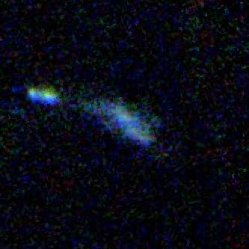
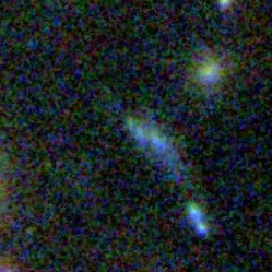
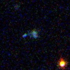
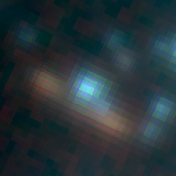
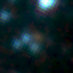
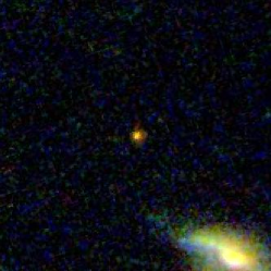
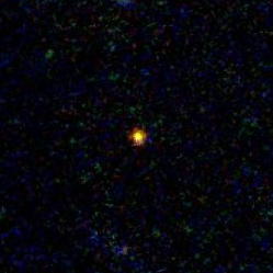
Figure 1.— Color composites of the three multiple image systems: F (top) and the two of K (middle) and L (bottom). $Viz$ color composite is used for systems F and L. System K is not detected in any of the optical bands; instead, we show Spitzer/IRAC $3.6\mu\mbox{m}$-$4.5\mu\mbox{m}$-$8\mu\mbox{m}$ images (see also Gonzalez et al. (2009). North is up and East is left in each panel. The cutouts are $10\arcsec\times 10\arcsec$.

The reconstruction is set up on an initial grid of $15\times 15$ pixels for a field of $9\arcmin\times 9\arcmin$. We then adapt the grid as follows. We have the highest S/N ratio in areas close to the observed multiple images; in addition, the S/N ratio declines as we go towards the outskirts of the cluster. We therefore refine the circular regions of $1\arcmin$ diameter around the centers of the main and the subcluster by a factor of 8 (i.e. each grid is split into $8\times 8$ grid points), by a factor of 4 in an annuli between $1\arcmin$ and $1.5\arcmin$, and by a factor of 2 in an annuli between $1.5\arcmin$ and $2\arcmin$. We also refine cells surrounding $0.5\arcmin$ around each multiply imaged system by 16. The resulting grid structure is visible in Fig. 2: the smallest cells have sizes of $2.25\arcsec$, corresponding to $\sim 10\mbox{ kpc}$ and to the Einstein diameter of massive ellipticals.

Only for system A has a spectroscopic redshift been obtained (Mehlert et al. 2001). Hence, we first perform the initial reconstruction using redshifts given in Bradač et al. (2006), which are a combination of photometric redshifts and lensing predictions from a smooth, simply-parametrized model. Then, we project all the images for each source to the source plane, take the average source position and calculate the rms difference between the measured image positions and those predicted by the model for the average source. We then vary the source redshift (while keeping the mass reconstruction fixed) around its predicted value given in Bradač et al. (2006). The redshift with the smallest rms for each of the sources is given in Table 1. The final surface mass density maps is given in Figure 3, together with the X-ray brightness contours. The average rms in predicted image positions per image (and source) is $1.4\arcsec$. The reconstruction has improved significantly with respect to our earlier map (in Bradač et al. 2006 the average rms was $4\arcsec$). The rms residuals depend upon the final adopted grid size. Whereas the final grid size could be further decreased, we chose not to do so, as the lack of redshift information limits our ability to reconstruct these small scales. We can achieve similar fits by adding small scale substructure close to the images, or changing their redshifts. Hence, in order to improve the mass reconstruction even further, we will need spectroscopic redshifts for more than one system, which are not presently available.

The statistical uncertainties in the redshifts of the multiply imaged sources can be estimated while keeping the mass reconstruction fixed. However, these are small and do not represent the true uncertainties. We would need to simultaneously vary the lens model and the redshifts to obtain true errors; this, however, is extremely computationally intensive. At present, however we mimic redshift uncertainties by adding small scale mass perturbations to the model in Section 5. As the two are degenerate, the perturbations that produce the shifts in the predicted positions of the multiple images larger than the rms residuals quoted above will give us conservative errors on the model.

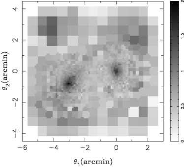
Figure 2.— The reconstructed surface mass density $\kappa$ of the cluster for a fiducial source at infinite redshift, $z_{\rm s}\to\infty$.

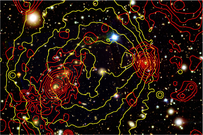
Figure 3.— The $Viz$ (main cluster) and F435W-$V$-F814W (sub cluster) color composite of the 1E0657$-$56 (catalog ). The ACS images are inset on the colour image from NASA Press release 06-297. Overlaid in red contours is the surface mass density $\kappa$ from the combined weak and strong lensing mass reconstruction. The contour levels are linearly spaced with $\Delta\kappa=0.1$, starting at $\kappa=0.7$, for a fiducial source at a redshift of $z_{\rm s}\to\infty$. The X-ray brightness contours from the 500 ks Chandra ACIS-I observations (Markevitch et al. 2006) are overlaid in yellow. North is up and East is left, the field is $7.4^{\prime}\times 5.3^{\prime}$, which corresponds to $2000\times 1400\mbox{ kpc}^{2}$ at the redshift of the cluster. The color composite was created following the algorithm from Lupton et al. (2004) and using the image from NASA Press release 06-297.

Table 1The properties of the multiply-imaged systems used in this work.

	Ra	Dec	$z_{\rm pred}(z_{\rm pred06})$
	104.65852	$-$55.950585
K	104.65447	$-$55.951904	2.8 (N/A)
	104.63917	$-$55.958060
	104.65024	$-$55.961577
L	104.64327	$-$55.963856	5.7 (N/A)
	104.64694	$-$55.958465
F	104.65209	$-$55.956241	0.9 (0.8)
	104.66497	$-$55.951324
	104.63316	-55.941395
A	104.62988	-55.943798	3.24 (3.24)
	104.62954	-55.941844
B	104.63042	-55.941474	3.9 (4.8)
	104.63775	-55.941851
C	104.63338	-55.945324	2.3 (2.1)
	104.64709	-55.943575
D	104.63528	-55.951836	1.5 (1.4)
	104.64008	-55.950620
E	104.64232	-55.948784	0.9 (1.0)
	104.56568	-55.939832
G	104.56402	-55.942113	1.1 (1.3)
	104.56417	-55.944131
	104.56293	-55.939764
H	104.56133	-55.942430	2.1 (1.9)
	104.56189	-55.947724
	104.56186	-55.946114
I	104.56052	-55.942930	2.3 (2.1)
	104.56141	-55.944264
	104.56909	-55.946016
J	104.57025	-55.944050	1.3 (1.7)

5. Bullet Cluster as a Cosmic Telescope: Lyman Break Galaxies at $z\sim 5-6$

In this section we present a search for $V$ and $i$-band dropout galaxies behind the Bullet Cluster.

5.1. Dropout selection and photometry

Galaxies were detected in the HST/ACS $Viz$ imaging data described in Section 3; we followed a procedure almost identical to that of Stark et al. (2009) and Coe et al. (2006). Faint objects were detected from a combined $Viz$ image, and colors measured in apertures of $0.6^{\arcsec}$ diameter. The foreground galactic extinction was corrected following Schlegel et al. (1998) and Cardelli et al. (1989). We also applied an aperture correction for the F850LP image of $-0.05$ following Coe et al. (2006). The total magnitudes in each band were computed using a combination of aperture color and SExtractor parameter MAG_AUTO from the reddest filter F850LP. We then selected filter dropouts with the same criteria as used in Stark et al. (2009) (and also in Beckwith et al. (2006)). For $V$-dropouts we require all of the following:

$$(V-i>1.47+0.89(i-z))\;\;{\rm or}\;\;(V-i>2)$$ (3)

$$V-i>1.2$$ (4)

$$i-z<1.3$$ (5)

$$S/N(z)>5$$ (6)

and since we do not have $B$-band data, we omit the last selection criterion from Stark et al. (2009). This does not significantly affect our results, as there are very few possible objects that would drop out in V and be detected in B (e.g. an AGN in a dusty galaxy). In addition, the study of Bouwens et al. (2007), which we also compare to, does not use B-band non-detection either. For $i$-dropouts we use:

$$i-z>1.3$$ (7)

$$S/N(z)>5$$ (8)

$$(S/N(V_{606})<2)\;\;{\rm or}\;\;(V-z>2.8) \>.$$ (9)

In addition, we rejected stars using the IMCAT software. We determined the significance and size of each object in each passband by convolving the images with a series of Mexican hat filters and determining the smoothing radius, $r_{\rm g}$, at which the filtered objects achieved maximum significance. This procedure, usually used for weak lensing analyses (see e.g. Clowe et al. 2006b), gives a better estimate of the size than SExtractor. We then identified stars from the $r_{\rm g}$ vs. magnitude diagram and rejected the bright stars ($m_{\rm z}<22$). Finally, we visually examined each object from the catalog in the images, removing any additional faint stars, artifacts (at the detector edges) from the sample. The visual inspection is successful in removing stars with ($m_{\rm z}<26$), at magnitudes 26-27, however, the fraction of stellar contaminants is negligible (Bouwens & Illingworth 2006). Our final sample comprises 20 $V$ and 4 $i$-band dropouts, their positions are given in Table 2 and the cutout images are shown in Figures 4 and 5.

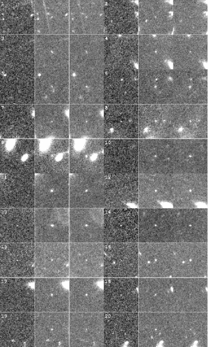
Figure 4.— Cutouts of $V$-band dropouts. The cutouts are shown for filters $Viz$ (in two columns), labels correspond to labels in Table 2. The sizes are $10\arcsec\times 10\arcsec$.

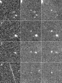
Figure 5.— Same as Fig. 4, except for $i$-band dropouts.

5.2. Estimate of the completeness and “lensed” number counts

To estimate the completeness of the sample we ran simulations using IRAF task artdata. We generated 1000 objects each at the average $z$-band magnitude $m_{\rm z}$ of $\{24,25,26,27,28\}$, with colors corresponding to a template spectrum from Bruzual A. & Charlot (1993) for a low metallicity ($Z=0.4\>Z_{\odot}$) starburst galaxy with an age of $125$ Myr and no dust. We assigned random redshifts to the galaxies (uniformly distributed in $4.0<z<5.9$ for $V$, and $5.0<z<7.6$ for $i$-band dropouts), and then follow Madau et al. (1996) in applying a corresponding IGM absorption correction. The galaxies were added to the $Viz$ images of the cluster and detected following the same procedure. The completeness levels are $>95\%$ for $m_{\rm z}=24$, 90% for $m_{\rm z}=25$, 50% for $m_{\rm z}=26$, and 5% at $m_{\rm z}=27$. To estimate the completeness for each individual object having $m_{\rm z}<27$, a fourth order polynomial as a function of $m_{\rm z}$ was fitted through above estimated completeness levels. The objects were then later added to the appropriate bins, assuming these completeness factors. We exclude any objects having (lensed, measured) magnitudes $m_{\rm z}\geq 27$ when calculating numbercounts of objects as a function of magnitude (see Fig. 6). The size of the field is $10.24\mbox{ arcmin}^{2}$.

We can now calculate the surface densities for our two dropout samples and compare them to values from the literature (we choose Stark et al. 2009, Bouwens et al. 2007, Beckwith et al. 2006 as they use the same filter-set and a comparison is straightforward). We bin our data in two bins of $m_{\rm z}=[25-26]$ and $[26-27]$ for $V$ and one bin $m_{\rm z}=[25-26.5]$ for $i$-dropouts. For the comparison with the literature the bins are then divided by 2 and 3 respectively to obtain counts in $0.5$-mag bins. Our results are presented as grey open circles with dashed errorbars in Fig. 6 (the determination of the “unlensed”, true number counts —shown as black solid circles in Fig. 6— will be described in Section 5.3). The errors include both Poisson errors and sample variance (also commonly referred to as cosmic variance). To calculate the sample variance we use the prescription from Somerville et al. (2004) and the correlation function from Nagamine et al. (2007). The sample variance for a single ACS field at $z\sim 6$ is $50\%$, which is also in agreement with sample variance calculator by Trenti & Stiavelli (2008). We immediately note that the lensing effect has increased the number of detected dropouts compared to blank surveys with similar or better exposure times to ours. Even though gravitational lensing effectively makes the actual observed solid angle smaller (due to magnification), the effective slope of the luminosity function $\Phi$ is steep at these magnitudes ($-\rm d(\log\Phi)/d(\log L)\gtrsim 1$), hence we increase the expected number density of sources by going deeper.

5.3. Number counts including magnification correction

To evaluate the true (unlensed) number counts, we use the mass reconstruction described in Section 4 to estimate the effective change in survey area. We use the deflection angle map for a redshift $z=5$ source for the $V$-dropouts, and for a $z=6$ source for the $i$-dropouts. We project the observed field from the lens plane to the source plane pixel by pixel and measure the corresponding change in solid angle by simple numerical integration. This resulted in a fractional area decrease of $0.25\pm 0.02$ for $z=5$ and $z=6$ case. The total shrinking of the field changes little with redshift, as the lensing strength (or angular diameter distance ratio between lens and source, and observer and source) at these redshifts for a lens at $z\sim 0.3$ is nearly constant (see e.g Bartelmann & Schneider 2001). The uncertainty was estimated by evaluating the area change using the magnification error map (described below). Neither a source redshift change (supported by the calculated solid angle change for sources at $z=5$ and 6) nor the magnification errors have a significant effect on the survey area shrinkage. The position of the critical curves changes by $\sim 5\mbox{ arcsec}$ between $z=5$ and $z\to\infty$, which is larger than the expected accuracy; even so, this has an almost negligible effect (within the errors quoted above) on the total solid angle change of the field.

Next we need to evaluate what the apparent magnitudes of the sources would have been in the absence of lensing. For this, we evaluate individual magnifications at the positions of these sources using our lens model. The errors on each magnification come from the errors on the mass reconstruction, and typically increase as the image approaches the critical curve. These errors are dominated by small-scale substructure not accounted for in the lens modeling, and by erroneous redshifts of multiple images used for the reconstruction. They are less affected by the typical uncertainties in cluster mass profile as discussed below.

5.4. Errors on magnification

To estimate the errors we used (for convenience) the approximate parametrized model for the Bullet Cluster (consisting of one PIEMD (pseudo-isothermal elliptical mass density, see e.g. Limousin et al. 2005) component for each of the main and subcluster, as well as 30 SIS (Singular Isothermal Spheres) placed over the full mass-reconstruction field representing the cluster galaxies (these are the confirmed cluster members in the inner $5\arcmin\times 3\arcmin$ field). These galaxies were taken to have line-of-sight velocity dispersion $\sigma_{\rm memb}$ following $\sigma_{\rm memb}\propto L^{1/4}$ and a fiducial galaxy with a F606W-band magnitude $m_{\rm F606W}=18$ has $\sigma_{\rm memb,18}=250{\rm\>km\>s}^{-1}$. We chose singular rather than non-singular isothermal spheres, as they will create larger local magnification changes. In addition, strong lensing studies of galaxy-scale lenses show that they have steep mass profiles in the centre, and hence small core radii (see e.g. Keeton 2003).

The above model gives us a manageable smooth model for the cluster mass distribution. To model the errors on the magnification due to substructure, we also randomly distributed 50 mass clumps with position covering our $Viz$ images (where dropouts were searched for) and magnitudes between $m_{\rm F606W}=22\mbox{ - }24$ (and the same scaling of mass as used above). Again, we are trying to maximize the magnification perturbations, hence using singular profiles is conservative. The mass fraction in these substructures was $\sim 8\%$; this is purposely high, since we want to be conservative in estimating the magnification errors. This model does not reproduce the multiple image positions in detail (i.e. we did not search for the best-fit model - the substructure fraction would have been lower and systematic errors due to uncertainties in redshifts and the main lens profile would be underestimated); however this is not needed for the error estimation. This additional substructure changes the critical curve positions by $5-10\mbox{ arcsec}$, which is more than the uncertainty with which multiple images are recovered (in this and in other well-modeled clusters, see e.g. Jullo & Kneib 2009). We generated 100 realisations of cluster substructure in this way, and then evaluated the magnification error as the standard deviation of the mean magnification at each pixel. The map of standard deviation in the change of magnitude $\sigma_{\rm mag}\simeq\sigma_{\mu}/\left\langle\mu\right\rangle$ as a function of position is given in Fig. 7. On average the errors are small across the observable field, only in the vicinity of the critical curve the errors become large. The errors at the positions of the dropouts are given in Table 2.

In addition, the average error $\left\langle\sigma_{\rm mag}\right\rangle$ as a function of average magnification $\left\langle\mu\right\rangle$ is shown in Fig. 8. As a comparison we also give the cumulative area as a function of magnification $\mu$, this time calculated for our reconstructed magnification map from Section 3. These plots illustrate that less than $0.1\mbox{ arcmin}^{2}$ of the survey (i.e. $<1\%$ of the area for a single pointing ACS observation) has magnifications $\mu>10$ and on average low errors. It is true, that we are more likely to find images in regions of large magnification; however only 3 out of 20 systems have highly uncertain magnifications (see Table 2). Hence the errors on the positions of the magnitude bins in evaluating the number counts (Fig. 6) are much smaller than the bin widths.

Above investigations use a fixed smooth model to determine uncertainties. To further evaluate uncertainties due to profile uncertainties, we have investigated magnification properties of three very different smooth profiles, singular isothermal sphere (SIS), non-singular isothermal sphere (NIS) and Navarro Frenk and White (NFW) profile. NFW and NIS profiles give rise to two critical curves, radial and tangential, whereas SIS’s radial critical curve shrinks to zero size. The existence of radial arcs and simulations tell us that SIS is not a valid description for cluster mass distribution. Systems with $\geq 2$ multiply imaged systems with known redshifts (like the one used here), and even more so, with included weak lensing information can distinguish between these profiles (see e.g. Sand et al. 2008, Limousin et al. 2008).

Still, we have investigated their magnification properties. First we match the Einstein radii of all three models, which is easily measured in practice even with a single multiply imaged system with known redshift. If also matching the radial critical curve, the change in area (due to magnification) is $<1\%$. If only the tangential critical curve is matched, and the radial ones differ by $\sim 10\mbox{ arcsec}$ these changes are still below $<20\%$, only when we compare SIS with NFW is the change in area significant. It is only significant for small observing fields (like the one used here) and can be as high as $50\%$, however this case is unrealistic as noted before. Furthermore, for a field twice this size, the errors due to uncertainties in smooth model are again below $5\%$. The individual magnifications differ by $<20\%$ everywhere outside the tangential critical curve and are mostly in $5\%$ regime, which is where most of our sources are located.

In conclusion, the errors due to lensing are smaller than the sample variance. Taking into account sub-dominant errors, the increased number of objects detected, and the ability to reach otherwise unobservably faint magnitudes, it is advantageous to use well-modeled clusters as cosmic telescopes to measure the average properties of background ($z\gtrsim 5$) objects, including their luminosity function. This conclusion is not limited only to high-redshift sources. The system K is at $z\sim 2.7$, but magnification factors of $\mu\sim 50$ make this ordinary (i.e. not ultra-luminous) sub-mm source detectable with Spitzer/IRAC (Gonzalez et al. 2009), AzTEC (Atacama Submillimeter Telescope Experiment, Wilson et al. 2008 and BLAST (Balloon-borne Large-Aperture Submillimeter Telescope, Rex et al. 2009).

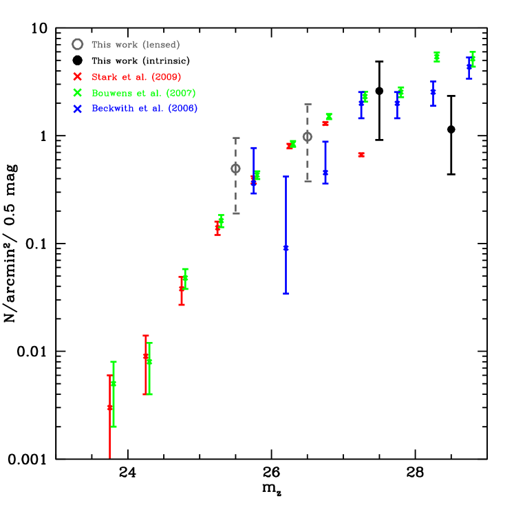
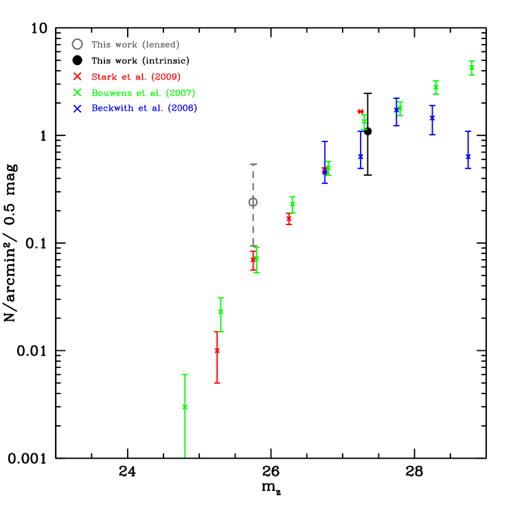
Figure 6.— Surface densities (number per $\mbox{arcmin}^{2}$ per $0.5\mbox{ mag}$) of $V$ (left) and $i$-band (right) dropouts (circles). Due to small number statistics, we bin the data in two bins of $m_{\rm z}=[25-26]$ and $[26-27]$ for $V$ and one bin $m_{\rm z}=[25-26.5]$ for $i$-dropouts and recalculate them to $0.5$-mag bins, which is the binning used in the literature (crosses). Only sources for which our completeness is greater than 5% (i.e. those with $m_{\rm z}<27$) are presented and completeness corrections are discussed in the text. Direct measurements (gray open circles with dashed errorbars) have been corrected for the effect of gravitational lensing, giving the intrinsic (unlensed) number counts (black full circles with solid errorbars). The errors for our data include sample variance, Poisson errors, and errors due to lensing (the latter of which are small in comparison). The crosses are all calculated for the bins indicated by Stark et al. (2009) data, the other two are shifted by 0.05 and 0.1 mag for clarity. Bouwens et al. (2007), and Stark et al. (2009) data have been corrected for completeness, whereas Beckwith et al. (2006) data were not. The Stark et al. (2009) points were calculated using GOODS data, Beckwith et al. (2006) only include HUDF number counts, whereas Bouwens et al. (2007) use data from HUDF, HUDF-Ps, and GOODS.

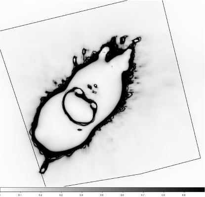
Figure 7.— The error on intrinsic (unlensed) source magnitude $\sigma_{\rm mag}$ (grey-shade) as a function of position. Most of the lens-plane area has errors $<0.1\mbox{ mag}$. The field we study here is approximately centered on the main cluster and is given as a box. The map assumes a source at $z\to\infty$, the map for $z=5$ or 6 would differ very little from the one presented here.

Figure 8.— Top: the average error on magnitude $\left\langle\sigma_{\rm mag}\right\rangle$ as a function of magnification. For magnifications of $\mu<10$, the errors are $<0.1\mbox{ mag}$ on average. The exact error as a function of location is given in Fig. 7. Bottom: cumulative number of image plane pixels having magnifications larger than a certain value. $<1\%$ of the pixels will have $\mu>10$, which is the only regime where the errors are of any significance for determining the intrinsic luminosity of a sample. Both plots assume a source at $z\to\infty$.

Table 2The properties of $V$-dropouts (top) and $i$-dropouts (bottom).

	Ra	Dec	$m_{\rm z}\pm\Delta_{\rm phot}$	$(V-i)$	$(i-z)$	$\mu$	$m_{\rm z,int}\pm\Delta_{\rm l+p}$
1	$104.59377$	$-55.970039$	$26.74\pm 0.07$	$2.2\pm 0.4$	$0.69\pm 0.14$	$2.68\pm 0.08$	$27.81^{+0.08}_{-0.08}$
2	$104.60201$	$-55.954700$	$27.89\pm 0.10$	$1.8\pm 0.2$	$-2.42\pm 0.15$	$3.97\pm 0.26$	$29.39^{+0.12}_{-0.12}$
3	$104.60582$	$-55.969944$	$26.45\pm 0.06$	$>1.5$	$0.20\pm 0.11$	$3.17\pm 0.09$	$27.70^{+0.07}_{-0.07}$
4	$104.61459$	$-55.951771$	$27.42\pm 0.05$	$2.2\pm 0.1$	$-0.54\pm 0.10$	$4.0\pm 0.9$	$28.93^{+0.23}_{-0.28}$
5	$104.61855$	$-55.940559$	$26.24\pm 0.05$	$3.3\pm 0.5$	$0.86\pm 0.13$	$5.8\pm 1.2$	$28.15^{+0.21}_{-0.26}$
6	$104.63613$	$-55.925079$	$25.53\pm 0.05$	$2.3\pm 0.6$	$0.59\pm 0.10$	$3.78\pm 0.15$	$26.98^{+0.07}_{-0.07}$
7	$104.64101$	$-55.935631$	$26.97\pm 0.05$	$2.3\pm 0.7$	$1.17\pm 0.13$	$6^{+15}_{-5}$	$29^{+2}_{-2}$
8	$104.64129$	$-55.964703$	$26.38\pm 0.06$	$2.3\pm 0.2$	$0.14\pm 0.11$	$12\pm 2$	$29.09^{+0.18}_{-0.21}$
9	$104.64133$	$-55.966335$	$25.04\pm 0.05$	$2.5\pm 0.4$	$0.97\pm 0.11$	$10\pm 1$	$27.54^{+0.11}_{-0.12}$
10	$104.64437$	$-55.973896$	$25.81\pm 0.05$	$2.4\pm 0.6$	$0.87\pm 0.10$	$5.2\pm 0.3$	$27.64^{+0.08}_{-0.08}$
11	$104.64603$	$-55.969257$	$25.68\pm 0.05$	$2.8\pm 0.3$	$-0.11\pm 0.10$	$6.5\pm 0.8$	$27.70^{+0.14}_{-0.15}$
12	$104.65024$	$-55.961578$	$25.52\pm 0.05$	$5.7\pm 4.0$	$0.88\pm 0.10$	$480\pm 30$	$32.22^{+0.08}_{-0.09}$
13	$104.65026$	$-55.966267$	$25.53\pm 0.05$	$2.6\pm 0.2$	$0.18\pm 0.10$	$30_{-29}^{+1000}$	$29^{+4}_{-4}$
14	$104.65306$	$-55.930065$	$26.30\pm 0.05$	$2.1\pm 0.1$	$0.12\pm 0.10$	$4.6\pm 0.2$	$27.96^{+0.07}_{-0.07}$
15	$104.65884$	$-55.948055$	$27.23\pm 0.06$	$4.0\pm 0.2$	$0.06\pm 0.11$	$207\pm 3$	$33.02^{+0.06}_{-0.06}$
16	$104.66796$	$-55.949810$	$25.60\pm 0.05$	$3.2\pm 0.6$	$0.72\pm 0.10$	$34^{+100}_{-33}$	$29^{+2}_{-4}$
17	$104.67584$	$-55.945240$	$26.01\pm 0.05$	$3\pm 1.0$	$0.32\pm 0.10$	$7\pm 1.0$	$28.19^{+0.15}_{-0.17}$
18	$104.67677$	$-55.943958$	$28.18\pm 0.05$	$1.5\pm 0.10$	$-1.42\pm 0.10$	$7.1\pm 0.5$	$30.31^{+0.09}_{-0.09}$
19	$104.68509$	$-55.951725$	$27.14\pm 0.05$	$3.9\pm 0.2$	$-0.23\pm 0.10$	$8.6\pm 0.4$	$29.47^{+0.07}_{-0.07}$
20	$104.68786$	$-55.943943$	$27.36\pm 0.09$	$2.2\pm 0.5$	$-0.05\pm 0.14$	$4.8\pm 0.2$	$29.06^{+0.10}_{-0.10}$
1	$104.63920$	$-55.925922$	$26.29\pm 0.05$	$>0.5$	$1.33\pm 0.10$	$4.9\pm 0.2$	$28.01_{-0.07}^{+0.07}$
2	$104.65271$	$-55.930984$	$25.44\pm 0.05$	$>1.4$	$1.33\pm 0.10$	$4.6\pm 0.2$	$27.10_{-0.07}^{+0.07}$
3	$104.66599$	$-55.931286$	$25.38\pm 0.05$	$2\pm 1$	$1.34\pm 0.11$	$3.4\pm 0.2$	$26.71_{-0.08}^{+0.08}$
4	$104.67469$	$-55.929668$	$26.04\pm 0.05$	$>0.5$	$1.71\pm 0.13$	$3.1\pm 0.1$	$27.26_{-0.06}^{+0.06}$

Note. — For the final error on $m_{\rm z,int}$ ($\Delta_{\rm l+p}$) photometric and magnification errors were added in quadrature.

6. Conclusions and Outlook

We have presented a new mass reconstruction for the post-collision Bullet Cluster. In addition, we have used its extraordinary capabilities as a cosmic telescope to study $z\sim 5-6$ objects. Our main conclusions are as follows:

1. Our new strong and weak lensing mass reconstruction method, that uses a non-uniform adaptive pixel grid, performs very well in reconstructing the cluster potential in the vicinity of multiple images. In particular, we have improved the accuracy with which the image positions are reproduced to an average rms residual of $1.4\arcsec$. The limitation in pushing this number to the observed uncertainties in image position ($\sim 0.1\arcsec$) is mostly in the lack of secure redshifts (only one spectroscopic redshift is known for the 12 multiple image systems used here). The method can resolve the small scale substructure and reconstruct the images even more precisely, once the redshifts become available.

2. Bullet Cluster is an efficient cosmic telescope. We have used its power to search for $z\sim 5-6$ objects using the dropout technique. After correcting for the lensing effect and taking into account the errors from the imperfect magnification map, we derive the surface densities of $V$ and $i$-band dropouts. They match well the densities (in absolute value) derived from previous studies (Stark et al. 2009, Bouwens et al. 2007, Beckwith et al. 2006) using either deeper or larger surveys (HUDF and GOODS). E.g. GOODS (release 1) data has similar exposure times ($5000\mbox{s}$ in $V$ and $i$ and $10660$ in $z$) over $360\mbox{ arcmin}^{2}$ field. Scaling total numbers of dropouts from Stark et al. (2009) (using area ratio between our and their survey) we would obtain 14 $V$ and 3.5 $i$-band dropouts; whereas we observe 20 and 4. In addition they are at fainter (intrinsic) magnitudes as their sample.

3. Our sample numbers are much smaller (as our search area is $10\mbox{ arcmin}^{2}$, compared to the area used in e.g. Stark et al. (2009), Bouwens et al. (2007) with $>300\mbox{ arcmin}^{2}$), and so the errorbars are dominated by sample variance and Poisson noise. However, our results show, that at the same observed magnitudes, we gain in the number of sources observed compared to a blank field of the same size. In addition, we observe intrinsically fainter sources than would otherwise be possible in a blank field observed to similar depths. Finally, multiply imaged sources are easily discriminated from contaminants, as lens model roughly predicts their redshifts, and hence can be distinguished from $z\sim 2$ dusty galaxy and cool stars.

This analysis can and will be extended to higher redshift objects (z and J-dropouts). The main requirement for such studies is deep optical and near-IR data, as well as high resolution magnification maps such as the one presented in this paper. These studies can also be readily expanded to a larger sample of clusters. With a sample of $\sim 20$ massive clusters, with well understood magnification properties and observed to similar depths as the Bullet Cluster we can increase the expected number counts and reduce the errors due to sample variance and Poisson sampling to those of GOODS (see e.g. Stark et al. 2009). However, due to lensing, we can push observations to at least a magnitude deeper than GOODS and only slightly shallower than HUDF (in much shorter observing time). Finally, highly magnified images ($\mu\gtrsim 50$) potentially allow for (otherwise prohibitive) spectroscopic follow up of these high redshift galaxies. Highly magnified objects will often sample populations that would otherwise be unobservable by any practical means.

References

- Abramowitz & Stegun (1972) Abramowitz, M., & Stegun, I. A. 1972, Handbook of Mathematical Functions (Handbook of Mathematical Functions, New York: Dover, 1972)
- Bacon et al. (2006) Bacon, D. J., Goldberg, D. M., Rowe, B. T. P., & Taylor, A. N. 2006, MNRAS, 365, 414
- Barrena et al. (2002) Barrena, R., Biviano, A., Ramella, M., Falco, E. E., & Seitz, S. 2002, A&A, 386, 816
- Bartelmann et al. (1996) Bartelmann, M., Narayan, R., Seitz, S., & Schneider, P. 1996, ApJ, 464, L115
- Bartelmann & Schneider (2001) Bartelmann, M., & Schneider, P. 2001, Phys. Rep., 340, 291
- Beckwith et al. (2006) Beckwith, S. V. W., et al. 2006, AJ, 132, 1729
- Bertin & Arnouts (1996) Bertin, E., & Arnouts, S. 1996, A&AS, 117, 393
- Bouwens & Illingworth (2006) Bouwens, R. J., & Illingworth, G. D. 2006, Nature, 443, 189
- Bouwens et al. (2009a) Bouwens, R. J., et al. 2009a, ApJ, 690, 1764
- Bouwens et al. (2007) Bouwens, R. J., Illingworth, G. D., Franx, M., & Ford, H. 2007, ApJ, 670, 928
- Bouwens et al. (2008) Bouwens, R. J., Illingworth, G. D., Franx, M., & Ford, H. 2008, ApJ, 686, 230
- Bouwens et al. (2009b) Bouwens, R. J., et al. 2009b, ArXiv:0909.1803
- Bouwens et al. (2005) Bouwens, R. J., Illingworth, G. D., Thompson, R. I., & Franx, M. 2005, ApJ, 624, L5
- Bradač et al. (2008a) Bradač, M., Allen, S. W., Treu, T., Ebeling, H., Massey, R., Morris, R. G., von der Linden, A., & Applegate, D. 2008a, ApJ, 687, 959
- Bradač et al. (2006) Bradač, M., et al. 2006, ApJ, 652, 937
- Bradač et al. (2005) Bradač, M., Schneider, P., Lombardi, M., & Erben, T. 2005, A&A, 437, 39
- Bradač et al. (2008b) Bradač, M., et al. 2008b, ApJ, 681, 187
- Bradley et al. (2008) Bradley, L. D., et al. 2008, ApJ, 678, 647
- Bruzual A. & Charlot (1993) Bruzual A., G., & Charlot, S. 1993, ApJ, 405, 538
- Bunker et al. (2009) Bunker, A., et al. 2009, ArXiv:0909.2255
- Cardelli et al. (1989) Cardelli, J. A., Clayton, G. C., & Mathis, J. S. 1989, ApJ, 345, 245
- Clowe et al. (2006a) Clowe, D., Bradač, M., Gonzalez, A. H., Markevitch, M., Randall, S. W., Jones, C., & Zaritsky, D. 2006a, ApJ, 648, L109
- Clowe et al. (2006b) Clowe, D., et al. 2006b, A&A, 451, 395
- Coe et al. (2006) Coe, D., Benítez, N., Sánchez, S. F., Jee, M., Bouwens, R., & Ford, H. 2006, AJ, 132, 926
- Deb et al. (2008) Deb, S., Goldberg, D. M., & Ramdass, V. J. 2008, ApJ, 687, 39
- Diego et al. (2007) Diego, J. M., Tegmark, M., Protopapas, P., & Sandvik, H. B. 2007, MNRAS, 375, 958
- Ellis et al. (2001) Ellis, R., Santos, M. R., Kneib, J., & Kuijken, K. 2001, ApJ, 560, L119
- Giavalisco (2002) Giavalisco, M. 2002, ARA&A, 40, 579
- Giavalisco et al. (2004a) Giavalisco, M., et al. 2004a, ApJ, 600, L103
- Giavalisco et al. (2004b) Giavalisco, M., et al. 2004b, ApJ, 600, L93
- Gonzalez et al. (2009) Gonzalez, A. H., Clowe, D., Bradač, M., Zaritsky, D., Jones, C., & Markevitch, M. 2009, ApJ, 691, 525
- Henry et al. (2008) Henry, A. L., Malkan, M. A., Colbert, J. W., Siana, B., Teplitz, H. I., & McCarthy, P. 2008, ApJ, 680, L97
- Henry et al. (2009) Henry, A. L., et al. 2009, ApJ, 697, 1128
- Hildebrandt et al. (2009) Hildebrandt, H., Pielorz, J., Erben, T., van Waerbeke, L., Simon, P., & Capak, P. 2009, A&A, 498, 725
- Jullo & Kneib (2009) Jullo, E., & Kneib, J.-P. 2009, MNRAS, 395, 1319
- Keeton (2003) Keeton, C. R. 2003, ApJ, 582, 17
- Kneib et al. (2004) Kneib, J., Ellis, R. S., Santos, M. R., & Richard, J. 2004, ApJ, 607, 697
- Koekemoer et al. (2002) Koekemoer, A. M., Fruchter, A. S., Hook, R. N., & Hack, W. 2002, in The 2002 HST Calibration Workshop, Baltimore, MD, 2002., p.339, 339
- Limousin et al. (2005) Limousin, M., Kneib, J.-P., & Natarajan, P. 2005, MNRAS, 356, 309
- Limousin et al. (2008) Limousin, M., et al. 2008, A&A, 489, 23
- Lupton et al. (2004) Lupton, R., Blanton, M. R., Fekete, G., Hogg, D. W., O’Mullane, W., Szalay, A., & Wherry, N. 2004, PASP, 116, 133
- Madau et al. (1996) Madau, P., Ferguson, H. C., Dickinson, M. E., Giavalisco, M., Steidel, C. C., & Fruchter, A. 1996, MNRAS, 283, 1388
- Markevitch et al. (2002) Markevitch, M., Gonzalez, A. H., David, L., Vikhlinin, A., Murray, S., Forman, W., Jones, C., & Tucker, W. 2002, ApJ, 567, L27
- Markevitch et al. (2006) Markevitch, M., Randall, S., Clowe, D., Gonzalez, A., & Bradac, M. 2006, in COSPAR, Plenary Meeting, Vol. 36, 36th COSPAR Scientific Assembly, 2655
- Marshall (2006) Marshall, P. 2006, MNRAS, 372, 1289
- McLure et al. (2009) McLure, R. J., Dunlop, J. S., Cirasuolo, M., Koekemoer, A. M., Sabbi, E., Stark, D. P., Targett, T. A., & Ellis, R. S. 2009, ArXiv:0909.2437
- Mehlert et al. (2001) Mehlert, D., Seitz, S., Saglia, R. P., Appenzeller, I., Bender, R., Fricke, K. J., Hoffmann, T. L., et al. 2001, A&A, 379, 96
- Merten et al. (2008) Merten, J., Cacciato, M., Meneghetti, M., Mignone, C., & Bartelmann, M. 2008, ArXiv:0806.1967
- Nagamine et al. (2007) Nagamine, K., Wolfe, A. M., Hernquist, L., & Springel, V. 2007, ApJ, 660, 945
- Oesch et al. (2009a) Oesch, P. A., et al. 2009a, ArXiv:0909.1806
- Oesch et al. (2009b) Oesch, P. A., et al. 2009b, ApJ, 690, 1350
- Reddy & Steidel (2009) Reddy, N. A., & Steidel, C. C. 2009, ApJ, 692, 778
- Rex et al. (2009) Rex, M., et al. 2009, ArXiv:0904.1203
- Richard et al. (2006) Richard, J., Pelló, R., Schaerer, D., Le Borgne, J.-F., & Kneib, J.-P. 2006, A&A, 456, 861
- Sand et al. (2008) Sand, D. J., Treu, T., Ellis, R. S., Smith, G. P., & Kneib, J.-P. 2008, ApJ, 674, 711
- Schlegel et al. (1998) Schlegel, D. J., Finkbeiner, D. P., & Davis, M. 1998, ApJ, 500, 525
- Schneider & Er (2008) Schneider, P., & Er, X. 2008, A&A, 485, 363
- Somerville et al. (2004) Somerville, R. S., Lee, K., Ferguson, H. C., Gardner, J. P., Moustakas, L. A., & Giavalisco, M. 2004, ApJ, 600, L171
- Soucail (1990) Soucail, G. 1990, Ap&SS, 170, 283
- Stanway et al. (2003) Stanway, E. R., Bunker, A. J., & McMahon, R. G. 2003, MNRAS, 342, 439
- Stanway et al. (2005) Stanway, E. R., McMahon, R. G., & Bunker, A. J. 2005, MNRAS, 359, 1184
- Stark et al. (2009) Stark, D. P., Ellis, R. S., Bunker, A., Bundy, K., Targett, T., Benson, A., & Lacy, M. 2009, ArXiv:0902.2907
- Steidel et al. (1996) Steidel, C. C., Giavalisco, M., Pettini, M., Dickinson, M., & Adelberger, K. L. 1996, ApJ, 462, L17
- Trenti & Stiavelli (2008) Trenti, M., & Stiavelli, M. 2008, ApJ, 676, 767
- Tucker et al. (1995) Tucker, W. H., Tananbaum, H., & Remillard, R. A. 1995, ApJ, 444, 532
- van den Bosch et al. (2003) van den Bosch, F. C., Yang, X., & Mo, H. J. 2003, MNRAS, 340, 771
- Vanzella et al. (2009) Vanzella, E., et al. 2009, ApJ, 695, 1163
- Wilson et al. (2008) Wilson, G. W., et al. 2008, MNRAS, 390, 1061
- Yan et al. (2009) Yan, H., Windhorst, R., Hathi, N., Cohen, S., Ryan, R., O’Connell, R., & McCarthy, P. 2009, ArXiv:0910.0077
- Yoshida et al. (2006) Yoshida, M., et al. 2006, ApJ, 653, 988
- Zheng et al. (2009) Zheng, W., et al. 2009, ApJ, 697, 1907