Implied Multi-Factor Model for Bespoke CDO Tranches
and other Portfolio Credit Derivatives
Igor Halperin
Quantitative Research, JP Morgan
Email: igor.halperin@jpmorgan.com
October 2009

Abstract:

This paper introduces a new semi-parametric approach to the pricing and risk management of bespoke CDO tranches, with a particular attention to bespokes that need to be mapped onto more than one reference portfolio. The only user input in our framework is a multi-factor model (a ”prior” model hereafter) for index portfolios, such as CDX.NA.IG or iTraxx Europe, that are chosen as benchmark securities for the pricing of a given bespoke CDO. Parameters of the prior model are fixed, and not tuned to match prices of benchmark index tranches. Instead, our calibration procedure amounts to a proper reweightening of the prior measure using the Minimum Cross Entropy method. As the latter problem reduces to convex optimization in a low dimensional space, our model is computationally efficient. Both the static (one-period) and dynamic versions of the model are presented. The latter can be used for pricing and risk management of more exotic instruments referencing bespoke portfolios, such as forward-starting tranches or tranche options, and for calculation of credit valuation adjustment (CVA) for bespoke tranches.

1 Introduction

It is well known that virtually all models for pricing and risk management of derivative securities are interpolators of different degrees of sophistication. Given observed market prices of various derivatives, the problem of pricing a new, illiquid security, whose price is not available from the marketplace, amounts to first finding benchmark traded (liquid) derivatives most similar to the one at hand, and then providing a rule by which their prices should be interpolated (and possibly extrapolated) in order to price our security.

The second step is where one needs a model. Complexity of the model depends on the instrument one needs to price, and on the market. In some cases, the model can be as simple as a one-dimensional spline (or even linear) interpolation. This is the case when e.g. an equity option with a given strike and maturity is priced by interpolating implied volatilities of benchmark traded options on the same underlying and with the same maturity. Note that generally such interpolation is done not directly in the price space, but in some ”model parameter space”, a procedure that should properly handle constraints imposed by the no-arbitrage principle, and also account for stochasticity of underlying price processes. In particular, as long as the underlying for both the illiquid and liquid options is the same, pricing by interpolation is relatively straightforward once one specifies a stochastic model for the underlying, calibrates it, and identifies relevant parameters that differentiate between the benchmark and the target derivatives.

In the case of correlation-dependent portfolio credit derivatives, the role of benchmark securities is played by standardized tranches referencing standard portfolios, called credit index portfolios, such as CDX.NA.IG or iTraxx Europe. Both these portfolios consist of synthetic exposures (in the credit default swap format) to 125 liquidly traded investment grade corporate obligors (“names”), added with equal weights. Index tranches are swap contracts covering portfolio losses between an attachment and detachment points (commonly referred to as strikes) that are expressed as a percentage of the total portfolio notional. Standardized strikes are 0, 3, 7, 10, 15, 30, 100 % for CDX.NA.IG index, and 0, 3, 6, 9, 12, 22, 100 % for iTraxx Europe index, and standard tradeable maturities are 5, 7, 10 and (to a lesser extend) 3 years. Other standard portfolios are somewhat less liquid, but still are more or less actively traded in the market. In particular, CDX.NA.HY index has 100 US non-investment grade (“high yield”) names, with standardized strikes of 0, 10, 15, 25, 35 and 100 %.

Market participants use quoted prices of standardized index tranches in order to estimate prices of other correlation-dependent derivatives, such as cash CDO tranches, non-standard tranches referencing standard index portfolios with strikes or/and maturities different from those actively traded, or customized (bespoke) synthetic tranches whose reference portfolios differ in their composition from credit index portfolios. More specifically, as prices of these instruments are driven by both observable (CDS prices) and unobservable parameters (in particular, parameters determining default dependencies under the risk-neutral measure, such as asset correlations in the Gaussian copula model), practitioners typically use market prices to estimate the latter set of parameters using a specific model, and then use (and possibly interpolate/extrapolate) these parameters within the same model to price the instrument in question.

In this paper, we address the problem of pricing sythnetic bespoke CDO tranches by unraveling of information contained in the market prices of benchmark index tranches. In the Street jargon, this is often referred to as “bespoke mapping problem”, implying that a given bespoke tranche is “mapped” onto index tranches. Obviously, this problem can be viewed as another example of pricing by interpolation. On the other hand, it is clear that, as long as composition of a bespoke portfolio is different from that of an index portfolio, the bespoke mapping problem is considerably more complicated than the above problem of pricing an illiquid equity option by interpolation of Black-Scholes implied volatilities. The reason is that the present case requires not only interpolation across strikes and/or maturities, but should also somehow involve interpolation/extrapolation across the underlying.

As the Gaussian copula with base correlations (and a possible extension to random recovery) continues, in spite of its well known drawbacks, to serve as the current market standard, practitioners usually pose the bespoke mapping problem as the base correlation mapping problem. The idea here is to find proper correlation parameters for a bespoke tranche at hand by a suitable adjustment of market-implied base correlations for standard index tranches, with an adjustment designed to account for differences between the index and bespoke portfolios.

While various base correlation mapping rules are used by practitioners, these rules are ad hoc and lack a theoretical or empirical justification. Worse yet, the base correlation method is theoretically inconsistent, and occasionally violates no-arbitrate constraints in practice, even when applied to a simpler problem of pricing non-standard tranches referencing the same index portfolio. Furthermore, being a one-factor model, the base correlation approach does not properly addresses the sector concentration risk, and thus cannot be expected to provide thustworthy results as long as composition of a bespoke portfolio is materially different from that of the reference index portfolio. More details on the base correlation mapping rules and their drawbacks will be given below.

In this paper we develop a consistent and practically oriented model for pricing despoke CDOs and other portfolio credit derivatives. We specifically concentrate on the case of bespokes that have to be mapped onto more than one reference index, which is often the case in practical settings, where a given bespoke portfolio can include e.g. both US and European names, or both investment and non-investment grade (IG and HY, respectively) names. Comparing to bespokes that need only be mapped onto one reference index, the latter case is more complex and produces higher modeling uncertainty. At the same time, it is also more computationally demanding, as it calls for a multi-factor framework (see below) in which one has to simultaneously calibrate to tranches written on all reference indices.

Our framework combines several modeling concepts, and generally belongs in the class of “implied distribution” models that have gained in popularity in recent years. We start with a bottom-up view of an index portfolio within a factor framework with a multivariate “market factor” $\vec{Z}$, where individual defaults are independent conditional on the value of $\vec{Z}$. Any arbitrage-free factor model of conditional independence type can be used here, examples are discussed below. This model is referred to as the prior model. At the next step, we departure from the usual bottom-up framework in two aspects. First, we assume that parameters in our prior model are fixed once and for all, i.e. we do not fit this model to available data. Second, we give up the fine resolution of the portfolio loss into contributions of individual obligors, and instead bucket all names in the index portfolio (and their respective losses) into two groups of names (sub-portfolios) according to their membership degree in the bespoke portfolio. In this way we construct a dichotomic representation of index portfolio losses as a joint loss distribution of two sub-portfolios. As an avatar of the factor framework we have started with, losses in the sub-portfolios are independent conditional on the market factor. This representation serves as a single object of further analysis.

In the second step, we calibrate our model by finding a minimal functional distortion of the prior dichotomic loss distributions of index portfolios needed in order to match observed prices of tranches referencing these portfolios. This is done within a semi-parametric framework based on the Minimum Cross Entropy (MCE) method, where the number of free parameters is data-driven, and is equal to the number of tradable tranches. The resulting joint loss distribution is then used to price tranches on a bespoke portfolio. Details of this procedure will be introduced in Sect.3.

The justification for taking a top-down view of the portfolio loss process is three-fold. First, market incompleteness imposes severe restrictions on the extent to which the ”true” (market-implied) risk-neutral measure can be learned. For example, for a standard portfolio like CDX.NA.IG or iTraxx Europe, the only available source of information about risk-neutral dependencies are tranche prices (6 quotes per maturity), which is not sufficient to infer the pricing measure in a unique way. The only way out is to model it using a low dimensional space of adjustable parameters. With our MCE approach, such a parametrization is constructed directly in the loss space, no-arbitrage relations are satisfied by construction, and calibration amounts to convex optimization. Second, as will be discussed in more details in Sect 2.4, the knowledge of dichotomic loss distributions of index portfolios is sufficient to price tranches on bespoke portfolios made of arbitrary compositions of ”chunks” of index portfolios, and can be readily generalized to other types of bespoke portfolios which involve names not belonging to any index. Third, our approach is computationally more efficient than a bottom-up one which can become quite computationally intense in a typical setting of pricing bespoke tranches that need be mapped onto more than one index portfolio.

The rest of this paper is organized as follows. The reminder of this introduction discusses base correlation mapping methods and explains the relation of our approach to the previous literature. In Sect.2 we provide a high-level qualitative overview of key elements of our modeling framework. Sect.3 provides technical details of the Minimum Cross Entropy (MCE) calibration scheme. Information-theoretic aspects of our problem are discussed in the appendix. In Sect.4 we present a dynamic version of the model. Sect.5 deals with generalization and extensions. Numerical examples are considered in Sect.6. The final Sect.7 concludes.

1.1 Base correlation mapping methods

A one-factor Gaussian copula model developed by Li [18] continues to be the market standard model. As in its original form the model is uncapable of matching market prices, practitioners use it in a way similar to the way the Black-Scholes model is used in other markets. Namely, traders convert market prices of index tranches into what is called base correlations. The latter are defined in two steps. First, one converts market prices into prices of synthetic equity tranches (base tranches) covering losses from 0 % to $K\%$, where $K$ is one of the standard strikes for the index under consideration. Second, base correlation $\beta(K)$ for strike $K$ is found as the correlation parameter that should be used by the Gaussian copula model in order to match the price of base tranche with strike $K$. Market prices typically imply an increasing “correlation skew” function $\beta(K)$.

Within the Gaussian copula/base correlation framework, the problem of pricing bespoke tranches amounts to calculating base correlations for a bespoke portfolio from base correlations for an index portfolio. This is achieved by first calculating strike $K_{i}$ of the index portfolio that is “equivalent” (in a sense defined below) to strike $K_{b}$ of the bespoke tranche, and then using interpolation of base correlations for standard strikes in order to find $\beta(K_{i})$. Several methods are used by traders to define what is meant by such “equivalence”:

• Absolute strike rule (no mapping): Here to price a bespoke tranche with strike $K_{b}$, we use the base correlation for the same strike, i.e. our rule is $K_{i}=K_{b}$. Such a naive rule is seldom used as it stands, as the probabilities to reach the same strike for a bespoke and index portfolio can be very different if e.g. their average spreads are vastly different.

• ATM mapping rule: Here one assumes that the observed correlation skew $\beta(t,K,L,\ldots)$ (written here as a general function of calendar time $t$, strike $K$, expected portfolio loss $L$ and possible other variables) is a function of $t$ and a single dimensionless ratio (“moneyness”) $x\equiv K/L$:

  $$\beta(t,K,L,\ldots)=\beta\left(t,x=\frac{K}{L}\right)$$ (1)

  (Note that if the skew is a function of only $t,K$ and $L$, then the ansatz (1) follows simply on the dimensional grounds.)

  Given expected losses $L_{b}$ and $L_{i}$ of the bespoke and index portfolios, respectively, the two portfolio will have the same $\beta$, and hence the same risk, when they have the same value of $x$. This yields the following relation for the index strike $K_{i}$ that is ”equivalent” to a given strike $K_{b}$ of the bespoke portfolio:

  $$\frac{K_{i}}{L_{i}}=\frac{K_{b}}{L_{b}}$$ (2)

  It is interesting to note that ansatz (1) has some dynamic implications for the behavior of the correlation skew. Indeed, let us calculate its partial derivatives:

  $$\frac{\partial\beta}{\partial K} = \frac{1}{L}\frac{d\beta}{dx}$$ (3)

  $$\frac{\partial\beta}{\partial L} = -\frac{K}{L^{2}}\frac{d\beta}{dx}=-\frac{K}{L}\frac{\partial\beta}{\partial K}$$

  If the skew is upward sloping, then the second of Eqs.(3) implies that $\partial\beta/\partial L\leq 0$, i.e. the skew moves downward as the expected portfolio loss (and hence the par portfolio spread) increases.

  If we assume that the correlation skew $\beta(t,x)$ is a slowly changing function of its first argument, i.e. its changes are largely driven by changes of $x$, then the latter prediction can be tested using the actual data. In Fig. 1 we show the profile of the correlation skew of the CDX.NA.IG11 index portfolio for 04/15/09 and 05/15/09. One sees that while the index spread goes down, the skew moves down as well. We conclude that the ATM rule (2) is likely to be in conflict with empirical data.

  

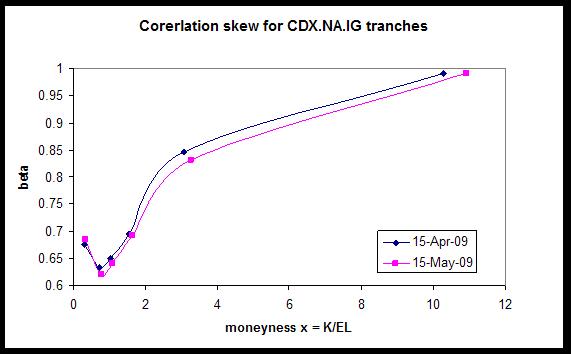
  Figure 1: Correlation skew for CDX.NA.IG11 as a function of moneyness. Expected portfolio loss is 9.72 % on 04/15/09 and 9.16 % on 05/15/09.

  What is missing in Eq.(2)? Note that the strike adjustment according to (2) is determined only by the portfolio expected loss and not e.g. higher moments of the loss distribution. This may appear counter-intuitive. Indeed, comparing two portfolios having e.g. the same average spread but different spread dispersion, we expect that the more dispersed portfolio should have higher risk under nearly any reasonable risk metric.

• Probability matching rule: $K_{i}$ is determined from the condition that cumulative probability of losses reaching strikes $K_{b}$ and $K_{i}$ for the bespoke and index portfolios should match:

  $$Pr\left(L_{i}\leq K_{i}\right)=Pr\left(L_{b}\leq K_{b}\right)$$ (4)

  This prescription takes higher moments of the loss distributions for the bespoke and index portfolio into account. However, the problem now is that the right-hand side (RHS) of (4) is only defined as long as the loss distribution for the bespoke is known, but the latter is exactly what we want to find in the first place! This means that on its own, Eq.(4) is incomplete, and thus potentially has an infinite number of solutions. The way the rule (4) is used in practice is to assume that its RHS can be computed using CreditMetrics/Base Correlation model with correlation $\beta(K_{i})$. When interpreted in this way, Eq.(4) becomes a highly non-linear equation for $K_{i}$, whose fixed point determines both the equivalent strike and the pricing measure for the bespoke. However, it is important to realize that this assumption is ad-hoc, and may lead to a sub-optimal and/or biased solution of the bespoke mapping problem. As a practical problem, the probability matching method does not always have a solution for bespokes with wide spreads.

While other similar recipes of base correlation mapping are available in the literature, see e.g. [24], the main problem with all these methods is that they are ad hoc and do not have a solid theoretical or empirical basis. In practice, their use leads at times to violation of no-arbitrage relations for bespoke portfolios across strikes or maturities.

Further problems with the use of base correlation mapping rules have to do with market incompleteness. Market prices of standard tranches provide only information on average risk-neutral default dependencies for a well-diversified (across different industrial sectors) index portfolio, and not information about default correlations specific to different industrial sectors. This implies that the base correlation method within a one-factor Gaussian copula framework does not capture sector concentration risk, and thus can be potentially dangerous to use for bespoke portfolios whose sector or/and geographical composition is materially different from that of standard portfolios. For a further discussion of practical difficulties arising with the use of base correlation approach for pricing bespoke tranches, see e.g. [24], [15] and [20].

1.2 Relation to previous literature

Our model combines elements of both bottom-up and top-down approaches. Here we would like to give a brief account of literature most relevant to our approach.

In a typical bottom-up model, we start at the view of a credit portfolio as a collection of separate exposures (”single names”), whose default dependencies are then introduced via a factor copula in structural models, or via a multi-variate intensity process. Any consistent multi-factor bottom-up model, with parameters tuned to roughly match the observed data, can be used as the “prior” model in our approach. Examples inlcude, in particular, the Gaussian copula model of Li [18], a multi-factor version of the RFL model [1], or reduced-form models, see e.g. Duffie and Garleanu [7], or Chapovsky et al [5].

Once the prior model is chosen, we switch to a top-down paradigm, concentrating on the dichotomic representation of portfolio losses (see above), and abstracting from the initial single-name picture. The idea of modeling credit portfolios in a top-down manner is originally due to Giesecke and Goldberg [8], Sidenius, Peterbarg and Andersen [22], and Schönbucher [21]. Our approach resembles the BSLP model of Arnsdorf and Halperin [2] in the sense that transition from the initial (“prior”) distribution to a “true” (calibrated) one is achived via a set of multiplicative loss-dependent factors applied directly to the portfolio loss distribution, though a particular realisation of this idea in the present framework is different.

Effectively, our procedure amounts to constructing loss distributions for both the index and bespoke portfolio in a way implied by observed prices of standard tranches. Thus our method belongs in the class of implied loss distribution approaches which have become quite popular among practitioners in recent years. Examples of such approach include e.g. the implied copula model of Hull and White [15], [16], or the factor model of Inglis and Lipton [17]. Unlike these authors, we work in a multi-factor setting that starts with a usual factor model, and consistently apply information-theoretic methods in order to construct implied loss distribution, while e.g. Hull and White adopt smoothness criteria as the main tool in their method.

In employing a multi-factor framework and using information-theoretic (entropy-based) methods for calibration, our approach is akin to that taken by Rosen and Saunders [20]. They develop an entropy-based calibration method for a class of multi-factor bottom-up models, where adjustment to market prices amounts to calculation of implied market factor distribution. Unlike the latter authors, we use a top-down entropy calibration where we calibrate to losses in tranches and suitably chosen sub-portfolios (see below), but not to individual names. This choice is made for the sake of simplicity and efficiency of implementation, and to facilitate an easy transition to a dynamic setting. On the implementation side, Rosen and Saunders employ a Monte Carlo scheme which is a preferred method when the number of market factors is three or more, while in our model we settle for a practically-oriented two-factor framework, and design an efficient lattice-based scheme for calibration and pricing, which is comparable in performance to the BSLP model of Ref.[2]. The main difference of our present framework from more traditional top-down approaches is that for pricing of bespoke tranches, we need a finer resolution of portfolio loss scanarios, which is achieved via calculation of joint loss distributions of sub-portfolios of credit indices. In concentrating on the dynamics of losses in sub-portfolios of index portfolios, our approach is similar in spirit to a multi-portfolio top-down model of Zhou [27] (see also [12]). In order to calculate loss distributions of sub-portfolios, Zhou relies on the random thinning technique similar to that of Giesecke and Goldberg [8], and Halperin and Tomecek [14]. However, his model does not employ a factor framework, which in our opinion is very useful, both conceptually and computationally, for modeling bespoke portfolios that have to be mapped onto more than one index portfolio. The approach taken in the present paper (both the parametrization and calibration method) is different from those used in [2], [27] and [14].

2 Implied Multi-Factor Model at a glance

In this section we provide a high level, qualitative overview of our approach. All technical details are left for the next section. Here our task is to introduce different key components of our framework and explain how they help to address various deficiencies of more traditional approaches to credit portfolio modeling in general, and the bespoke mapping problem in particular.

2.1 No-arbitrage

No-arbitrage conditions ensure that losses can only increase over time, and are clearly among the most important requirements for a consistent bespoke model. The way no-arbitrage is enforced depends on the model. For example, in a dynamic model it can be imposed on the loss process, while for single-period models, it is usually formulated as conditions on expectations of future losses as functions of the time horizon and loss level. In particular, expected loss for a tranche or a portfolio should increase with the time horizon, ensuring no-arbitrage across time. No-arbitrage across loss levels is enforced as long as the expected loss for first loss (equity) tranche is an increasing and concave function of the strike. This ensures that the portfolio loss distribution is non-negative at any loss level. Recall here that the base correlation methodology, the current market standard, leads to occasional violations of no-arbitrage in both the strike and time dimension. Such failure to ensure no-arbitrage can be traced back to the fact that in the base correlation approach, bespoke tranches are priced by interpolation/extrapolation in the ”wrong” space (the correlation space), where conditions of no-arbitrage are hard to check or enforce. On the contrary, in our model no-arbitrage across strike is ensured by the fact that the bespoke price is calculated directly in the loss space using probabilistic arguments without any need of interpolation in an auxiliary correlation space, with the loss density being non-negative by construction as long as our “prior” model $Q$ is arbitrage-free. This follows simply from the fact that in our model the “true” measure $P$ is found by minimization of a information-theoretic “distance” (KL-divergence, see below in Sect.3) between $P$ and $Q$, which is finite as long as two measures $P$ and $Q$ are equivalent. Therefore, as long as the prior distribution $Q$ is arbitrage-free, the ”true” distribution $P$ obtained using minimization of the KL-divergence is guaranteed to be arbitrage-free as well.

The question of arbitrage across time is somewhat more subtle. Our model comes in two versions: one-period and multi-period. In the former, no-arbitrage is guaranteed by construction across strikes, but not necessarily across time (though the latter is found to hold a posteriori in our numerical experiments). The dynamic version is free of arbitrage across both strikes and time by construction. No-arbitrage across time is ensured as long as we pick an arbitrage-free prior model for the portfolio loss process, see below.

2.2 Multi-factor structure

Most of the models currently in use in the industry are one-factor models, where default dependence between names in a portfolio arises due to dependence of individual defaults on a one-component ”market” factor $Z$ that is common for all names in the portfolio. Such approach, expressing default dependencies as a result of dependence on a single common factor, may be reasonable for a well-diversified portfolio such as CDX.IG.NA.

However, it is by no means clear that the same one-factor framework can be applied to bespokes whose composition is materially different from that of an index portfolio, like our $I2$-type bespokes introduced above. It appears that for such bespokes, a more realistic framework that takes into account diversification effects (i.e. qualitative differences in portfolio composition), should include several market factors. As a minimum requirement, we should have two (dependent) factors $Z_{1}$ and $Z_{2}$, that could be thought of as a ”US factor” and ”Europe factor”, or a ”geographic factor” and ”industry factor”, see Fig. 2.

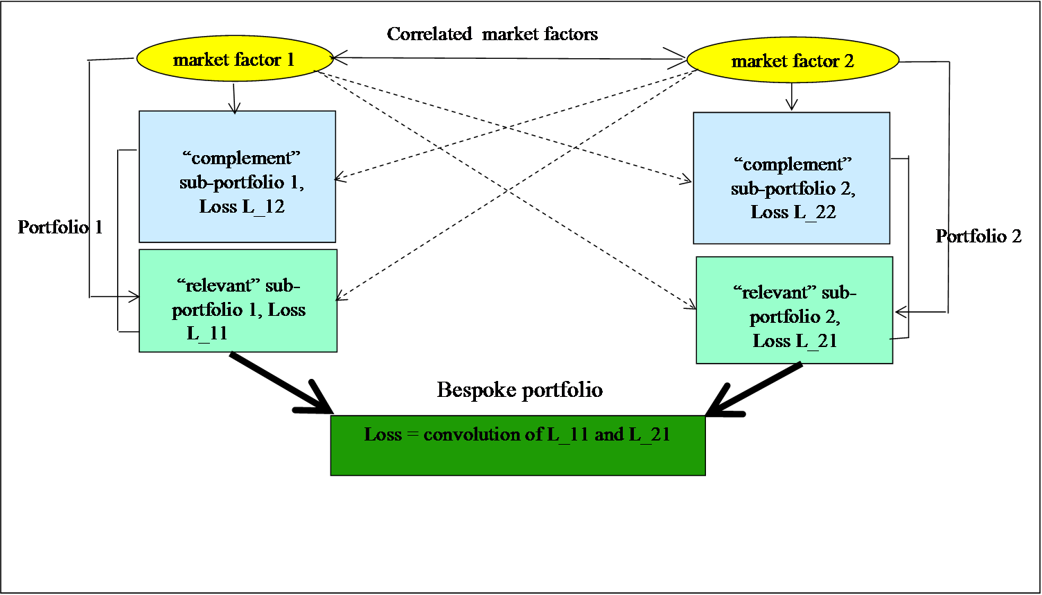
Figure 2: Layout of the Implied Multi-Factor Model (IMFM).

A two-factor framework thus seems to provide a minimal complexity level for a bespoke model needed for all but simplest bespoke portfolios that only need to be mapped onto one credit index. Given that market-implied prices of standard index tranches contain virtually no information on factors corresponding to separate sectors beyound a single factor corresponding to a diversified credit index as a whole, we believe that a two-factor specification may simultaneously serve as the upper “complexity bound” for a bespoke model to be useful and manageable in practice. We therefore stick to a two-factor formulation in what follows, and leave generalization for Sect.5.

2.3 Types of bespokes that can be priced with IMFM

As mentioned above, we want to be able to price arbitrary bespoke tranches which, by nature of their composition, should be mapped onto more than one index portfolio. We achieve this by constructing a certain hierarchy of ”bespoke complexity”. We first address a simplest bespoke portfolio: a bespoke that is made of ”chunks” of index portfolios. Assume we have two index portfolios $\Pi_{1}$ and $\Pi_{2}$ corresponding e.g. to the CDX.NA.IG and iTraxx Europe Main credit portfolios. Our simplest bespoke portfolio is made of names making up certain sub-portfolios (hereafter “relevant” sub-portfolios) $\Pi_{11}$ and $\Pi_{21}$ of index portfolios, respectively, while all names from complement sets $\Pi_{12}=\Pi_{1}\backslash\Pi_{11}$ and $\Pi_{22}=\Pi_{2}\backslash\Pi_{21}$ will be collectively referred to as ”complement” sub-portfolios (see Fig. 2). We will refer to such bespokes made of names from two, three etc. indices as $I2,I3,\ldots$ portfolios. One example of a $I2$ portfolio would be a bespoke portfolio with 100 names with 50 US names from the CDX.NA.IG index portfolio, and 50 European names from iTraxx Europe index portfolio.

Analysis in the following Sects. 3 and 4 will concentrate on the pricing of $I2$-type bespoke portfolios. This setting forms our basic case which will be worked out in great details. Treatment of more complex bespoke portfolios (e.g. portfolios made of chunks of three and more indices, or portfolios containing names not belonging to any index) will be presented as suitable generalizations of our basic setting in Sect.5.

2.4 Other applications: credit exotics and CVA on bespoke tranches

In addition to the ability to price bespoke CDO tranches on portfolios mapped onto more than one credit index, our model has, for its dynamic version, other interesting applications as well. First, more exotic portfolio derivatives, such as e.g. tranche options or forward-starting tranches, can be priced using a loss lattice with a backward recursion method, similar to how it is done in the BSLP model [2]. Second, the dynamic version of our multi-factor framework can be used for counterparty risk management of CDO tranches, in particular, for calculation of credit valuation adjustments (CVAs) on bespoke tranches. Again, a lattice formulation enables a quick and efficient implementation of the computational algorithm for this case.

2.5 Computational efficiency: a top-down approach

A multi-factor credit portfolio model of a traditional buttom-up type can run into numerical challenges rather quickly. Indeed, in consistent models for tranche prices such as RFL (which is a single-factor model), calibration takes around 5-30 min, depending on the model, efficiency of implementation and the particular calibration dataset. When moving to a two-factor framework with a double number of names, calibration time is expected to grow by at least an order of magnitude , which might become computationally infeasible on a single PC.

We choose to address these potential issues by adopting a version of the top-down approach to credit portfolios modeling. To introduce our setting, let us return to the case of a simplest $I2$-portfolio of the previous section. Recall that this is a bespoke composed of two ”chunks” of two index portfolios (out of the total of four ”chunks”). Let $X_{11}$ and $X_{21}$ be stochastic losses for ”relevant” sub-portfolios $\Pi_{11}$ and $\Pi_{21}$, respectively, with $X_{12}$ and $X_{22}$ being losses in complement sub-portfolios $\Pi_{12}=\Pi_{1}\backslash\Pi_{11}$ and $\Pi_{22}=\Pi_{2}\backslash\Pi_{21}$. Then we have the following obvious relations for the total losses $X_{1}$ and $X_{2}$ for portfolios $\Pi_{1}$ and $\Pi_{2}$:

$$X_{1}=X_{11}+X_{12}\;\;,\;\;X_{2}=X_{21}+X_{22}$$ (5)

The top-down specification of our approach amounts to the fact we only keep track of cumulative sub-portfolio losses $\vec{X}_{1}=\left(X_{11},X_{12}\right)$ and $\vec{X}_{2}=\left(X_{21},X_{22}\right)$ (we use hereafter a compact vector notation) , but not default states of individual names in either the ”relative” or ”complement” sub-portfolios. As long as the composition of our bespoke is as described above, the joint distribution of sub-portfolio losses $X_{11}$ and $X_{21}$ is all we need to price the bespoke.

The latter is easy to demonstrate. Consider a given time horizon $T$, and assume for the moment that we have somehow managed to calibrate this market factor distribution together with conditional joint loss distributions of sub-portfolios of the index portfolios $P_{1}\left(X_{11},X_{12}|\vec{Z}\right)$ and $P_{2}\left(X_{21},X_{22}|\vec{Z}\right)$ for this horizon. We can now easily price any tranche referencing the bespoke portfolio $\Pi_{B}=\Pi_{11}\cup\Pi_{21}$. Indeed, as losses in two portfolios are conditionally independent, the conditional loss distribution is easily found by convolution

$$P^{B}(X_{11}+X_{21}=x|\vec{Z})=\int dy\,P_{1}\left(y|\vec{Z}\right)P_{2}\left(x-y|\vec{Z}\right)$$ (6)

where conditional loss distributions $P_{1}\left(X_{11}|\vec{Z}\right)$ and $P_{2}\left(X_{21}|\vec{Z}\right)$ are obtained by marginalization of $P_{1}\left(X_{11},X_{12}|\vec{Z}\right)$ and $P_{2}\left(X_{21},X_{22}|\vec{Z}\right)$ over $X_{12}$ and $X_{22}$, respectively. Assuming that the common market factor is a continuous random variable with pdf $P_{Z}(\vec{z})$, the unconditional loss distribution is then obtained as follows:

$$p^{B}(x,T)=\int P^{B}(x|\vec{z})P_{Z}(\vec{z})d\vec{z}$$ (7)

Once the loss distribution for the bespoke portfolio is calculated on a grid $\{T_{i}\}$ of time horizons, any bespoke tranche is priced by standard formulae using numerical integration, see below in Sect.3.3.

3 IMFM in a single-period setting

In this section we present the Implied Multi-Factor Bespoke Model (IMFM) in a simplified single-period setting, where we only deal with the losses of index portfolios and their sub-portfolios at a single time horizon $T$. Once worked out, this will serve as a seed for a dynamic multi-period extension which is introduced in the next section.

3.1 A two-factor CreditMetrics prior

As was mentioned above, while our formulation is straightforward to generalize to an arbitrary number of market factors, our basic formulation will deal with a specific case of two market factors. In component notation, the latent variable for the $i$-th obligor in the $k$-th index portfolio takes the following form

$$A_{i}^{(k)}=\beta_{i1}^{(k)}Z_{1}+\beta_{i2}^{(k)}Z_{2}+\sqrt{1-\left(\beta_{i1}^{(k)}\right)^{2}-\left(\beta_{i2}^{(k)}\right)^{2}-2\rho\beta_{i1}^{(k)}\beta_{i2}^{(k)}}\varepsilon_{i}$$ (8)

Here $Z=(Z_{1},Z_{2})$ is a two-dimensional Gaussian random variable with means 0, variances of one, and correlation $\rho$.

While parameters of such model can be estimated from time series of spreads or defaults, we leave this task for future work, and instead adopt in this paper a simple parametrization that ensures consistency with a one-factor Gaussian copula framework. Assuming that the latter model is already estimated, our parametrization guarantees that no further work for parameter estimation is required.

We concentrate on a basic setting of two index portfolios, $\Pi_{1}$ and $\Pi_{2}$. We assume that

$$\beta_{i2}^{(1)}=\alpha\beta_{i1}^{(1)}\;\;,\;\;\beta_{i1}^{(2)}=\alpha\beta_{i2}^{(1)}$$ (9)

In words, we assume that for each name, its factor loading to the ”foreign” factor is a fixed proportion of its factor loading to its ”domestic” factor. It is easy to see that, as long as we view portfolio $\Pi_{1}$ ( $\Pi_{2}$) in isolation from portfolio $\Pi_{2}$ (resp. $\Pi_{1}$), the resulting model is identical to a one-factor model with factor loadings $b_{i}^{(1)}$ (or $b_{i}^{(2)}$) provided we set

$$\beta_{i1}^{(1)} = \frac{b_{i}^{(1)}}{\sqrt{1+2\alpha\rho+\alpha^{2}}}$$

$$\beta_{i2}^{(2)} = \frac{b_{i}^{(2)}}{\sqrt{1+2\alpha\rho+\alpha^{2}}}$$ (10)

Note that this framework slightly generalizes a more conventional hierarchical structure which is recovered with the present formalism in the limit $\alpha=0$.

Our parametrization (9) ensures that pairwise asset correlations for names in the same portfolio are the same as in the one-factor model irrespective of values of $\rho$ and $\alpha$, e.g. for portfolio $\Pi_{1}$ we obtain

$$\rho_{ij}^{(11)}=\beta_{i1}^{(1)}\beta_{j1}^{(1)}(1+2\alpha\rho+\alpha^{2})=b_{i}^{(1)}b_{j}^{(1)}$$ (11)

On the other hand, for two names in different portfolios we find

$$\rho_{ij}^{(12)}=\beta_{i1}^{(1)}\beta_{j2}^{(2)}(\rho(1+\alpha^{2})+2\alpha)=b_{i}^{(1)}b_{j}^{(2)}\frac{(1+\alpha^{2})\rho+2\alpha}{1+\alpha^{2}+2\alpha\rho}\geq\rho b_{i}^{(1)}b_{j}^{(2)}$$ (12)

Note that equality in the last expression follows in the limit $\alpha=0$ corresponding to a hierarchical model. Therefore, for a fixed $\rho$, a non-zero value $\alpha>0$ enhances inter-sector correlations.

In the implementation of the model, we discretize the market factor as follows. Using vector notation $\vec{Z}=\left(Z_{1},Z_{2}\right)$, the range of possible values of $\vec{Z}$ is discretized to a 2D grid

$$\vec{Z}_{\vec{m}}=\left(z_{m_{1}},z_{m_{2}}\right)$$ (13)

where $m_{1}=1,\ldots,N_{m1}$ and $m_{2}=1,\ldots,N_{m2}$, and

$$\vec{m}=\left(m_{1},m_{2}\right)\;,\;\;m_{1},m_{2}\in Z^{+}$$ (14)

is a 2D vector of integers. Corresponding discretized probabilities of realizations of these values of the market factor on the grid $\left\{z_{m_{1}},z_{m_{2}}\right\}$ read

$$h_{\vec{m}}\equiv h_{m_{1},m_{2}}=P\left[Z_{1}=z_{m_{1}},Z_{2}=z_{m_{2}}\right]=P\left[\vec{Z}=\vec{Z}_{\vec{m}}\right]$$ (15)

The difference the prior and “true” discretized market factor distributions thus amounts to different choice for weights $\{h_{\vec{m}}\}$. In the numerical examples to follows, we use a low number (between 10 and 20) of discretization points for each factor.

3.2 IMFM calibration via minimization of KL-divergence

Our problem is to calculate the joint distribution of the 6 random variables $\left(\vec{Z},\vec{X}_{1},\vec{X}_{2}\right)$ which is implied by the observed set of tranche price quotes. More exactly, we calibrate our model to a set of tranche expected losses at different maturities, which are obtained from market tranche prices using an arbitrage-free interpolation method. For the latter, one option is to use a spline-based method where no-arbitrage conditions are enforced as constraints, or using a top-down model such as BSLP [2] that does such interpolation internally. We do not expand on this procedure here, and instead refer the reader to the literature.

The implied joint distribution of $\left(\vec{Z},\vec{X}_{1},\vec{X}_{2}\right)$ is calculated as a minimal distortion (in the sense of information entropy, see below) of a ”prior” distribution (see below for possible choices for the prior), with the distortion just sufficient in order to match a given set of tranche expected losses $EL_{ki}$ , where $i=1,2$ stands for the credit index portfolio, and $k=1,\ldots,N_{i}$ enumerates tranches referencing the $i$-th portfolio. In information theory (see e.g. [6]), the ”distance”-type measure for two continuous distributions of a random variable $Y$ with densities $P_{1}(y)$ and $P_{2}(y)$ is given by the celebrated Kullback-Leibler relative entropy (KL-divergence)

$$D\left[P_{2}||P_{1}\right]=\int dyP_{2}(y)\log\frac{P_{2}(y)}{P_{1}(y)}$$ (16)

It can be easily checked using Jensen’s inequality that $D[P_{2}||P_{1}]$ is non-negative for all pairs $\left(P_{1},P_{2}\right)$, and reaches zero only when $P_{2}=P_{1}$. Note that for discrete distributions, integration in (16) should be substituted by summation. Having this in mind, in what follows we will keep for a while the continuous notation even for discrete distributions.

In our setting, variable $y$ appearing in (16) is 6-dimensional (6D):

$$Y=\left(\vec{Z},\vec{X}_{1},\vec{X}_{2}\right)\equiv\left(\vec{Z},\vec{X}\right)$$ (17)

where $\vec{X}=\left(\vec{X}_{1},\vec{X}_{2}\right)$ is a 4D vector storing all sub-portfolio losses in both index portfolios. The generalized KL-divergence for multi-dimensional distributions takes the same form as (16), provided integration (or summation) is extended over the whole $D$-dimensional space.

In what follows we assume that we pick a particular ”prior” model $Q$ for the joint risk-neutral distribution of $\left(\vec{Z},\vec{X}_{1},\vec{X}_{2}\right)$:

$$Q=Q\left(\vec{Z},\vec{X}_{1},\vec{X}_{2}\right)=Q\left(\vec{Z},\vec{X}\right)$$ (18)

We note that a few choices for the latter are popular among practitioners. One option is to use a uniform prior distribution corresponding to the state of maximum uncertainty about the value of $Y$. Another, and often more attractive choice is to use a prior measure corresponding to a specific parametric model. We will adopt a 2D Gaussian copula model with factor loadings defined as in (9) and (3.1) as the prior model in our approach.

Following the Minimum Cross-Entropy Method (MCE), we seek an implied joint risk-neutral distribution $P\left(\vec{Z},\vec{X}\right)$ that minimizes the KL-divergence between the “true” distribution $P\left(\vec{Z},\vec{X}\right)$ and the prior distribution $Q\left(\vec{Z},\vec{X}\right)$:

$$D\left[P\left(\vec{Z},\vec{X}\right)||Q\left(\vec{Z},\vec{X}\right)\right]=\int d\vec{Z}d\vec{X}P\left(\vec{Z},\vec{X}\right)\log\frac{P\left(\vec{Z},\vec{X}\right)}{Q\left(\vec{Z},\vec{X}\right)}$$ (19)

(here $d\vec{X}=\prod_{i=1,2}d\vec{X}_{i}$, and we use the integral notation for summation over the possible values of $\vec{Z}$), subject to pricing constraints

$$\int d\vec{Z}d\vec{X}P\left(\vec{Z},\vec{X}\right)F_{ik}\left(\vec{X}\right)=EL_{ik}\;,\;\;i=1,2\;,\;k=1\ldots,N_{i},N_{i}+1,N_{i}+2$$ (20)

where for a given $i$, the first $k=1,\ldots,N_{i}$ components of the generalized payoff functions $F_{ik}\left(\vec{X}\right)$ stand for the payoffs of the $k$-th tranche referencing the $i$-th index portfolio, while the last $(N_{i}+1)$-th and $(N_{i}+2)$-th components correspond to the payoffs (total expected losses) for sub-portfolios $\Pi_{i1}$ and $\Pi_{i2}$, respectively:

$$F_{ik}(\vec{X})=\left\{\begin{array}[]{lll}(X_{i1}+X_{i2}-K_{i,k-1})^{+}-(X_{i1}+X_{i2}-K_{ik})^{+}&\mbox{$k=1,\ldots,N_{i}$}\\ X_{i1}&\mbox{$k=N_{i}+1$}\\ X_{i2}&\mbox{$k=N_{i}+2$}\end{array}\right.$$ (23)

where $\{K_{ik}\}$ is a set of standard strikes for the $i$-th index portfolio. Generalized expected losses $EL_{ik}$ are defined using a similar convention. Eqs.(20) plus the normalization condition $\int d\vec{Z}d\vec{X}P\left(\vec{Z},\vec{X}\right)=1$ constitute the full set of constraints imposed in our model.

We follow the factor framework, i.e. we assume that $\vec{Z}$ is an unobservable ”market” factor such that conditional on the value of $\vec{Z}=\vec{Z}_{\vec{m}}$, all individual defaults in both index portfolios $\Pi_{1}\,,\Pi_{2}$ become independent. Correspondingly, the joint probability of $\left(\vec{Z}_{\vec{m}},\vec{X}\right)$ can be written as a product of the ”market factor” probabilities $h_{\vec{m}}$ (see Eq.(15)) and conditional loss distributions $P_{i}\left(\vec{X}_{i}|\vec{m}\right)\equiv P_{i}\left(\vec{X}_{i}|\vec{Z}=\vec{Z}_{\vec{m}}\right)$ ($i=1,2$) of losses in two index portfolios:

$$P\left(\vec{Z}=\vec{Z}_{\vec{m}},\vec{X}\right)=h_{\vec{m}}P\left(\vec{X}|\vec{m}\right)=h_{\vec{m}}\prod_{i=1,2}P_{i}\left(\vec{X}_{i}|\vec{m}\right)$$ (24)

Similarly, we write the prior model in the factor form:

$$Q\left(\vec{Z}=\vec{Z}_{\vec{m}},\vec{X}\right)=g_{\vec{m}}Q\left(\vec{X}|\vec{m}\right)=g_{\vec{m}}\prod_{i=1,2}Q_{i}\left(\vec{X}_{i}|\vec{m}\right)$$ (25)

Substituting (24), (25) into (19), the KL-divergence can be written as follows:

$$D\left[P\left(\vec{Z},\vec{X}\right)||Q\left(\vec{Z},\vec{X}\right)\right]=\sum_{\vec{m}}h_{\vec{m}}\log\frac{h_{\vec{m}}}{g_{\vec{m}}}+\sum_{i=1,2}\sum_{\vec{m}}h_{\vec{m}}\int d\vec{X}_{i}P_{i}\left(\vec{X}_{i}|\vec{m}\right)\log\frac{P_{i}\left(\vec{X}_{i}|\vec{m}\right)}{Q_{i}\left(\vec{X}_{i}|\vec{m}\right)}$$ (26)

The problem of minimization of the KL-divergence of distributions $P\left(\vec{Z},\vec{X}\right)$ and $Q\left(\vec{Z},\vec{X}\right)$ subject to constraints (20) can be solved in one of two ways. The first one is a direct functional minimization of KL-divergence in form (19) viewed as a functional of the joint probability $P\left(\vec{m},\vec{X}\right)=P\left(\vec{Z}_{\vec{m}},\vec{X}\right)$. The second, and equivalent, way is to use the expression (26) and minimize it jointly by viewing it as a functional of a priori independent distributions $h_{\vec{m}}$ and $P_{i}\left(\vec{X}|\vec{m}\right)$.

It is instructive to start with the second approach. We pose the variational optimization problem with the following Lagrangian functional:

$$\mathcal{L}^{\prime} = \sum_{\vec{m}}h_{\vec{m}}\log\frac{h_{\vec{m}}}{g_{\vec{m}}}+\sum_{i,\vec{m}}h_{\vec{m}}\int d\vec{X}_{i}\,P_{i}\left(\vec{X}_{i}|\vec{m}\right)\log\frac{P_{i}\left(\vec{X}_{i}|\vec{m}\right)}{Q_{i}\left(\vec{X}_{i}|\vec{m}\right)}$$ (27)

$$+ \sum_{i,k}\frac{1}{2\sigma_{ik}^{2}}\left(\sum_{\vec{m}}h_{\vec{m}}\int d\vec{X}_{i}\,P_{i}\left(\vec{X}_{i}|\vec{m}\right)F_{ik}(\vec{X})-EL_{ik}\right)^{2}$$

which should be minimized with respect to $h_{\vec{m}}$, $P_{1}\left(\vec{X}_{1}|\vec{m}\right)$ and $P_{2}\left(\vec{X}_{2}|\vec{m}\right)$. Here the first two terms enforce minimization of the KL-divergence between the “true” and prior joint distributions of the market factor and losses, while the last term enforces matching the tranche pricing data in the least square sense.

Note the relative importance of matching the data versus minimization of the KL “distance” to the prior distribution is controlled by parameters $\sigma_{i}$. In particular, when these parameters are large, the “true” distribution is very close to the prior, while the quality of fit is poor. In the opposite limit $\sigma_{i}\rightarrow 0$, one imposes an exact matching of pricing constraints. In this limit, the suitable Lagrangian reads, instead of (27),

$$\mathcal{L}^{\prime} = \sum_{\vec{m}}h_{\vec{m}}\log\frac{h_{\vec{m}}}{g_{\vec{m}}}+\sum_{i,\vec{m}}h_{\vec{m}}\int d\vec{X}_{i}\,P_{i}\left(\vec{X}_{i}|\vec{m}\right)\log\frac{P_{i}\left(\vec{X}_{i}|\vec{m}\right)}{Q_{i}\left(\vec{X}_{i}|\vec{m}\right)}$$ (28)

$$+ \sum_{i,k}\lambda_{ik}\left(\sum_{\vec{m}}h_{\vec{m}}\int d\vec{X}_{i}\,P_{i}\left(\vec{X}_{i}|\vec{m}\right)F_{ik}(\vec{X})-EL_{ik}\right)$$

where $\lambda_{ik}$ are Lagrange multipliers. While such formulation corresponds to a more conventional version of the MCE/MaxEnt methods, it may potentially lead to unstable calibration and overfitting, or even to no solution at all if constraints are incompatible. We therefore prefer the “soft constraint” version (27), where a compromise between robustness and quality of fit is expected to be achieved for some intermediate values of $\sigma_{i}$.

Unlike the “classical” MCE setting (28), a straightforward functional optimization of Lagrangian (27) is diffucult because of its non-linearity. Fortunately, a simple method is available that allows one to get rid of these non-linearities at the price of introducing auxiliary variables. Following Ref.[11], we consider the following modified Lagrangian

$$\mathcal{L} = \sum_{\vec{m}}h_{\vec{m}}\log\frac{h_{\vec{m}}}{g_{\vec{m}}}+\sum_{i,\vec{m}}h_{\vec{m}}\int d\vec{X}_{i}\,P_{i}\left(\vec{X}_{i}|\vec{m}\right)\log\frac{P_{i}\left(\vec{X}_{i}|\vec{m}\right)}{Q_{i}\left(\vec{X}_{i}|\vec{m}\right)}$$ (29)

$$+ \sum_{i,k}\frac{1}{2\sigma_{ik}^{2}}U_{ik}^{2}+\sum_{i,k}\lambda_{ik}\left(U_{ik}-\sum_{\vec{m}}h_{\vec{m}}\int d\vec{X}_{i}\,P_{i}\left(\vec{X}_{i}|\vec{m}\right)F_{ik}(\vec{X})+EL_{ik}\right)$$

It is easy to see that this modified Lagrangian is equivalent to the original one (27) if, in addition to minimization with respect to distributions $h_{\vec{m}}$, and $P_{1}\left(\vec{X}_{i}|\vec{m}\right)$ ( $i=1,2$), we also vary it with respect to parameters $U_{ik}$ and $\lambda_{ik}$. Indeed, if we first optimize (28) with respect to $\lambda_{ik}$, we obtain

$$U_{ik}=\sum_{\vec{m}}h_{\vec{m}}\int d\vec{X}_{i}\,P_{i}\left(\vec{X}_{i}|\vec{m}\right)F_{ik}(\vec{X})-EL_{ik}$$ (30)

and back substitution in (29) leads to (27). The same result is obtained if we optimize wrt $U_{ik}$ first, and $\lambda_{ik}$ next.

Having established equivalence of (29) and (27), we now want to proceed differently with (29). We start with minimization with respect to $P_{1}\left(\vec{X}_{1}|\vec{m}\right)$ and $P_{2}\left(\vec{X}_{2}|\vec{m}\right)$. We find

$$P_{i}\left(\vec{X}_{i}|\vec{m}\right) = \frac{1}{Z_{i}(\vec{m},\lambda)}Q_{i}\left(\vec{X}_{i}|\vec{m}\right)e^{\sum_{k}\lambda_{ik}\left(F_{ik}(\vec{X}_{i})-EL_{ik}\right)}\;,\;\;i=1,2$$

$$Z_{i}(\vec{m},\lambda) = \int d\vec{X}_{i}\,Q_{i}\left(\vec{X}_{i}|\vec{m}\right)e^{\sum_{k}\lambda_{ik}\left(F_{ik}(\vec{X}_{i})-EL_{ik}\right)}$$ (31)

Interestingly, Eqs.(3.2) indicate that even though we start with the factorized prior distributions $Q_{i}\left(\vec{X}_{i}|\vec{m}\right)=Q_{i1}\left(X_{i1}|\vec{m}\right)Q_{i2}\left(X_{i2}|\vec{m}\right)$, we end up with non-factorizable conditional distributions $P_{i}\left(\vec{X}_{i}|\vec{m}\right)$ due to the fact that payoff functions $F_{ik}$ depend on the sums $X_{i1}+X_{i2}$ non-linearly. As discussed in details in Appendix, this both makes sense intuitively and can be explained within Information Theory. Therefore, while for the prior model losses in all four sub-portfolios $\Pi_{11},\Pi_{12},\Pi_{21}$ and $\Pi_{22}$ were independent conditional on the market factor, as a result of calibration, they become dependent within the same parent index portfolio, while retaining independence across different index portfolios.

Let us now proceed with the solution of optimization problem (27). Substituting (3.2) back in the Lagrangian (29), we obtain

$$\mathcal{L}=\sum_{\vec{m}}h_{\vec{m}}\log\frac{h_{\vec{m}}}{g_{\vec{m}}}-\sum_{\vec{m}}h_{\vec{m}}\sum_{i=1,2}\log Z_{i}(\vec{m},\lambda)+\sum_{i,k}\left(\frac{1}{2\sigma_{ik}^{2}}U_{ik}^{2}+\lambda_{ik}U_{ik}\right)$$ (32)

Minimizing this with respect to $h_{\vec{m}}$, we find

$$h_{\vec{m}} = \frac{1}{Z(\lambda)}g_{\vec{m}}\prod_{i=1,2}Z_{i}(\vec{m},\lambda)$$

$$Z(\lambda) = \sum_{\vec{m}}g_{\vec{m}}\prod_{i=1,2}Z_{i}(\vec{m},\lambda)$$ (33)

Minimization of (32) with respect to $U_{ik}$ gives

$$U_{ik}=-\lambda_{ik}\sigma_{ik}^{2}$$ (34)

We next substitute the extremal values (3.2) and (34) into (32) to obtain

$$\mathcal{L}=-\log Z(\lambda)-\frac{1}{2}\sum_{ik}\lambda_{ik}^{2}\sigma_{ik}^{2}$$ (35)

The values of Lagrange multipliers should now be found numerically by maximization of (35), or equivalently, minimization of the Lagrangian

$$\mathcal{L^{\prime}}(\lambda)=\log Z(\lambda)+\frac{1}{2}\sum_{ik}\lambda_{ik}^{2}\sigma_{ik}^{2}$$ (36)

This is a convex optimization problem as the matrix of second derivatives is given by the covariance matrix of constraints

$$\frac{\partial^{2}\mathcal{L^{\prime}}}{\partial\lambda_{ik}\lambda_{jl}}=\langle F_{ik}F_{jl}\rangle-\langle F_{ik}\rangle\langle F_{jl}\rangle+\delta_{ij}\delta_{kl}\sigma_{ik}^{2}=cov(F_{ik},F_{jl})+\delta_{ij}\delta_{kl}\sigma_{ik}^{2}$$ (37)

which is a positive-definite matrix. Therefore the solution is unique if it exists.

Once the Lagrange multipliers are found, the solution of the problem is given by Eqs.(3.2) and (3.2), and the unconditional loss distribution for the bespoke portfolio is calculated using Eqs.(6) and (7).

3.3 Pricing bespoke CDO tranches

The analysis of the previous section applies to a given single time horizon $T$. To price tranches referencing a given bespoke portfolio, we need to pick a time grid $\{T_{i}\}$. For each node on this grid, we find implied dichotomic index loss distributions for both reference indices as described above, and then calculate the implied loss distribution $p^{B}(x,T_{i})$ for the bespoke as outlined in Sect.2.4, see Eq.(7). After that, tranches on the bespoke CDO are priced using standard formulae that we provide here for completeness.

Let $K_{d},K_{u}$ be detachment/attachment points of the bespoke tranche. The term structure of tranche expected losses is then calculated as follows

$$EL_{T_{i}}\equiv EL_{i}=\frac{1}{K_{u}-K_{d}}\int dx\,p^{B}(x,T_{i})\left[\left(x-K_{d}\right)^{+}-\left(x-K_{u}\right)^{+}\right]$$ (38)

The default leg (otherwise known as contingent leg) of the tranche is given by

$$\mathcal{D}=N_{0}\int_{0}^{T}B(0,t)dEL_{t}\simeq N_{0}\sum_{i=1}^{M}\frac{1}{2}\left(B_{i-1}+B_{i}\right)(EL_{i}-EL_{i-1})$$ (39)

where $B(0,t)$ is a risk-free discount factor.

The premium leg (paid by the protection buyer to the protection seller) is given by

$$\mathcal{P}(S) = S\cdot N_{0}\sum_{i=1}^{M}\Delta_{i}\left(B_{i}\cdot EN_{T_{i}}-\int_{T_{i-1}}^{T_{i}}\frac{t-T_{i-1}}{T_{i}-T_{i-1}}B(0,t)dEN_{t}\right)$$

$$\simeq S\cdot N_{0}\sum_{i=1}^{M}\Delta_{i}B_{i}\frac{1}{2}\left(EN_{i-1}+EN_{i}\right)$$

where $S$ is the tranche spread, $\Delta_{i}$ is the day count fraction, and

$$EN_{i}\equiv EN_{T_{i}}=1-EL_{i}$$ (41)

is the expected tranche outstanding notional at time $T_{i}$. The integral term in (3.3) represents the accrued coupon due to defaults happening between the coupon payments dates. The integral is calculated using the standard approximation (see e.g. [19]) that amounts to substitution of $(t-T_{i-1})/(T_{i}-T_{i-1})$ and $B(0,t)$ by 1/2 and $B_{i}$, respectively. The fair (break-even) tranche par spread, $S$, is determined from the par equation $\mathcal{D}=\mathcal{P}(S)$.

3.4 Discussion

3.4.1 Inter-temporal consistency and time arbitrage

The framework presented so far corresponds to what is known as “single-period” models in the literature. In this approach, one deals only with marginal loss distributions at a given set of maturities, but not with joint probabilities of losses at different time horizons. Note that the knowledge of marginal loss distributions is sufficient for pricing of CDO tranches. Reversing this argument, one can state that market prices of index tranches contain information on marginal loss distributions but not on joint inter-temporal distributions, see e.g. [2] for a related discussion.

In the above framework, we treat different time horizons separately from each other, and calculate the implied distribution that matches a set of tranche expected losses (ELs) for each node $T_{i}$ on a time grid. If the set of input tranche ELs is arbitrage-free across both strikes and time, then the resulting implied distribution will be free of arbitrage across time for loss levels corresponding to strikes in the calibration set. However, no-arbitrage across time is not guaranteed in this approach for other loss levels.

While we have not encountered violations of time arbitrage in practice with our numerical experiments, the above implies that it may happen. Note that by continuity, once we calibrate to an arbitrage-free set of tranche ELs, the time no-arbitrage holds not only for reference strikes, but also for loss values around these strikes. Therefore, a simple practical way to prevent volation of time arbitrage is to increase the number of strikes in the calibration set.

A more principled approach to the problem of possible time arbitrage requires switching to a dynamic framework. Similar to the way no-arbitrage across strikes is guaranteed by the properties of the KL-divergence (see above in Sec.2.1), no-arbitrage across time is ensured once we pick an arbitrage-free prior model for transition probabilities. Such a construction will be presented in Sect.4.

3.4.2 What form of entropy minimization should one use?

A couple of further comments are in order here. First, note that Eqs.(3.2) and (3.2) imply the following form of the ”true” (”posterior”) joint distribution $P\left(\vec{m},\vec{X}\right)$:

$$P\left(\vec{X},\vec{Z}_{\vec{m}}\right)=h_{\vec{m}}\prod_{i=1,2}P\left(\vec{X}_{i}|\vec{m}\right)=\frac{1}{Z(\lambda)}Q\left(\vec{X},\vec{Z}_{\vec{m}}\right)e^{\sum_{i,k}\lambda_{ik}\left(F_{ik}(\vec{X})-EL_{ik}\right)}$$ (42)

which could equivalently be obtained by a direct minimization of the KL-divergence in the form (19), subject to constraints (20). This would provide a much shorter derivation of our final result (3.2), (3.2). This is required, of course, for self-consistency of the method.

Second, the lengthy derivation leading to our equations (3.2), (3.2) was given above with the intent to illustrate the modelling freedom in the implied loss approaches which have recently become popular in the literature on credit portfolio modeling. Assume for the moment that instead of independent variation of (26) with respect to both market factor distribution $h_{\vec{m}}$ and conditional loss distributions $P_{i}\left(\vec{X}_{i}|\vec{m}\right)$, we would fix the functional form of, say, the latter, and only optimize with respect to the former (see e.g. in Rosen and Saunders [20]). It is clear from the above derivation that such a procedure would yield a sub-optimal (in the sense of KL-divergence) solution for the joint distribution of the market factor and sub-portfolio losses.

The latter point is easy to illustrate a bit more formally. Assume, for the sake of argument, that we calibrate to a set of tranche expected losses for synthetic first loss (equity) tranches with payoff functions $F_{ik}(x)=\min\left(x,K_{k}\right)$. Assume that we fix the conditional loss distributions to their prior form, $P_{i}\left(\vec{X}_{i}|\vec{m}\right)=Q_{i}\left(\vec{X}_{i}|\vec{m}\right)$. In this case, minimization of the Lagrangian (27) with respect to $h_{\vec{m}}$ yields

$$h_{\vec{m}}=\frac{1}{\hat{Z}(\lambda)}g_{\vec{m}}e^{-\sum_{ik}\lambda_{ik}\left(\int d\vec{X}_{i}Q_{i}\left(\vec{X}_{i}|\vec{m}\right)F_{ik}(\vec{X}_{i})-EL_{ik}\right)}$$ (43)

where $\hat{Z}(\lambda)$ is a normalization factor, and Lagrange multipliers $\lambda_{ik}$ minimize the Lagrangian function

$$\hat{\mathcal{L}}^{\prime\prime}\equiv\log\hat{Z}(\lambda)=\log\left(\sum_{\vec{m}}g_{\vec{m}}\prod_{i=1,2}e^{-\sum_{k}\lambda_{ik}\left(\int d\vec{X}_{i}Q_{i}\left(\vec{X}_{i}|\vec{m}\right)F_{ik}(\vec{X}_{i})-EL_{ik}\right)}\right)$$ (44)

Comparing this Lagrangian to (36), we note that in the limit $\sigma_{i}\rightarrow 0$, they have the same gradients and hence reach their minima at the same point $\vec{\lambda}=\vec{\lambda}_{\star}$. On the other hand, as long as functions $e^{-\lambda_{ik}F_{ik}(x)}$ are convex in $x$, by Jensen’s inequality we have, for any fixed vector $\vec{\lambda}$:

$$\int d\vec{X}_{i}Q\left(\vec{X}_{i}|\vec{m}\right)e^{-\sum_{ik}\lambda_{ik}F_{ik}(\vec{X}_{i})}\leq e^{-\sum_{ik}\lambda_{ik}\int d\vec{X}_{i}Q_{i}\left(\vec{X}_{i}|\vec{m}\right)F_{ik}(\vec{X}_{i})}$$ (45)

which implies that the minimum of $\mathcal{L}^{\prime}$ lies lower than the minimum of $\mathcal{L}^{\prime\prime}$. This exactly means sub-optimality of the solution (43) in terms of KL-distance between the ”true” and ”prior” joint distributions of $\left(\vec{X}_{i},\vec{m}\right)$.

Finally, note that even though it might appear that allowing for independent variations of $h_{\vec{m}}$ and $P\left(\vec{X}_{i}|\vec{m}\right)$ brings ”too much flexibility” to the problem, this is not true: adjustments to both $h_{\vec{m}}$ and $P\left(\vec{X}_{i}|\vec{m}\right)$ are driven by the same set of Lagrange multipliers, and are equivalent to a single adjustment of the joint probability $P\left(\vec{Z}_{\vec{m}},\vec{X}\right)$, see (42). In the nomenclature of factor models, this means that the least biased distortion of a prior joint distribution $Q\left(\vec{X},\vec{Z}_{\vec{m}}\right)$ is obtained when both the market factor distribution and conditional loss distribution are allowed to vary. The joint optimization of distribution $Q\left(\vec{X},\vec{Z}\right)$ has the same complexity as optimization of the market factor distribution alone.

4 IMFM: a dynamic multi-period formulation

Here we present a dynamic generalization of the formalism of the previous section to a multi-period setting. We consider a (sufficiently dense) set of reference maturities $T_{0},T_{1},\ldots,T_{N_{T}-1}$. We set $T_{-1}=0$ to be today’s time. Let

$$\vec{X}_{i}^{n}=\left(X_{i1}(T_{n}),X_{i2}(T_{n})\right)\;,\;\;i=1,2\;,\;n=0,\ldots,N_{T}-1$$ (46)

be the loss in the $i$-th portfolio at time $t=T_{n}$, expressed as a tuple of losses in the ”relevant” and complement sub-portfolios at the same time, respectively. Alternatively, we use a dynamic 4D vector

$$\vec{X}^{n}=\left(\vec{X}_{1}(T_{n}),\vec{X}_{2}(T_{n})\right)$$ (47)

to specify the joint sub-portfolio losses in the two index portfolios at time $T_{n}$.

We assume a dynamic framework for the 2D common market factor $\vec{Z}_{t}=\left(Z_{1}(t),Z_{2}(t)\right)$, where the (time-dependent) components $Z_{1}(t),Z_{2}(t)$ take values on the same grid (13). Furthermore, we assume that $\vec{Z}_{t}$ is a right-continuous jump process with jumps allowed only at times $\{T_{n}\}$:

$$\vec{Z}_{t}=\vec{Z}^{n}=\left(Z_{1}(T_{n}),Z_{2}(T_{n})\right)\;,\;t\in[T_{n-1},T_{n}[\;,\;n=0,1,\ldots,N_{T}-1$$ (48)

Similar to (15), we introduce the time-dependent integer-valued 2D vector $\vec{m}^{n}$ that labels discrete states of the market factor components on the interval $[T_{n-1},T_{n}[$:

$$h_{\vec{m}^{n}}\equiv P\left(\vec{Z}(t)=\vec{Z}_{\vec{m}^{n}}\right)=P\left(Z_{1}(t)=z_{m_{1}},Z_{2}(t)=z_{m_{2}}\right)\;,\;t\in[T_{n},T_{n+1}[\;,\;n=0,1,\ldots,N_{T}-1$$ (49)

We assume a Markovian setting in our model, i.e. the state variables at time $T_{n}$ depend only on state variables at previous time $T_{n-1}$ but not on their prior history:

$$P\left(\vec{X}^{n},\vec{m}^{n}|\vec{X}^{0}\ldots,\vec{X}^{n-1},\vec{m}^{0},\ldots,\vec{m}^{n-1}\right)=P\left(\vec{X}^{n},\vec{m}^{n}|\vec{X}^{n-1},\vec{m}^{n-1}\right)$$ (50)

We now construct a multi-period generalization of the single-period setting of the previous section, where one infers transition probabilities $P\left(\vec{X}^{n},\vec{m}^{n}|\vec{X}^{n-1},\vec{m}^{n-1}\right)$ instead of marginal probabilities $P\left(\vec{X}^{n},\vec{m}^{n}\right)$. The model is constructed (equivalently, calibrated) within a bootstrap procedure in the time dimension, starting with the first maturity $T_{0}$. In treating the time dimension of the problem, our approach is similar to that developed in Ref.[11] in a somewhat different context of pricing equity derivatives.

4.1 The first maturity $T_{0}$

For the first maturity $T_{0}$, we assume that today ($t=0$, or equivalently $n=-1$) we have no losses in either portfolio, and the value of the market factor prior to time $T_{-1}$ is fixed somehow (this value is irrelevant for calculation of the joint law of $\vec{X}(t),\vec{m}(t)$ at time $t=T_{0}$). The marginal joint distribution $P\left(\vec{X}^{0},\vec{m}^{0}\right)$ is then calculated using the formalism of the previous section, see Eq.(42):

$$P\left(\vec{X}^{0},\vec{Z}_{\vec{m}^{0}}\right) = h_{\vec{m}^{0}}\prod_{i=1,2}P_{i}\left(\vec{X}_{i}^{0}|\vec{m}^{0}\right)=\frac{1}{Z_{0}(\lambda)}Q\left(\vec{X}^{0},\vec{Z}_{\vec{m}^{0}}\right)e^{\sum_{i,k}\lambda_{ik}\left(F_{ik}(\vec{X}^{0})-EL_{ik}^{0}\right)}$$

$$Z_{0}(\lambda) = \sum_{\vec{m}^{0}}g_{\vec{m}^{0}}\int d\vec{X}^{0}Q\left(\vec{X}^{0},\vec{Z}_{\vec{m}^{0}}\right)e^{\sum_{i,k}\lambda_{ik}\left(F_{ik}(\vec{X}^{0})-EL_{ik}^{0}\right)}$$ (51)

where $Q(\left(\vec{Z}_{\vec{m}^{0}},\vec{X}^{0}\right)$ is the prior joint distribution of the state variables at time $T_{0}$.

4.2 Further maturities $T_{n}$, $n=1,\ldots,N_{T}$

Now we assume that we have calculated the implied joint distribution for the previous maturity $T_{n-1}$, and we want to move one step on the time grid, i.e. calculate the transition probabilities $P\left(\vec{X}^{n},\vec{m}^{n}|\vec{X}^{n-1},\vec{m}^{n-1}\right)$. The latter should be calculated (calibrated) in a way that ensures consistency with pricing data for maturity $T_{1}$ as seen today, at time $t=0$.

Our method to calculate transition probabilities $P\left(\vec{X}^{n},\vec{m}^{n}|\vec{X}^{n-1},\vec{m}^{n-1}\right)$ is based on minimizing of a suitable KL-divergence, similar to the procedure used above in the single-period setting. The only difference from the previous case is that now we have to minimize the conditional cross entropy of transition probabilities $P\left(\vec{X}^{n},\vec{m}^{n}|\vec{X}^{n-1},\vec{m}^{n-1}\right)$ and $Q\left(\vec{X}^{n},\vec{m}^{n}|\vec{X}^{n-1},\vec{m}^{n-1}\right)$. The latter is defined as follows (see e.g. [6]):

$$D\left[P||Q\right]=\sum_{\vec{m}^{n-1},\vec{m}^{n}}\int d\vec{X}^{n-1}d\vec{X}^{n}P\left(\vec{X}^{n},\vec{m}^{n},\vec{X}^{n-1},\vec{m}^{n-1}\right)\log\frac{P\left(\vec{X}^{n},\vec{m}^{n}|\vec{X}^{n-1},\vec{m}^{n-1}\right)}{Q\left(\vec{X}^{n},\vec{m}^{n}|\vec{X}^{n-1},\vec{m}^{n-1}\right)}$$ (52)

which can be interpreted as the KL-divergence of transition probabilities $P\left(\vec{X}^{n},\vec{m}^{n}|\vec{X}^{n-1},\vec{m}^{n-1}\right)$ and $Q\left(\vec{X}^{n},\vec{m}^{n}|\vec{X}^{n-1},\vec{m}^{n-1}\right)$ viewed as a function of initial values $\vec{X}^{n-1},\vec{m}^{n-1}$, and averaged over these initial values using the marginal joint probability distribution $P\left(\vec{X}^{n-1},\vec{m}^{n-1}\right)$ calculated at the previous time step:

$$D\left[P||Q\right]=\sum_{\vec{m}^{n-1}}\int d\vec{X}^{n-1}P\left(\vec{X}^{n-1},\vec{m}^{n-1}\right)D(\vec{X}^{n-1},\vec{m}^{n-1})$$ (53)

Introducing transition probabilities for the market factors

$$h\left(\vec{m}^{n}|\vec{m}^{n-1},\vec{X}^{n-1}\right)=P\left[\vec{Z}^{n}=\vec{Z}_{\vec{m}^{n}}|\vec{Z}^{n-1}=\vec{Z}_{\vec{m}^{n-1}},\vec{X}^{n-1}\right]$$ (54)

and the corresponding prior probabilities

$$g\left(\vec{m}^{n}|\vec{m}^{n-1},\vec{X}^{n-1}\right)=P^{(prior)}\left[\vec{Z}^{n}=\vec{Z}_{\vec{m}^{n}}|\vec{Z}^{n-1}=\vec{Z}_{\vec{m}^{n-1}},\vec{X}^{n-1}\right]$$ (55)

the conditional KL-divergence (53) can be put in a more suggestive form (compare with (26)):

$$D\left[P||Q\right] = \sum_{\vec{m}^{n-1}}\int d\vec{X}^{n-1}P\left[\vec{X}^{n-1},\vec{m}^{n-1}\right]\left(\sum_{\vec{m}^{n}}h\left(\vec{m}^{n}|\vec{m}^{n-1},\vec{X}^{n-1}\right)\log\frac{h\left(\vec{m}^{n}|\vec{m}^{n-1},\vec{X}^{n-1}\right)}{g\left(\vec{m}^{n}|\vec{m}^{n-1},\vec{X}^{n-1}\right)}\right.$$ (56)

$$+ \left.\int d\vec{X}^{n}P\left(\vec{X}^{n}|\vec{m}^{n},\vec{X}^{n-1},\vec{m}^{n-1}\right)\log\frac{P\left(\vec{X}^{n}|\vec{m}^{n},\vec{X}^{n-1},\vec{m}^{n-1}\right)}{Q\left(\vec{X}^{n}|\vec{m}^{n},\vec{X}^{n-1},\vec{m}^{n-1}\right)}\right)$$

Our pricing constraints now take the following form:

$$\sum_{\vec{m}^{n-1}}\int d\vec{X}^{n-1}P\left(\vec{X}^{n-1},\vec{m}^{n-1}\right)\sum_{\vec{m}^{n}}\int d\vec{X}^{n}P\left(\vec{X}^{n},\vec{m}^{n}|\vec{X}^{n-1},\vec{m}^{n-1}\right)F_{ik}(\vec{X}^{n})=EL_{ik}^{n}$$ (57)

While the problem of minimization of (56) subject to constraints (57) admit more general priors, in what follows we restrict ourselves to a particular sort of priors. First we assume that prior transition probabilities for the market factor depend only on the previous value of the market factor but not on the previous loss level:

$$g\left(\vec{m}^{n}|\vec{m}^{n-1},\vec{X}^{n-1}\right)=g\left(\vec{m}^{n}|\vec{m}^{n-1}\right)$$ (58)

A possible candidate for the prior market factor transition matrix can be a simple birth-and-death discrete-time Markov chain.

Second, we assume that the probability of reaching loss $\vec{X}^{n}$ by the end of period $[T_{n-1},T_{n}[$ depends only on previous losses $\vec{X}^{n-1}$ and the value $\vec{m}^{n}$ of the market factor on this interval, but not on its previous value:

$$Q_{i}\left(\vec{X}_{i}^{n}|\vec{m}^{n},\vec{X}_{i}^{n-1},\vec{m}^{n-1}\right)=Q_{i}\left(\vec{X}_{i}^{n}|\vec{m}^{n},\vec{X}_{i}^{n-1}\right)$$ (59)

Within such reduced class of admissible priors, for the latter we can use simple single-period models such as a two-factor Gaussian copula (or the RFL model) that we used above in a static setting of Sect.3.

A brief inspection of Eqs.(56) and (57) establishes that the results of a corresponding Lagrangian optimization problem of minimization of (56) subject to constraints (57) can be immediately read off the previous formulae for a single-period case, provided all marginal probabilities should substituted by transition probabilities of transition from the previous state $\left(\vec{X}^{n-1},\vec{Z}^{n-1}\right)$. This observation allows one to immediately write down the result (which can of course be readily checked following steps similar to those described above for the single-period setting):

$$P_{i}\left(\vec{X}_{i}^{n}|\vec{m}^{n},\vec{X}_{i}^{n-1}\right) = \frac{1}{Z_{i\lambda}^{k}\left(\vec{m}^{n},\vec{X}_{i}^{n-1}\right)}Q_{i}\left(\vec{X}_{i}^{n}|\vec{m}^{n},\vec{X}_{i}^{n-1}\right)e^{\sum_{k}\lambda_{ik}\left(F_{ik}(\vec{X}_{i}^{n})-EL_{ik}^{n}\right)}$$

$$Z_{i\lambda}^{n}\left(\vec{m}^{n},\vec{X}_{i}^{n-1}\right) = \int d\vec{X}_{i}^{n}Q_{i}\left(\vec{X}_{i}^{n}|\vec{m}^{n},\vec{X}_{i}^{n-1}\right)e^{\sum_{k}\lambda_{ik}\left(F_{ik}(\vec{X}_{i}^{n})-EL_{ik}^{n}\right)}$$ (60)

$$h\left(\vec{m}^{n}|\vec{m}^{n-1},\vec{X}^{n-1}\right) = \frac{1}{\hat{Z}_{\lambda}^{n}\left(\vec{X}^{n-1},\vec{m}^{n-1}\right)}g\left(\vec{m}^{n}|\vec{m}^{n-1}\right)\prod_{i=1,2}Z_{i\lambda}^{n}\left(\vec{m}^{n},\vec{X}_{i}^{n-1}\right)$$

$$\hat{Z}_{\lambda}^{n}\left(\vec{m}^{n-1},\vec{X}^{n-1}\right) = \sum_{\vec{m}^{n}}g\left(\vec{m}^{n}|\vec{m}^{n-1}\right)Z_{1\lambda}^{n}\left(\vec{X}_{1}^{n-1},\vec{m}^{n}\right)Z_{2\lambda}^{n}\left(\vec{X}_{2}^{n-1},\vec{m}^{n}\right)$$

Note that the first of Eqs.(4.2) shows that our framework is arbitrage-free as long as the prior model is, irrespective of the model $g\left(\vec{m}^{n}|\vec{m}^{n-1}\right)$ for the dynamic market factor. Furthermore, the third of Eqs.(4.2) demonstrates that our model produces credit contagion: even though we started with a prior transition probabilities $g\left(\vec{m}^{n}|\vec{m}^{n-1}\right)$ that were independent of the previous loss levels $\vec{X}_{i}^{n-1}$, the “true” transition probabilities $h\left(\vec{m}^{n}|\vec{m}^{n-1},\vec{X}^{n-1}\right)$ do depend on them. Finally, note that Eqs.(4.2) can also be combined into a formula for joint transition probabilities

$$P\left(\vec{m}^{n},\vec{X}^{n}|\vec{m}^{n-1},\vec{X}^{n-1}\right)=\frac{1}{\hat{Z}_{\lambda}^{n}\left(\vec{m}^{n-1},\vec{X}^{n-1}\right)}Q\left(\vec{m}^{n},\vec{X}^{n}|\vec{m}^{n-1},\vec{X}^{n-1}\right)e^{\sum_{i,k}\lambda_{ik}\left(F_{ik}(\vec{X}_{i}^{n})-EL_{ik}^{n}\right)}$$ (61)

Here the values of Lagrange multipliers $\lambda_{ik}$ should be substituted by the solution of a $(N_{1}+N_{2}+4)$-dimensional convex optimization problem with the Lagrangian function (compare with Eq.(36))

$$\mathcal{L}=\sum_{\vec{m}^{n-1}}\int d\vec{X}^{n}P\left(\vec{m}^{n-1},\vec{X}^{n-1}\right)\log\hat{Z}_{\lambda}^{n}\left(\vec{m}^{n-1},\vec{X}^{n-1}\right)+\frac{1}{2}\sum_{ik}\lambda_{ik}^{2}\sigma_{ik}^{2}$$ (62)

4.3 Completing one step of time bootstrap

Having computed the transition probability $P\left[\vec{X}^{n},\vec{m}^{n}|\vec{X}^{n-1},\vec{m}^{n-1}\right]$ and using the marginal probability $P\left[\vec{X}^{n-1},\vec{m}^{n-1}\right]$ known from the previous time step, we know use them to calculate the marginal joint distribution of state variables at time $T_{k}$:

$$P\left(\vec{m}^{n},\vec{X}^{n}\right)=\sum_{\vec{m}^{n-1}}\int d\vec{X}^{n-1}P\left(\vec{m}^{n-1},\vec{X}^{n-1}\right)P\left(\vec{m}^{n},\vec{X}^{n}|\vec{m}^{n-1},\vec{X}^{n-1}\right)$$ (63)

Unless we reached the final maturity $T_{N_{k}}$ on the time grid, we know increment $k\rightarrow k+1$, coming up with a problem identical to that just solved for the previous period, where (63) plays the role of the marginal joint distribution from the previous step.

5 Generalizations

5.1 More market factors

Formally generalization to more than two market factors is straightforward and follows the same lines as developed above. However, for higher number of factors (three and more?) Monte Carlo may be preferred for integration over market factor distribution as well as for calculation of conditional loss distributions.

5.2 More index chunks in the bespoke

Assume that we have to price a tranche on a bespoke composed of three chunks belonging to three different indices $\{I_{i}\}_{i=1}^{3}$. Such calculation would proceed along the same line as described above, with a simultaneous calibration to tranches referencing all indices $I_{i}$, while the conditional loss distribution (6) would now be given by a two-dimensional convolution instead of a one-dimensional one. Note that for this case a three-factor version of the model may be preferred to a two-factor one.

5.3 Bespoke portfolios with “bespoke” names

So far, we have assumed that each name in a bespoke portfolio belongs to some credit index. In practice, this is often not the case, as majority of actual bespoke portfolios typically have some “bespoke” names, i.e. names that do not belong to any credit index.

Let us assume that we are given a bespoke portfolio of the following form: $\Pi_{B}=\Pi_{11}\cup\tilde{\Pi}_{21}$, where $\Pi_{11}$ stands for a sub-set of names from an index portfolio $I_{1}$ (e.g. CDX.NA.IG) and $\tilde{\Pi}_{21}$ is a sub-set of “bespoke” names that do not belong in any credit index. For example, the sub-set $\tilde{\Pi}_{21}$ can be composed of non-investment grade US names. In this case, we would take the CDX.NA.HY portfolio is the closest second benchmark security to our bespoke set.

More generally, assume that names in $\tilde{\Pi}_{21}$ are similar in terms of their geographic sectors and ratings to names in another index $I_{2}$. We can then pose (and solve) the problem of finding a sub-set $\Pi_{21}$ of names from $I_{2}$ that provides the best approximation of the set $\tilde{\Pi}_{21}$ in terms of sector diversification, average expected loss, and possibly higher moments of the loss distribution. This is a combinatorial optimization problem that can be solved e.g. using a genetic algorithm (details will be given elsewhere). Once such a proxy index sub-portfolio is found, our problem of pricing bespoke tranches can be reduced to the previous problem of pricing tranches on a $I2$-type bespoke portfolio.

The approximating sub-portfolio $\Pi_{21}$ is generally expected to have an average expected loss (EL) that is not exactly equal to the EL of the original set $\tilde{\Pi}_{21}$. This could lead to a mispricing of bespoke tranches. However, this can be easily cured by adjusting the loss distribution found for the sub-portfolio $\Pi_{21}$ to match the expected loss of $\tilde{\Pi}_{21}$. To this end, we use the MCE method once again.

Let $P\left(X|\vec{m}\right)$ be the “true” conditional loss distribution of the set $\tilde{\Pi}_{21}$, and $EL$ be its total expected loss. Further let $Q\left(X|\vec{m}\right)$ and $\{h_{\vec{m}}\}$ be the conditional loss distribution of the approximating sub-portfolio $\Pi_{21}$ and the implied market factor distribution, respectively. We assume that $Q\left(X|\vec{m}\right)$ and $\{h_{\vec{m}}\}$ are calculated as described in Sect.3. We assume that the net difference between loss distribution of sets $\tilde{\Pi}_{21}$ and $\Pi_{21}$ amounts to an adjustment of the conditional loss distribution, while keeping the market factor distribution intact. This leads to a variational problem with the following Lagrangian function

$$\mathcal{L}=\sum_{\vec{m}}h_{\vec{m}}\int dX\,P\left(X|\vec{m}\right)\log\frac{P\left(X|\vec{m}\right)}{Q\left(X|\vec{m}\right)}+\lambda\left(\sum_{\vec{m}}h_{\vec{m}}\int dX\,X\,P\left(X|\vec{m}\right)-EL\right)$$ (64)

where $\lambda$ is a Lagrange multiplier enforcing the expected loss constraint. Minimizing this wrt $P\left(X|\vec{m}\right)$, we obtain

$$P\left(X|\vec{m}\right)=\frac{1}{Z_{\vec{m}}(\lambda)}Q\left(X|\vec{m}\right)e^{-\lambda(X-EL)}$$ (65)

where $Z_{\vec{m}}(\lambda)$ is a normalization factor:

$$Z_{\vec{m}}(\lambda)=\int dX\,Q\left(X|\vec{m}\right)e^{-\lambda(X-EL)}$$ (66)

By substituting (65) back into (64) and changing the sign $\mathcal{L}\rightarrow-\mathcal{L}$ , we obtain

$$\mathcal{L}=\sum_{\vec{m}}h_{\vec{m}}\log Z_{\vec{m}}(\lambda)$$ (67)

The value of $\lambda$ should be found by minimization of (67). As before, this is a convex problem, therefore it has a unique solution that can be obtained in about a second.

To summarize, the procedure of calibrating a model for a bespoke portfolio that has both names from an index portfolio $I_{1}$ and names similar (but not identical) to some names from an index portfolio $I_{2}$ amounts to three separate and consecutive optimizations:

• Find an optimal sub-portfolio $\Pi_{21}$ of portfolio $I_{2}$ that approximates the “bespoke” set of names $\tilde{\Pi}_{21}$ in the bespoke portfolio

• Use the MCE procedure of Sect.4 to calculate implied loss distributions in index sub-portfolios

• Perform one-dimensional minimization of function (67) to find the optimal value $\lambda=\lambda^{*}$. This value is then used in (65) to calculate an adjusted conditional loss distribution for the approximating sub-portfolio.

After that, bespoke tranches can be priced following steps described in Sect.2.4.

6 Numerical examples

Here we illustrate performance of the model and the difference of the resulting prices from those obtained with the Base Correlation method using two sets of artificial bespoke portfolios, both made of names that belong in index portfolios. We will only present results obtained with a pseudo-dynamic version of the model described in Sect.3, results obtained with a dynamic version will be reported elsewhere.

Our first example deals with a bespoke portfolio composed of 50 highest spread names from CDX.NA.IG11 and 50 highest spread names from iTraxx Europe 9 index portfolios. The pricing date is 04/15/2009. Quotes for tranches on CDX.NA.IG11 and iTraxx Europe S9 indices are shown in Fig. 3 and Fig. 4, respectively.

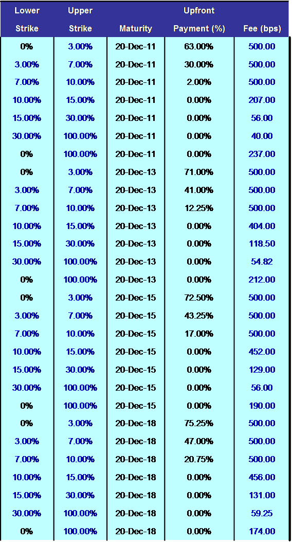
Figure 3: Tranche quotes for CDX.NA.IG11 on 04/15/09.

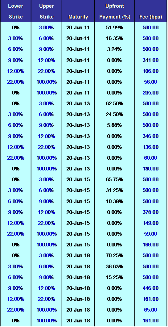
Figure 4: Tranche quotes for iTraxx Europe S9 on 04/15/09.

We calibrate the model to a set of tranche expected losses obtained using BSLP model of Ref.[2] (Results obtained using calibration to base correlation quotes will be reported below.). Calibration results are shown in Tables 1 and  2, where we display relative errors between the calculated and input tranche ELs obtained in the joint calibration of the model to CDX.NA.IG11 and iTraxx Europe S9 data. Note that as losses in senior tranches at short maturities are very small, large relative errors observed for these tranches give rise to very small pricing error in terms of tranche par spreads, thus rendering calibration nearly perfect. The implied distribution of the market factor is shown in Fig. 5.

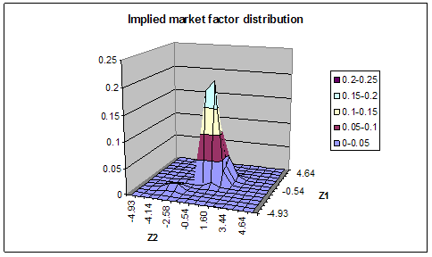
Figure 5: Implied distribution of the market factor on 04/15/09, calibration to CDX.NA.IG11 and iTraxx Europe S9.

Tranche	0-3%	3-7%	7-10%	10-15%	15-30%	$\Pi_{11}$	$\Pi_{12}$
1Y	-0.010	-0.067	71.313	-90.575	-81.617	0.016	-0.038
2Y	-0.005	-0.011	- 0.024	- 0.040	- 0.468	0.005	- 0.004
3Y	-0.000	- 0.002	0.000	0.003	0.003	0.000	-0.001
4Y	0.0059	0.002	0.0163	0.006	0.018	- 0.002	- 0.000
5Y	0.007	0.002	0.013	0.005	0.012	- 0.001	0.000

Table 1: Relative errors $\frac{EL_{model}-EL_{input}}{EL_{input}}$ (in percent) between input ELs for CDX.NA.IG11 and calculated model values obtained with joint calibration to CDX.NA.IG11 and iTraxx Europe 9 data on 04/15/2009.

Tranche	0-3%	3-6%	6-9%	9-12%	12-22%	$\Pi_{21}$	$\Pi_{22}$
1Y	-0.013	-0.033	-0.063	- 4.831	-25.914	0.021	-0.109
2Y	-0.001	0.008	-0.018	0.072	0.018	-0.000	- 8.039
3Y	0.001	0.006	0.006	-0.004	0.019	-0.001	- 2.403
4Y	0.001	0.004	0.010	0.000	0.017	- 0.001	- 0.572
5Y	0.001	0.002	0.007	0.006	0.012	- 0.001	- 0.106

Table 2: Relative errors $\frac{EL_{model}-EL_{input}}{EL_{input}}$ (in percent) between input ELs for iTraxx Europe 9 and calculated model values obtained with joint calibration to CDX.NA.IG11 and iTraxx Europe 9 data on 04/15/2009.

The result of pricing tranches referencing our bespoke portfolio are shown in Table 3 where strikes are chosen to coincide with standard strikes of the CDX.NA.IG portfolio. We show the results obtained with two sets of correlation parameters: for Case 1, we use $\rho=0.5$, $\alpha=0.3$, and for Case 2, we set $\rho=0.75$, $\alpha=0.0$. Note that inter-sector correlations are decreased in the second case by 10% relatively to the first one, see Eq.(12). Therefore, the effect of transition from Case 1 to Case 2 is as expected: junior spreads go up, while senior spreads go down. On the other hand, for both choices of correlation parameters we find that senior mezzanine and junior senior tranches are substantially more expensive in our model than in the Base correlation approach. We can also convert prices into equivalent base correlations, see Fig. 6.

Tranche		Base correlation			IMFM, case 1			IMFM, case 2
Low	Upper	Par	Risky	Default	Par	Risky	Default	Par	Risky	Default
strike	strike	spread	annuity	leg	spread	annuity	leg	spread	annuity	leg
0%	3 %	6000.9	1.435	0.861	6358.9	1.428	0.908	6623.1	1.382	0.915
3%	7%	2914.1	2.476	0.722	3035.5	2.543	0.772	3116.8	2.535	0.790
7%	10%	1655.8	3.325	0.551	2014.6	3.224	0.649	1991.1	3.247	0.647
10%	15%	893.6	3.948	0.353	1248.2	3.858	0.482	1229.6	3.835	0.472
15%	30%	329.65	4.507	0.149	409.2	4.524	0.185	403.4	4.538	0.183
30%	100%	130.15	4.407	0.057	63.4	4.786	0.030	63.6	4.785	0.031

Table 3: Pricing of tranches on the mixed CDX IG11-iTraxx9 bespoke portfolio with 5Y to maturity on 04/15/09. Case 1: $\rho=0.5$, $\alpha=0.3$. Case 2: $\rho=0.75$, $\alpha=0.0$.

Figure 6: Equivalent correlation skew for the mixed CDX IG11-iTraxx9 bespoke portfolio priced on 04/15/09.

To test the impact of different interpolation schemes used to calculate tranche expected losses on the time grid, we have performed comparison of results obtained with calibration of IMFM to tranche ELs obtained with the Base correlation (BC) model instead of ELs generated by BSLP. The results are shown in Table 4. It turns out that calibration to BC-generated tranche ELs produces larger pricing errors for short time maturities comparing to calibration to BSLP-generated ELs. The resulting bespoke tranche prices are however reasonably close to numbers obtained with the former method (we skip the results to save space).

Tranche		Base correlation			IMFM, case 1			IMFM, case 2
Low	Upper	Par	Risky	Default	Par	Risky	Default	Par	Risky	Default
strike	strike	spread	annuity	leg	spread	annuity	leg	spread	annuity	leg
0%	3 %	6000.9	1.435	0.861	7465.5	1.211	0.904	6623.1	1.382	0.915
3%	7%	2914.1	2.476	0.722	3407.8	2.271	0.774	3116.8	2.535	0.790
7%	10%	1655.8	3.325	0.551	2161.5	2.925	0.632	1991.1	3.247	0.647
10%	15%	893.6	3.948	0.353	1324.5	3.540	0.469	1229.6	3.835	0.472
15%	30%	329.65	4.507	0.149	433.3	4.435	0.192	403.4	4.538	0.183
30%	100%	130.15	4.407	0.057	67.3	4.766	0.032	63.6	4.785	0.031

Table 4: Pricing of tranches on the mixed CDX IG11-iTraxx9 bespoke portfolio with 5Y to maturity on 04/15/09. Case 1: calibration to ELs generated by Base correlation model. Case 2: calibration to ELs generated by BSLP model. For both cases, $\rho=0.75$ and $\alpha=0$.

Our second bespoke portfolio is a mixed portfolio of 125 US investment and non-investment grade names, priced on 05/15/09. It has 90 highest spread names from CDX.NA.IG11, while 35 lowest spread names from this index are substituted by 35 lowest spread names from CDX.NA.HY10 index. Market quotes on index tranches are shown in Figs. 7 and  8.

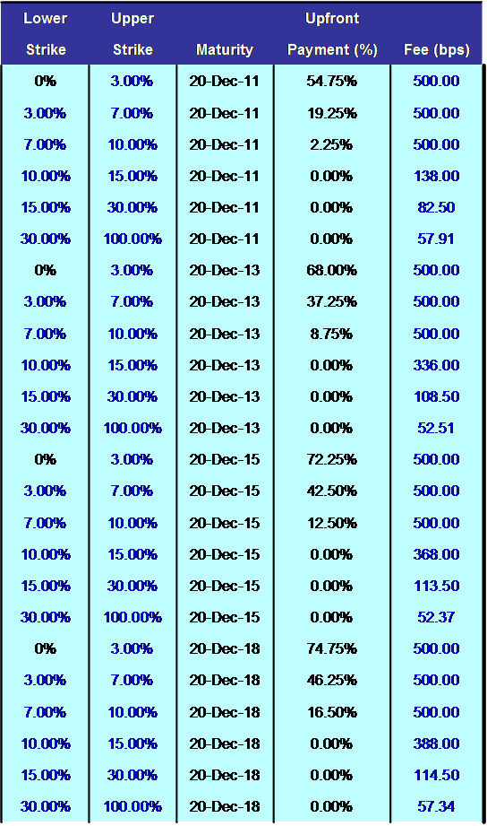
Figure 7: Tranche quotes for CDX.NA.IG11 on 05/15/09.

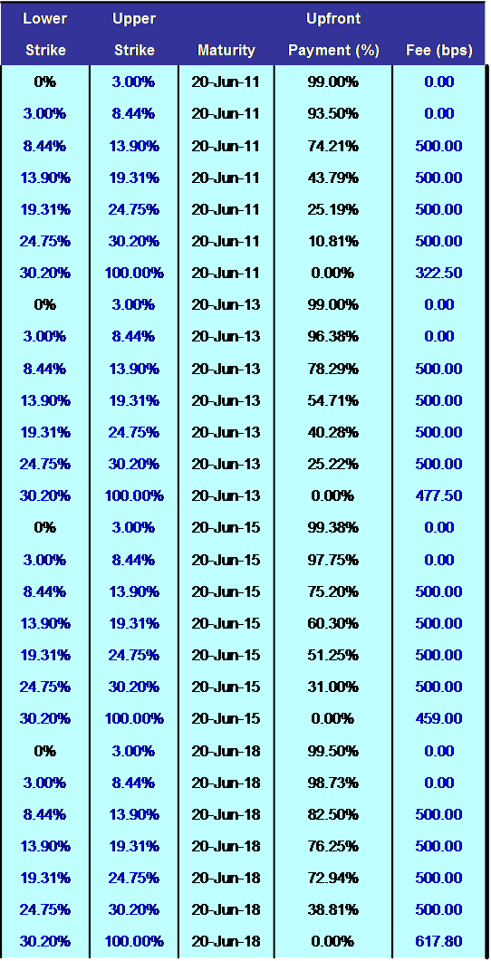
Figure 8: Tranche quotes for CDX.NA.HY10 on 05/15/09.

Calibration results are shown in Tables 5 and  6, where we display relative errors between the calculated and input tranche ELs obtained in the joint calibration of the model to CDX.NA.IG11 and CDX.NA.HY10 data. Similar to the above, large relative errors observed at short maturities do not have a material impact on the quality of calibration because losses in senior tranches at short maturities are very small anyway. The implied distribution of the market factor for this case is shown in Fig. 9. Unlike previous case, we now observe a pronounced bi-modal shape of the implied distribution.

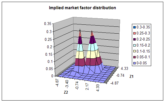
Figure 9: Implied distribution of the market factor on 05/15/09, calibration to CDX.NA.IG11 and CDX.NA.HY10.

Tranche	0-3%	3-7%	7-10%	10-15%	15-30%	$\Pi_{11}$	$\Pi_{12}$
1Y	-0.000	-0.005	-0.231	-93.745	-84.426	0.000	0.002
2Y	0.001	0.000	0.005	0.030	0.026	0.001	0.002
3Y	0.000	0.000	0.000	0.000	0.000	0.000	0.000
4Y	0.000	0.000	0.001	0.001	0.002	0.000	0.000
5Y	0.000	0.000	0.000	0.000	0.001	0.000	0.000

Table 5: Relative errors $\frac{EL_{model}-EL_{input}}{EL_{input}}$ (in percent) between input ELs for CDX.NA.IG11 and calculated model values obtained with joint calibration to CDX.NA.IG11 and CDX.NA.HY10 data on 05/15/2009.

Tranche	0-3%	3-8.4%	8.4-13.9%	13.9-19.3%	19.3-24.8%	24.8-30.2%	$\Pi_{21}$	$\Pi_{22}$
1Y	0.000	0.000	0.000	0.000	0.000	0.001	-0.001	0.000
2Y	0.000	0.000	0.000	0.000	0.000	0.000	0.000	0.000
3Y	0.001	0.001	0.001	0.001	0.001	0.007	0.001	- 1.315
4Y	0.000	0.000	0.000	0.000	0.000	0.001	0.000	- 5.115
5Y	0.000	0.000	0.000	0.000	0.000	0.001	0.000	- 5.264

Table 6: Relative errors $\frac{EL_{model}-EL_{input}}{EL_{input}}$ (in percent) between input ELs for CDX.NA.HY10 and calculated model values obtained with joint calibration to CDX.NA.IG11 and CDX.NA.HY10 data on 05/15/2009.

Results of pricing tranches on this portfolio with maturity of 5Y are shown in Table 7. Note that qualitatively the difference in resulting numbers between IMFM and BC is similar to results found for our previous example of a mixed CDX.IG-iTraxx bespoke portfolio, i.e. the largest discrepancy between the two models is obtained for senior mezzanine and junior senior tranches. Equivalent correlation skew in shown in Fig. 10.

Tranche		Base correlation			IMFM, case 1			IMFM, case 2
Low	Upper	Par	Risky	Default	Par	Risky	Default	Par	Risky	Default
strike	strike	spread	annuity	leg	spread	annuity	leg	spread	annuity	leg
0%	3 %	4554.1	1.81	0.821	3495.6	2.30	0.804	3503.9	2.29	0.804
3%	7%	2449.7	2.87	0.703	1633.7	3.48	0.569	1651.9	3.46	0.572
7%	10%	1224.1	3.79	0.464	1105.9	3.80	0.421	1121.7	3.77	0.423
10%	15%	738.8	4.25	0.314	1012.6	3.89	0.394	1020.1	3.90	0.398
15%	30%	275.1	4.60	0.127	438.3	4.49	0.197	439.2	4.49	0.197
30%	100%	72.8	4.54	0.033	53.7	4.79	0.026	52.3	4.79	0.025

Table 7: Pricing of tranches on the mixed CDX IG11-CDX HY10 bespoke portfolio with 5Y to maturity on 05/15/09. Case 1: $\rho=0.5$, $\alpha=0.3$. Case 2: $\rho=0.75$, $\alpha=0.0$.

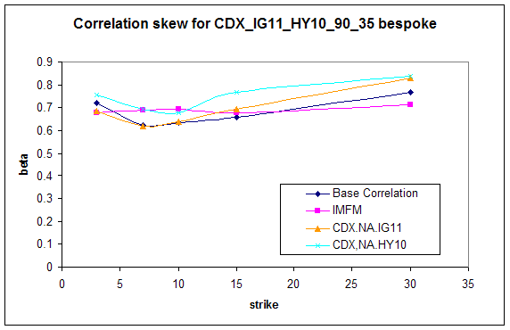
Figure 10: Equivalent correlation skew for the mixed CDX IG11-CDX HY10 bespoke portfolio priced on 05/15/09.

7 Conclusion

In this paper we have presented the Implied Multi-Factor model (IMFM) - a semi-parametric hybrid bottom-up/top-down model designed for pricing and risk management of tranches on bespoke portfolios, as well as other, more exotic derivatives referencing bespoke portfolios. The model ensures no-arbitrage in the bespoke pricing, and eliminates the need for ad hoc “base correlation mapping rules” that are often used by practitioners to price bespoke CDO tranches. The alternative suggested in this paper is to use instead standard tools of probability theory in combination with the Minimum Cross Entropy (MCE) method of statistical inference. The latter is employed to infer, an a least biased way, loss distributions of index portfolio implied by available prices of tranches referencing these portfolios.

Our framework differs from most of more traditional models in a number of points. First, our approach is semi-parametric, allowing one to automatically adjust the number of free parameters (and calibrate them) once the size of calibration set is changed. This produces a flexible and accurate calibration. In addition, this approach can be easily adjusted to accomodate e.g. quotes on sub-portfolios of index portfolios (or even tranches referencing bespoke portfolios) if traders are willing to provide such quotes. Second, the model is able to control the relative importance of fitting the data versus proximity to the “prior” model, thus providing means to avoid possible overfitting, or to find a solution in sutuations where constraints cannot be satisfied exactly. Third, calibration in our IMFM framework amounts to convex optimization in a low dimensional space. Therefore, the model is computationally efficient and calibrates within minutes rather than hours which we would expect for a more traditional bottom-up model with a multi-factor structure.

Last but not least, convexity of the calibration problem in our model leads to a unique solution. Recall that more traditional bottom-up approaches to modeling credit portfolios typically give rise to objective functions having multiple local minima. When the model is re-calibrated from one day to another, the presence of local minima poses a problem, as a local search algorithm typically used for calibration might end up in a different local minimum from that found a day earlier, leading to unstable calibration and hedge ratios. Our model is free of such potential pitfalls.

We have formulated two versions of the model. The first, single-period (“static”) version can be used for pricing bespoke CDO tranches. The second, dynamic version of the model can be used to price and risk-manage other, more exotic portfolio derivatives, such as e.g. forward-starting tranches or tranche options. Another potential application for the dynamic version of our model is the counterparty risk management (including, in particular, CVA calculations) for CDO tranches. Because the model is low-dimensional and Markovian, efficient lattice or tree implementations are possible.

The approach presented in this paper is readily generalizable and extensible. Even though we presented details and numerical examples only for the basic case involving two market factors and two reference index portfolios for a given bespoke portfolio, we have shown how to generalize this setting to more complex cases including more reference portfolio, more market factors, and handling names not belonging in any index portfolio. Further extensions including risk management of bespoke tranches and modeling of price uncertainty of bespoke tranches due to bid/ask spreads of index tranches will be presented elsewhere.

Appendix: Mutual information and portfolio loss partitioning

As was mentioned above, the solution (3.2) indicates that the conditional independence of losses in sub-portfolios does not hold for the “posterior” model that adjust the “prior” distributions so that pricing constraints referencing portfolios as a whole are respected. In this section, we discuss this phenomenon in more details.

We start with an intuitive explanation. Assume we have two subportfolios $\Pi_{11}$ and $\Pi_{12}$ of an index portfolio $\Pi_{1}$. whose losses $X\equiv X_{11}$ and $Y\equiv X_{12}$ are assumed to be independent a priori. Obviously, if we know the loss $L$ in the whole portfolio with certainty, $L=L_{0}$, then instead of independence of $X$ and $Y$ we have a deterministic dependence between them as now $Y=L_{0}-X$. By continuity, we should expect that when instead of knowing losses with certainty we only know the expectation of $L$ (as $L$ should generally be treated as a random variable), we should expect a probabilistic dependence between $X$ and $Y$, because the previous deterministic case would be recovered in the limit when the loss distribution is a delta function centered at $L_{0}$: $\langle L\rangle\equiv\int dL\,Lp(L)\rightarrow\int dL\,L\delta(L-L_{0})=L_{0}$. This implies that the more information (less uncertainty) we have about the distribution of $L$, the more informative $X$ and $Y$ should be about each other.

Let us make this intuitive argument a bit more formal. A model-free information-theoretic measure of dependence between two random variables $X$ and $Y$ is the mutual information

$$I(X;Y) = \mathbb{E}_{p(x,y)}\left[\log\frac{p(X,Y)}{p(X)p(Y)}\right]=\int dxdy\,p(x,y)\log\frac{p(x,y)}{p(x)p(y)}=\int dxdy\,p(x)p(y|x)\log\frac{p(y|x)}{p(y)}$$ (B.1)

$$= \int dxdy\,p(x)p(y|x)\log\frac{p(y|x)}{\int p(x^{\prime})p(y|x^{\prime})dx^{\prime}}$$

In particular, it follows by Jensen’s inequality that $I(X;Y)\geq 0$, while the equality is reached iff the two variables are independent, i.e. $p(x,y)=p(x)p(y)$, see e.g. [6]. It is easy to check that unconstrained minimization of (B.1) with respect to $p(y|x)$ yields a factorized solution. Indeed, the variational derivative of (B.1) reads

$$\frac{\delta I}{\delta p(y|x)}=p(x)\log\frac{p(y|x)}{p(y)}=p(x)\log\frac{p(x,y)}{p(x)p(y)}$$ (B.2)

which vanishes when $p(y|x)=p(y)$ or equivalently $p(x,y)=p(x)p(y)$.

Let us now assume we are given constraints in the form of expectations $\langle F_{i}(x+y)\rangle_{p(x,y)}=C_{i}$. The minimum mutual information consistent with these constraints should be found by minimization of the following Lagrangian

$$\mathcal{L}=I(X;Y)-\sum_{i}\lambda_{i}\left(\int dxdy\,p(x)p(y|x)F_{i}(x+y)-C_{i}\right)-\int dx\,\xi(x)\left(\int dy\,p(y|x)-1\right)$$ (B.3)

where $\lambda_{i}$ and $\xi(x)$ are Lagrange multipliers. This variational problem has the formal solution

$$p(y|x)=p(y)e^{\sum_{i}\lambda_{i}F_{i}(x+y)+\xi(x)}$$ (B.4)

While this solution is only a formal one as $p(y)$ in turn depends on $p(y|x)$ by the marginalization condition $p(y)=\int dx\,p(x)p(y|x)$, it clearly shows that unless all $\lambda_{i}=0$, the conditional probability $p(y|x)$ does depend on $x$ (as long as functions $F_{i}(x)$ are non-linear), i.e. the independence solution $p(x,y)=p(x)p(y)$ cannot hold anymore. Physically, this means that the knowledge of expectations of functions of the form $F_{i}(X+Y)$ carries information on interaction between two sub-portfolios (i.e. has a non-vanishing information value), and is in general incompatible with the independence assumption.

In our setting involving the market factor $Z=\vec{Z}_{\vec{m}}$ described by a set of discretized probabilities $\{h_{\vec{m}}\}$, another relevant object is the conditional mutual information of sub-portfolio losses $X\equiv X_{11}$ and $Y=X_{21}$ given $Z_{\vec{m}}$:

$$I(X;Y|Z) = \mathbb{E}_{p(x,y,z)}\left[\log\frac{p(X,Y|Z)}{p(X|Z)p(Y|Z)}\right]=\sum_{\vec{m}}h_{\vec{m}}\int dxdy\,P\left(x,y|\vec{m}\right)\log\frac{P(x,y|\vec{m})}{P_{X}(x|\vec{m})P_{Y}(y|\vec{m})}$$ (B.5)

$$= \sum_{\vec{m}}h_{\vec{m}}\int dxdy\,P_{X}(x|\vec{m})P_{Y}(y|x,\vec{m})\log\frac{P_{Y}(y|x,\vec{m})}{\int P_{X}(x^{\prime}|\vec{m})P_{Y}(y|x^{\prime},\vec{m})dx^{\prime}}$$

The same calculation with (B.5) results in factorization of conditional probabilities $P(x,y|\vec{m})=P_{X}(x|\vec{m})P_{Y}(y|\vec{m})$, i.e. in conditional independence.

Coming back to the unconstrained case, let us continue with the example of two random variables $X$ and $Y$ discussed above, which will now be identified with losses in sub-portfolios $\Pi_{X}$ and $\Pi_{Y}$, respectively. We assume that $X$ and $Y$ are independent a priori, which is the case when we condition on the market factor $Z$. As we have seen above, unconstrained minimization of mutual information (MI) $I(X;Y)$ yields the factorization (independence) result $p(x,y)=p(x)p(y)$, but what should we take for marginal distributions $p(x)$ and $p(y)$? Clearly, if we have some initial guesses (e.g. obtained with historical calibration) $q(x)$ and $q(y)$ for the marginals, it is natural to expect that in the absence of any constraints we should have $p(x)=q(x)$, $p(y)=q(y)$ and $p(x,y)=p(x)p(y)=q(x)q(y)$. Formally, we can achieve this by minimization of the following functional

$$\mathcal{F}[p(x),p(y|x)]=I(X;Y)+D[p(y)||q(y)]+D[p(x)||q(x)]$$ (B.6)

where $D[p||q]$ is the KL distance between two distributions $p$ and $q$. Indeed, as all terms here are non-negative, the whole expression is minimized when each term vanishes, which happens exactly for the case $p(x)=q(x)$, $p(y)=q(y)$ and $p(x,y)=p(x)p(y)=q(x)q(y)$. We can now combine the first two terms in (B.6) to get a more explicit expression

$$\mathcal{F}[p(x),p(y|x)]=\int dxdy\,p(x)p(y|x)\log\frac{p(y|x)}{q(y)}+\int dx\,p(x)\log\frac{p(x)}{q(x)}=D[p(x,y)||q(x)q(y)]$$ (B.7)

In other words, we ended up with the objective function which is nothing but the KL distance between the unknown distribution $p(x)$ and a factorized “prior” distribution $q(x,y)=q(x)q(y)$. This provides a justification to the method used in the main text, where we mimimize KL distances between conditional joint loss distributions of sub-portfolios and prior joint distributions, conditional on pricing constraints that reference portfolios as a whole.

Information has been obtained from sources believed to be reliable but JPMorgan Chase & Co. or its affiliates and/or subsidiaries (collectively JPMorgan) does not warrant its completeness or accuracy. Opinions and estimates constitute our judgement as of the date of this material and are subject to change without notice. Past performance is not indicative of future results. This material is not intended as an offer or solicitation for the purchase or sale of any financial instrument. Securities, financial instruments or strategies mentioned herein may not be suitable for all investors. The opinions and recommendations herein do not take into account individual client circumstances, objectives, or needs and are not intended as recommendations of particular securities, financial instruments or strategies to particular clients. The recipient of this presentation must make its own independent decisions regarding any securities or financial instruments mentioned herein. JPMorgan may act as market maker or trade on a principal basis, or have undertaken or may undertake account transactions in the financial instruments or related instruments of any issuer discussed herein and may act as underwriter, placement agent, advisor or lender to such issuer. JPMorgan and/or its employees may hold a position in any securities or financial instruments mentioned herein. Important disclosures are available on a company specific basis at http://mm.jpmorgan.com/disclosures/company. Additional information available upon request.

References

- [1] A. Anderson and J. Sidenius, “Extensions to the Gaussian Copula: Random Recovery and Random Factor Loadings”, Journal of Credit Risk, 1 (2004) 29.
- [2] M. Arnsdorf and I. Halperin, ”BSLP: Bivariate Spread-Loss Model for Portfolio Credit Derivatives”, Journal of Computational Finance 12 (2008) 77.
- [3] M. Avellaneda, R. Holmes. C. Friedman and D. Samperi, “Calibration of Volatility Surfaces via Relative-Entropy Minimization”, Applied Mathematical Finance”, March 1997, 4; M. Avellaneda, “Minimum Relative Entropy Calibration of Asset-Pricing Models”, International Journal of Theoretical and Applied Finance 1 (1998), 447.
- [4] P.W. Buchen and M.F. Kelly, “The Maximum Entropy Distribution of an Asset Inferred from Option Prices”, Journal of Financial and Quantitative Analysis, 31 (1996) 143.
- [5] A. Chapovsky, A. Rennie, and P.A.C. Tavares, “Stochastic Intensity Modelling for Structured Credit Exotics”, working paper (2006), available at www.defaultrisk.com.
- [6] T.M. Cover and J. A. Thomas, Elements of Information Theory, Wiley, second edition, 2006.
- [7] D. Duffie and Garleanu, “Risk and Valuation of Collateralized Debt Obligations”, Financial Analyst Journal, 57 (2001) 41.
- [8] K. Giesecke and L. Goldberg, “A Top Down Approach to Multi-Name Credit” (2005), available on www.defaultrisk.com.
- [9] A. Globerson and N. Tishby, “ The Minimum Information Principle for Discriminative Learning”, in C. Meek and J. Halpern, eds, Proceedings of the 20th Annual Conference on Uncertainty in Artificial Intellegence (UAI-04), (2004).
- [10] L. Gulko, “The Entropy Theory of Option Pricing” Yale University Working Paper (1995); “The Entropy Pricing Theory”, Ph.D. Thesis, Yale School of Management (1998).
- [11] I. Halperin, “Bayesian Entropic Inverse Theory Approach to Implied Option Pricing with Noisy Data”, available at http://xxx.lanl.gov/abs/cond-mat/0209146.
- [12] I. Halperin, “Random Thinning of Credit Portfolio Dynamics and Predictive Filtering”, JPM (2006).
- [13] I. Halperin, “Pricing of Index and Bespoke CDO Tranches with Minimum Cross Entropy”, presentation at Credit Risk Summit, NYC October 2006.
- [14] I. Halperin and P. Tomecek, ”Climbing Down from the Top: Single-Name Dynamics in Top-Down Credit Models”, working paper, JPM (2008).
- [15] J. Hull and A. White, ”Valuing Credit Derivatives Using an Implied Copula Approach to”, Journal of Derivatives 12 (2) (2006) 8.
- [16] J. Hull and A. White, ”An Improved Implied Copula Model and its Application to the Valuation of Bespoke CDO Tranches”, working paper (2008).
- [17] Inglis and A. Lipton, “Factor Models for Credit Correlation”, working paper (2007); RISK 22 (2009) 98.
- [18] D. Li, “On Default Correlation: A Copula Approach”, Journal of Fixed Income 9 (2000), 43.
- [19] D. O’Kane, Modelling Single-Name and Multi-Name Credit Derivatives, Wiley (2008).
- [20] D. Rosen and D. Saunders, ”Valuing CDOs of Bespoke Portfolios with Implied Multi-Factor Models”, working paper (2008).
- [21] P. Schönbucher, “Portfolio Losses and the Term Structure of Loss Transition Rates”, working paper (2005).
- [22] J. Sidenius, V. Piterbarg, and L. Andersen, “A New Framework for Dynamic Credit Portfolio Modelling”, working paper (2005).
- [23] M. Stutzer, “A Simple Nonparametric Approach to Derivative Security Valuation”, Journal of Finance, 51 (1996) 1633.
- [24] G. Turc et al, “ Pricing Bespoke CDOs: latest developments”, Societe Generale (2006).
- [25] A. Veremeyev, A. Nakonechnyi, S. Uryasev and R.T. Rockefellar, “Implied Copula CDO Pricing Model: Entropy Approach”, working paper (2009).
- [26] L. Vacca, “Market-Implied Archimedian Copulas”, RISK, January 2008, 104.
- [27] R. Zhou, ”A Multi-Portfolio Model for Bespoke CDO Pricing, Part I: Methodology ”, working paper (2008).