The glass transition of two-dimensional binary soft disk mixtures with large size ratios

Abstract

We simulate binary soft disk systems in two dimensions, and investigate how the dynamics slow as the area fraction is increased toward the glass transition. The “fragility” quantifies how sensitively the relaxation time scale depends on the area fraction, and the fragility strongly depends on the composition of the mixture. We confirm prior results for mixtures of particles with similar sizes, where the ability to form small crystalline regions correlates with fragility. However, for mixtures with particle size ratios above 1.4, we find that the fragility is not correlated with structural ordering, but rather with the spatial distribution of large particles. The large particles have slower motion than the small particles, and act as confining “walls” which slow the motion of nearby small particles. The rearrangement of these confining structures governs the lifetime of dynamical heterogeneity, that is, how long local regions exhibit anomalously fast or slow behavior. The strength of the confinement effect is correlated with the fragility and also influences the aging behavior of glassy systems.

I Introduction

Many liquids can form glasses if they are cooled rapidly, and glassy materials have technological applications such as optical fibers and plastics Debenedetti ; Angell ; Angell2 ; Ediger ; Kob . The origin of the glass transition is still unclear, despite the scientific and technological interests. Much work has examined the dynamical properties of materials near the glass transition. Those studies revealed several important features of supercooled liquids and glasses. For example, upon approaching the glass transition, the structural relaxation time ($\tau_{\alpha}$) increases by several orders of magnitude without a corresponding growing static correlation length ernst91 ; vanblaaderen95 . The rate of this increase of $\tau_{\alpha}$ is called “fragility” and depends on the material Debenedetti ; Angell ; Angell2 ; Ediger ; Kob . For fragile glass-formers, $\tau_{\alpha}$ steeply increases for a small decrease in temperature, while for “strong” glass-formers, the increase of $\tau_{\alpha}$ requires a larger decrease in temperature. The relaxation time is related to the viscosity, and thus the fragility is an important factor in the ease of processing glass-forming materials. Typically it is desirable to mold a glass-forming material with the viscosity held within a certain range; for fragile materials, this may correspond to a restrictively narrow range of temperature.

Another common observation of materials close to the glass transition is that they often have a broad distribution of local mobility: some regions in a sample relax much faster than other regions. Eventually, molecules in those regions exchange their dynamics, that is, fast regions become slow and vice versa. This is termed “dynamical heterogeneity” kob97 ; donati98 ; Ediger2 ; Harrowell ; Eric1 ; Berthier ; Yamamoto . It is known that the characteristic lifetime of these dynamically heterogeneous regions $\tau_{DH}$ is longer than $\tau_{\alpha}$ and the strong divergence of $\tau_{DH}$ near a glass transition temperature suggests that heterogeneous dynamics are relevant for understanding the glass transition Ediger .

A third common feature of materials in the glassy state is that their properties evolve with time, such as the diffusivity of molecules or dielectric susceptibility. This phenomenon is termed “aging” Angell3 ; Hodge ; Megen ; courtland03 ; Gianguido ; Jenn . Despite the changing properties, no clear structural changes have been seen; this can be true even if, for example, diffusivity slows by several orders of magnitude Gianguido ; Jenn .

While all of these properties have been known for some time and carefully characterized by experiments, the origins of many of them are unclear. To understand the origins, numerical simulations with simple intermolecular interactions are used to study factors controlling the dynamics. These model systems are useful as clear understanding is hindered by the complexity of real materials Onuki ; KAT ; Sun ; Coslovich ; Tarjus . For the fragility, some simulations show that liquids become less fragile when the polydispersity increases (or a larger size ratio for binary mixtures is used) KAT ; Sun ; Coslovich . This has been explained as due to ordering of the sample, which becomes frustrated in polydisperse samples. For example, in two-dimensional (2D) systems, small regions with hexagonal order can form which correspond with slower dynamics (larger values of $\tau_{\alpha}$), and thus increasing the polydispersity frustrates formation of these ordered regions and diminishes the fragility KAT . Furthermore, it is reported that particle mobility in those ordered regions are slower than that in randomly structured regions and it suggests that dynamical heterogeneity is also influenced by local structure KAT ; Tarjus ; weeks02 ; harrowell04 ; widmercooper05 ; widmercooper08 ; conrad05 ; matharoo06 ; berthier07 ; appignanesi09 .

Those simulations used the polydispersity as a small perturbation frustrating the ordering, that is, with either a small polydispersity or a binary system with the particle size ratio close to 1. However, dynamics in those situations are quite different from highly polydisperse samples. Binary mixtures have two control parameters: the size ratio and the volume fraction ratio of the two components. These lead to complex phase diagrams Imhof ; dinsmore95 and potentially emergent dynamical properties such as an effective depletion interaction between the large particles in binary hard sphere systems AO ; crocker99 . Our interest is in dense amorphous phases at intermediate size ratios.

In this article, we simulate the dynamics of binary soft disk mixture systems with large size ratios and find that the glass transition in large size ratio binary systems can be quite different from that of systems with smaller size differences. We study the fragility of binary soft disk mixtures with various size ratios and area fraction ratios. Local ordering is less significant for large size ratio systems. Instead, we see a molecular crowding effect from the large particles moreno06 ; voigtmann09 . Our data suggest that the large particles act as confining walls for the smaller particles, and that confinement effects increase the fragility of such systems by suppressing dynamical heterogeneity. We also investigate aging in large size ratio systems, and again seen an influence of confinement effects due to the large particles. Overall, our results suggest that confinement effects are crucial to describing the dynamics of the glass transition in binary mixtures with large size ratios between the two components.

II Method

We perform two-dimensional Brownian dynamics simulations for binary mixtures composed of large ($L$) and small ($S$) soft particles. These simulations are meant to mimic the colloidal glass transition. For the colloidal glass transition, the key control parameter is the volume fraction vanblaaderen95 ; Eric1 ; pusey86 , and so in our simulations the chief control parameter is the area fraction $\phi$. The results of Brownian Dynamics simulations are similar to those of molecular dynamics simulations in dense systems KAT ; Coslovich ; gleim98 ; szamel04 ; tokuyama07 . The particles interact via the purely repulsive Weeks-Chandler-Andersen potential WCA ; $U_{ij}=4\epsilon[(\sigma_{ij}/r)^{12}-(\sigma_{ij}/r)^{6}+1/4]$ for $r<2^{1/6}\sigma_{ij}$, otherwise $U_{ij}=0$, where $\sigma_{ij}=(\sigma_{i}+\sigma_{j})/2$ and $i,j\in\{L,S\}$. We fix $k_{B}T/\epsilon=0.04$, so the total area fraction $\phi$ is our control parameter to approach the glass transition. The mass ratio is $m_{L}/m_{S}$=$(\sigma_{L}/\sigma_{S})^{2}$ and the length is normalized by $\sigma_{S}$. The total number of particles is $N=N_{L}+N_{S}=1024$ (or 4096) where $N_{L}$ and $N_{S}$ are the number of large and small species, respectively. We generate initial conditions by simulating at $\phi=0.10$ for a long time and expanding the disk sizes to increase $\phi$. We confirm that our results do not show initial condition dependence and our results are also independent on time below $\phi=0.66$, that is, there is no aging observed. Thus, we consider our binary systems are well mixed and ergodic for $\phi<0.66$.

For certain area fractions for a 2D monodisperse sample, the hexatic order phase can be found, which has orientational order but no long-range positional order Halperin . For binary samples with large size ratios, there is apparently little ordering of either type, while for size ratios close to 1, hexatic phases are still subtle to verify. Hence, we calculate an orientation pair correlation function $g_{6}(R)/g(R)$ where $R$ is a normalized distance from a particle. $g_{6}(R)/g(R)$ decays with the power of $R^{-1/4}$ in a hexatic phase for a monodisperse sample Halperin . Thus, we classify our samples as liquid (or glassy) when the power of the decay is faster than $R^{-1/4}$ [Fig. 1]. We find no hexatic phases for any area fractions $\phi$ for systems with size ratios $\sigma_{L}/\sigma_{S}$=1.2, 1.25, 1.5, 1.75, 2, 2.5 and 3 and area fraction ratios $\phi_{L}/\phi_{S}$=$N_{L}\sigma_{L}^{2}/N_{S}\sigma_{S}^{2}$=0.5, 0.75, 1, 1.5 and 2; these states are indicated by the circles in Fig. 2(a). We confirm that the decay rates of $g_{6}(R)/g(R)$ in those simulation conditions are quicker than $R^{1/4}$ and thus we are studying liquids (or glasses at higher $\phi$). We note that it is known that several crystalline structures exist in three-dimensional (3D) binary sphere suspensions Imhof ; kikuchi07 . In none of our samples do we observe large hexagonally ordered patches for our simulations, and the small patches that sometimes appear are transient. This is discussed further below.

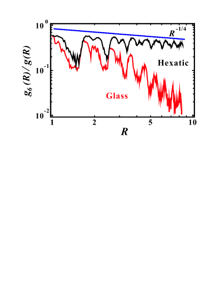
Figure 1: (Color online.) The orientation pair correlation as a function of distance. The straight line corresponds to $R^{-1/4}$, the behavior expected for hexatic phases. A sample with size ratio $\sigma_{L}/\sigma_{S}$=1.2 and area fraction ratio $\phi_{L}/\phi_{S}$ = 0.5 at $\phi$ = 0.66 does not have hexatic order since $g_{6}(R)/g(R)$ decays faster than the power of $-1/4$ (the lower curve, marked “Glass”). In contrast, the upper curve (marked “Hexatic”) shows the correlation for $\sigma_{L}/\sigma_{S}$=1.15, $\phi_{L}/\phi_{S}$ = 0.5, and $\phi$ = 0.66, which has long range orientational ordering.

When the size ratio is large, a depletion force should be generated AO . This has been studied before in dilute suspensions of large and small spheres, and manifests itself as an effective attractive force between the large spheres crocker99 . We cannot rule out the existence of the depletion force in our simulations, which may affect the structure of the large particles, although at large area fractions the depletion force may be less relevant. Indeed, we observe pairs of adjacent large particles which neighbors for long periods of time, but these neighbors separate eventually (see Movie S1, EPAPS materials to be submitted), and in general all of the dynamics are slow in our glassy experiments. It’s unclear if depletion introduces still slower dynamics, or if this is merely part of the overall slow behavior. At least, we note that our systems are quite different from gels with strong attractive force.

III Results

III.1 Fragility: behavior as $\phi$ increases

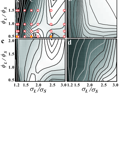
Figure 2: (color online). The contour plot of (a) fragility index $D$, (b) the growth rate of hexagonal order $\partial\langle\psi_{6}\rangle/\partial\phi$, (c) the growth rate of dynamical correlation length $\partial\xi/\partial\phi$ and (d) the dynamical correlation around a large particle $\Theta$ in a plane of ($\sigma_{L}/\sigma_{S}$, $\phi_{L}/\phi_{S}$). All those figures except (a) are obtained at $\phi$=0.66. The shading in each figure is darker when each value is small, thus, the darker regions correspond to (a) fragile liquids, (b) low growth of hexagonal order, (c) low growth of dynamical correlation length and (d) minimal correlations of motion between a large particle and its neighbors. The circles in (a) are the simulated points and the specific states A, B, C, D, E and F are labeled.

We obtain the relaxation time $\tau_{\alpha}$ from the self-part of the intermediate scattering function for all particles, which is given by $F(k,t)$=$\frac{1}{N}\sum_{j}\langle\exp{i\vec{k}\cdot[\vec{r}_{j}(t)-\vec{r}_{j}(0)]}\rangle,$ where $\vec{r}_{j}$ is the position vector of particle $j$, $\langle\rangle$ indicates a time average and $\vec{k}$ is the wave vector. $\tau_{\alpha}$ is determined when $F(k_{p},\tau_{\alpha})$=$1/e$ where $k_{p}$ corresponds to the wave number of the first peak of the structure factor. The $\phi$ dependence of $\tau_{\alpha}$ is well fitted by Vogel-Fulcher function substituting $\phi$ for $1/T$: $\tau_{\alpha}$=$\tau_{0}\exp[D\phi/(\phi_{0}-\phi)]$, where $D$ is the fragility index and $\phi_{0}$ is the area fraction of the ideal glass transition [see Fig. 3(a)] Angell2 . Fragile liquids have smaller values of $D$. For example, $D\sim 4$ for triphenyl phosphite which is one of the most fragile liquids, while for the less fragile liquid butyronitrile, $D\sim 30$ Bohmer2 . For our simulations, $0.4\lesssim D\lesssim 1.0$, smaller than the molecular liquids. The difference may be due to using the density as the control parameter rather than temperature. For comparison, we examined the data of Refs. brambilla09 ; elmasri09 which used light scattering to study the colloidal glass transition as a function of volume fraction. From their data, we find $D=0.497\pm 0.002$. Another example is that the fragility index of glycerol in an isothermal experiment is smaller than that measured in an isobaric experiment Cook . We expect our observed qualitative dependence of the fragility on the system parameters to still be revealing.

It is worth noting that for our data, we also compute the value of $D$ by calculating $F(k,t)$ for only small particles (or large particles) and we obtain almost the same values for $D$ and $\phi_{0}$. We do not see separate glass transitions for the two particle species, which has been seen in simulations with large size ratios and equal particle numbers (thus volume fraction ratios $\phi_{L}/\phi_{S}$ much larger than ours) moreno06 ; voigtmann09 . In such cases, the large particles do not seem to interact as directly with the small particles but rather have their own glass transition, and then the small particles move in the interstices between the large particles. In our simulations, the volume fraction ratios are somewhat close to 1, and so the large particles always “see” the small particles and the alpha relaxation time scales for both particle species have similar $\phi$ dependence.

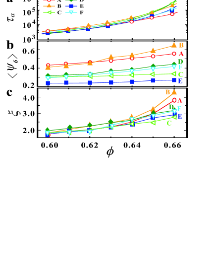
Figure 3: (Color online.) The area fraction $\phi$ dependence of (a) the relaxation time $\tau_{\alpha}$, (b) average hexagonal ordering $\langle\psi_{6}\rangle$ and (c) the dynamic correlation length $\xi$ at states A, B, C, D, E and F indicated in Fig. 2(a). The solid lines in (a) are fitting lines with the Vogel-Fulcher function at each state. Filled and open symbols correspond to fragile liquids and less fragile liquids, respectively.

Figure 2(a) shows the contour plot of the fragility $D$ in a ($\sigma_{L}/\sigma_{S}$, $\phi_{L}/\phi_{S}$) plane. The circles indicate the states simulated. This figure shows that the fragility is a non-monotonic function of the size ratio or the area fraction ratio. For example, for $\phi_{L}/\phi_{S}=2.0$, the fragility has values $D=1.05,0.82,0.45$ for states A, C, and E, but then increases slightly to 0.49 for the state to the right of E. Likewise, for $\phi_{L}/\phi_{S}=0.5$, the fragility behaves non-monotonically with increasing size ratio: $D=0.64,0.48,0.77$ for states B, D, and F. Comparing states A and B, or C and D, suggests that increasing the number of large particles increases the fragility index $D$, but states E and F disprove this trend.

We find that fragile liquids (small $D$) have small $\phi_{0}$, the area fraction where $\tau_{\alpha}$ appears to diverge. The relationship between fragility and the divergence point of $\tau_{\alpha}$ is observed at glass-forming liquids Tanaka ; KT2 and our results are consistent with them. On the other hand, the existence of $\phi_{0}$ for molecular liquids is still discussed and not well established Nm ; Phi0 . We are not sure what determines $\phi_{0}$ and why fragility is related to the divergence point. Below, we focus on microscopic properties such as particle mobility and local arrangement.

Prior work observed that two-dimensional systems can form small hexagonally ordered regions, and the mobility of particles is diminished within these regions. More fragile liquids are observed to have large growth rates of the size of these regions with respect to $\phi$ KAT ; Sun ; Coslovich . To check this we study the $\phi$ dependence of hexagonal order for our samples. We use the local hexatic order parameter described as $\psi_{6}^{j}=\frac{1}{n_{j}}\mid\sum^{n_{j}}_{m=1}e^{i6\theta_{m}^{j}}\mid$ where $n_{j}$ is the number of nearest neighbors for particle $j$ and $\theta_{m}^{j}$ is the angle of the relative vector $\vec{r}_{m}-\vec{r}_{j}$ with respect to the $x$ axis. $\psi_{6}^{j}$=1 means that a hexagonal arrangement is formed around particle $j$, while $\psi_{6}^{j}$=0 corresponds to a non-hexagonal arrangement. We then consider $\langle\psi_{6}\rangle$, the time and particle average of $\psi_{6}^{j}$. We compare the $\phi$ dependence of $\langle\psi_{6}\rangle$ with that of $\tau_{\alpha}$ [Fig. 3(a) and (b)]. Both particle sizes are similar at states A and B, $\sigma_{L}/\sigma_{S}=1.2$, and here both $\tau_{\alpha}$ and $\langle\psi_{6}\rangle$ increase dramatically as $\phi$ increases, suggesting they are indeed related as seen in prior work. However, for states C and E, $\langle\psi_{6}\rangle$ stays nearly constant with increasing $\phi$, while $\tau_{\alpha}$ grows rapidly. The system slows without significant hexagonal ordering.

Next, we compare the fragility with the growth rate of hexagonal ordering $\partial\langle\psi_{6}\rangle/\partial\phi$ since fragility corresponds to $\partial\log\tau_{\alpha}/\partial\phi$. (We calculate all derivatives of a quantity $X$ with respect to $\phi$ as $\partial X/\partial\phi=[X(\phi)-X(\phi-\Delta\phi)]/\Delta\phi$ where we choose $\Delta\phi=0.01$. In the results below, we compare the behavior of the samples at a fixed $\phi=0.66$. However, our results show similar trends when compare samples at fixed $\tau_{\alpha}$.) Figure 2(b) shows the contour plot of $\partial\langle\psi_{6}\rangle/\partial\phi$ at $\phi=0.66$ in a plane of ($\sigma_{L}/\sigma_{S}$, $\phi_{L}/\phi_{S}$). The growth of hexagonal order is small at large $\sigma_{L}/\sigma_{S}$ and $\phi_{L}/\phi_{S}$ (upper right region). This behavior is expected since hexagonal ordering should be frustrated with increasing $\sigma_{L}/\sigma_{S}$. Figure 4(a) shows $D$ as a function of $\partial\langle\psi_{6}\rangle/\partial\phi$. We observe two distinct behaviors. For similar particle size systems ($\sigma_{L}/\sigma_{S}<1.4$, triangles), more fragile liquids (smaller $D$) have a larger dependence of hexagonal order on $\phi$, in agreement with prior work KAT . In contrast, large size ratio systems ($\sigma_{L}/\sigma_{S}>1.4$, circles) show less correlation between the growth of hexagonal order and the fragility index.

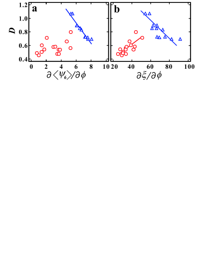
Figure 4: (Color online.) The fragility index $D$ as a function of (a) $\partial\langle\psi_{6}\rangle/\partial\phi$ and (b) $\partial\xi/\partial\phi$ at $\phi$=0.66. The triangles correspond to systems where size ratio is close to 1 ($\sigma_{L}/\sigma_{S}<1.4$) and the circles correspond to large size ratios ($>1.4$). The lines are added as guides to the eye.

Cooperative motion of groups of particles is a common phenomenon as the glass transition is approached Ediger2 ; Eric1 ; Harrowell ; Berthier ; Doliwa ; Eric2 , and this behavior is thought to be more common in fragile glasses. Figure 5(a) and (c) show snapshots of the systems at $\phi$ = 0.66 at state B and state E, where particles are colored based on $\Delta r_{j}^{2}$, and groups of highly mobile particles are seen (darker colors). To define displacements, here (and for the subsequent analysis in this work) we focus on the time scale $\Delta t^{*}$ for which the non-Gaussian parameter is the largest. The non-Gaussian parameter is defined as

$$\alpha_{2}(\Delta t)=\frac{3\langle\Delta r^{4}\rangle}{5\langle\Delta r^{2}\rangle^{2}}-1$$ (1)

with displacements $\Delta r$ measured over the lag time $\Delta t$, and the factor of 3/5 chosen so that $\alpha_{2}=0$ for a Gaussian distribution rahman64 . $\alpha_{2}$ is larger when the tails of the distribution become broad. Prior work identified the time scale $\Delta t^{*}$ that maximizes $\alpha_{2}$ as related to cage rearrangements kob97 ; donati98 ; Eric1 . In our current work, we computed $\alpha_{2}$ separately for the large and small particles, finding similar values for $\Delta t^{*}$. For our analysis, we will use $\Delta t^{*}$ based on $\alpha_{2}$ calculated for the small particles, and our results are not sensitive to this choice.

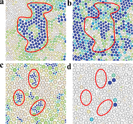
Figure 5: (Color online.) (a) and (b) are snapshots of the system at state B, $\phi=0.66$; (c) and (d) are at state E, $\phi=0.66$. The simulation box is four times as large as those snapshots in each side. In (a) and (c), particles are colored based on mobility $\Delta r_{j}^{2}$, with darker colors indicating more mobile particles. The darkest color corresponds to $\Delta r_{j}^{2}$=0.25$\sigma_{s}^{2}$. The displacement time scale $\Delta t$ is chosen to maximize the non-Gaussian parameter, and is $\Delta t=5\times 10^{4}$ for (a) and $2\times 10^{4}$ for (c). In (b) and (d), particles are colored based on the hexagonal order parameter $\psi_{6}^{j}$, with the darkest color corresponding to $\psi_{6}^{j}$=0.8. The outlined regions are guides to the eye.

Examining our data, we observe clusters with cooperative motion in our systems, some of which are circled in Fig. 5(a,c). To look for the connection between the cooperative motion and fragility in our sample, we need to characterize the cooperative motion. We compute a correlation function described as $S(R)=\langle\Delta\vec{r}_{i}\cdot\Delta\vec{r}_{j}\rangle/\langle|\Delta\vec{r}|^{2}\rangle$, where $R$ is the distance between particles $i$ and $j$, and $\Delta\vec{r}_{i}$ is the displacement of particle $i$ at $\Delta t$=$\Delta t^{*}$ Doliwa . We find that $S(R)$ shows exponential decay with $R$, which was previously observed in experiments Eric2 and simulations Doliwa . This exponential decay yields a decay length $\xi$, which we plot in Fig. 3(c) as a function of $\phi$ for our six representative states. While all samples have similar short ranged cooperative motion at $\phi\approx 0.60$, we see a variety of behavior as the glass transition is approached.

Figure 3(c) shows little relationship with the magnitude of $\xi$ and the fragility, so we focus on the growth rate of $\xi$, $\partial\xi/\partial\phi$. This is sensible since the fragility index $D$ relates to the growth of $\tau_{\alpha}$ as $\phi$ increases. Figure 2(c) shows the contour plot of $\partial\xi/\partial\phi$ in a ($\sigma_{L}/\sigma_{S}$, $\phi_{L}/\phi_{S}$) plane. This plot has a rough qualitative similarity to the fragility [Fig. 2(a)]. Figure 4(b) more directly shows that $D$ is related to $\partial\xi/\partial\phi$, with distinct behaviors for $\sigma_{L}/\sigma_{S}<1.4$ systems and $\sigma_{L}/\sigma_{S}>1.4$ systems. In $\sigma_{L}/\sigma_{S}<1.4$ (triangles), fragile liquids have larger increase of $\xi$ with respect to $\phi$ and it is natural that the increase of $\tau_{\alpha}$ is related to this. This is also suggested by experimental studies of colloidal suspensions Eric1 ; Berthier ; Eric2 . In contrast, the opposite relationship is seen for the large size ratio states [circles in Fig. 4(b)]. The most fragile states (small $D$) correspond with those where $\xi$ grows least as the glass transition is approached. This unusual behavior seems to be a key result for understanding the fragility of large size ratio binary mixtures.

To further understand the relation between $\xi$ and fragility in large size ratio systems, we consider the dynamical difference between the two particle species. We compute the mean square displacement $\langle\Delta r^{2}\rangle$ of large and small species separately at a variety of states, and find that the large particles are always significantly slower than the small particles. We next consider how the motion of small and large particles is coupled. To quantify this, we compute the correlation between the directions of motion of a large particle and its neighboring small particles as $\Theta=\langle\frac{1}{n_{i}}\sum_{i}\cos\theta_{ij}\rangle$ where $j$ indicates a large particle, $i$ are the nearest neighbor particles for particle $j$, $n_{i}$ is the number of these neighbors, $\theta_{ij}$ is the angle between $\Delta\vec{r}_{i}$ and $\Delta\vec{r}_{j}$, $\Delta\vec{r}_{j}$ is the displacement of $j$ particle at $\Delta t$=$\Delta t^{*}$, and the angle brackets indicate a time average and an average over all large particles $j$. $\Theta=1$ indicates that particles around a large particle move in the same direction as the large particle on this time scale, while $\Theta=0$ means that their movements are uncorrelated with the large particle. Figure 2(d) shows the contour plot of $\Theta$ in the plane of ($\sigma_{L}/\sigma_{S}$, $\phi_{L}/\phi_{S}$). $\Theta$ ranges from 0.7 (upper left corner) to 0.4 (lower right corner). Cooperative motion decreases as the size ratio increases, and as the number of large particles decreases.

If large particles move slower and small particles move independently of the large ones [the lighter-shaded region in Fig. 2(d)], this suggests that the large particles act as slow-moving walls within the large size ratio systems moreno06 ; voigtmann09 . The small particles are trapped in pores between the large particles [see Fig. 5(c)]. In confined geometries, $\tau_{\alpha}$ can dramatically change compared to an unconfined system at the same temperature and density Kob3 ; Nugent ; Kim . Confined systems with free surfaces typically have smaller values of $\tau_{\alpha}$, while those with rigid walls have larger values of $\tau_{\alpha}$ mckenna05 . Our data suggest the latter situation is relevant for our large size ratio systems, that crowding due to the large particles slows the motion of the small particles. This has been seen in prior work moreno06 ; voigtmann09 and here we examine this behavior in more detail.

Here, we suggest the fragility of large size ratio systems may be connected to the “strength” of confinement effects. Less fragile liquids may have more mobile walls, such as state C with a large value of $\Theta$ (implying small and large particles move together). Or, less fragile liquids may have a larger spacing between the large particles, such as state F, with a relatively small value of $\phi_{L}/\phi_{S}$; here, they are less confined. In contrast, the more fragile states D and E have small values of $\Theta$ and smaller distances between large particles. These systems are ultra-confined, where the spacing between large particles is of order $\xi$ or even smaller, thus limiting $\partial\xi/\partial\phi$.

III.2 Influences of particle mobility at constant $\phi$

We also investigate the relationship between local structure and local mobility in our binary systems. According to prior work, the mobility of particles decreases when the particles are in hexagonally ordered regions (for 2D simulations) KAT ; Tarjus , which is also hinted at in 3D colloidal experiments weeks02 . Thus, we focus on the spatial distribution of mobility and hexagonal structure. Figure 5(a) shows a snapshot of the system in state B at $\phi$=0.66 with the darker colors indicating particles with larger values of $\Delta r_{j}^{2}$, and Fig. 5(b) shows the same snapshot coloring the particles by their value of $\psi_{6}^{j}$. The circled regions in Fig. 5(a,b) show that mobile regions correspond to regions with less ordering. We calculate the Pearson correlation coefficient $C(\Delta r_{j}^{2},\psi_{6}^{j})$, finding $C=-0.13$, supporting the idea that mobility is slightly anticorrelated with hexagonal ordering, consistent with prior work.

For large size ratio systems, we see little hexagonal structure on average [curves E and F in Fig. 3(b)], but this does not preclude the possibility that locally there may be hexagonal ordering which influences the dynamics. To check this, we compare the local mobility with local structure. Figure 5(c) and (d) show $\Delta r_{j}^{2}$ and $\psi_{6}^{j}$ for state E, with a much larger size ratio, and here there is no correspondence ($C=0.01$). Overall, for the large size ratio samples ($\sigma_{L}/\sigma_{S}>1.4$), we never observe any ordered structures at any area fraction. However, we cannot rule out the possibility that there is subtle ordering that might be present and influencing the dynamics.

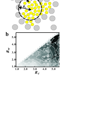
Figure 6: (Color online.) (a) Schematic showing a group of small particles temporarily confined within a region bounded by large particles. Each small particle is assigned a value $R_{w}$ which is its closest distance to any large particle (the large particles act as “walls”). Within each region, the local maximum of $R_{w}$ identifies the “confinement pore size” $R_{c}$ for that region. Thus, $R_{c}$ is the maximum radius of a circle that fits within the bounded region. (b) A contour plot for the mean square displacement $\langle\Delta r^{2}\rangle$ (at fixed $\Delta t=\Delta t^{*}$) as a function of the effective pore size $R_{c}$ where the given particle is located, and the distance of that particle from the nearest “wall” $R_{w}$, for state E with $\phi=0.66$. Darker shading corresponds with high mobility. The motion of particles is faster in larger pores (large $R_{c}$) and when further from the walls (larger $R_{w}$ for a constant $R_{c}$). The length scales are in terms of the small particle diameter. For these data, $R_{c}^{*}=3.6$; only 10% of regions have $R_{c}>R_{c}^{*}$.

Next, we consider the relationship between the confinement effects and mobility in large size ratio systems. The confinement effects are composed of both confinement size effects and confinement surface effects. For confined colloidal suspensions, particle motion was slower in more confined spaces, but there was not a strong influence from the confining surfaces Nugent . Numerical simulations show that the particles move slowly near rough walls, and quickly near smooth walls Kob3 . We thus wish to distinguish between finite size effects and interfacial effects. First, we define clusters of large particles as those large particles separated by a distance less than $1.4\sigma_{L}$, and these clusters form “walls” surrounding small particles. In some cases, a connected cluster of large particles completely surrounds a group of small particles, as sketched in Fig. 6. Within such a region, we compute the distance $R_{w}$ from each small particle to the nearest “wall” particle. The maximum value of $R_{w}$ within the confined region defines $R_{c}$, the effective “confinement pore size.” $R_{w}$ and $R_{c}$ are indicated in Fig. 6(a). $R_{w}$ is calculated per small particle, and $R_{c}$ per pore; both of these are functions of time. The dependence of specific particles’ behaviors on $R_{w}$ should give insight into interfacial effects, and the dependence of pore-averaged behavior on $R_{c}$ should give a separate insight into finite size effects, although of course these two effects are likely both present simultaneously.

Figure 6(b) shows a contour plot of $\langle r^{2}\rangle$ as a function of a ($R_{w}$, $R_{c}$) plane at state E and $\phi$ = 0.66. The results are located only at the lower right of the graph as $R_{c}\geq R_{w}$ from our definitions. The darker region at the upper right corresponds to high $\langle r^{2}\rangle$, showing that the mobility increases inside large pores (large $R_{c}$) and far from walls (large $R_{w}$). Given the incommensurate sizes of the large and small particles, it is difficulty for small particles to pack well near the “walls” [see Fig. 5(c)] and so not surprisingly our results are consistent with simulated rough walls Kob3 . There is also a slight gradient of increasing mobility as a function of pore size $R_{c}$ for fixed $R_{w}<1.5$, indicating that there is a finite size effect in addition to an interfacial effect. That is, smaller pores (smaller $R_{c}$) have more particles close to the pore walls, and thus experience stronger interfacial effects, but the data indicate that the influence of the interface on adjacent particles is less within large pores.

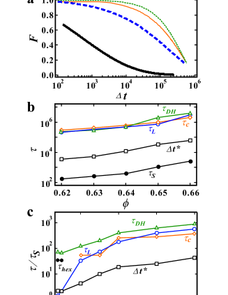
Figure 7: (Color online.) (a) The time dependence of $F(k,\Delta t)$ for small particles (thick solid (black) line; $k=2\pi/\sigma_{S}$) and for large particles (thick dashed (blue) line; $k=2\pi/\sigma_{L}$) at state E and $\phi$ = 0.66. The thin solid (red) line indicates the breakup of the largest confined regions, and the thin dashed (green) line indicates when the most mobile particles become less mobile. (b) The typical structural relaxation time $\tau_{S}$ for small particles (filled circles), the structural relaxation time $\tau_{L}$ for large particles (open circles), the confinement lifetime $\tau_{c}$ (diamonds), the dynamical heterogeneity lifetime $\tau_{DH}$ (triangles), and the peak time for the non-Gaussian parameter $\Delta t^{*}$ (squares). The data are for state E. (c) Five time scales ($\tau_{L}$, $\tau_{c}$, $\tau_{DH}$, $\Delta t^{*}$, and $\tau_{hex}$) normalized by $\tau_{S}$ as a function of $\sigma_{L}/\sigma_{S}$ at $\phi_{L}/\phi_{S}$ = 2.0 at $\phi$ = 0.66. $\tau_{hex}$ is the lifetime of hexagonal order and corresponds to the filled hexagon symbols. (These data go through state points A, C, and E; see Fig. 2.) (d) Five time scales ($\tau_{L}$, $\tau_{c}$, $\tau_{DH}$, $\Delta t^{*}$, and $\tau_{hex}$) normalized by $\tau_{S}$ as a function of $\sigma_{L}/\sigma_{S}$ at $\phi_{L}/\phi_{S}$ = 0.5 at $\phi$ = 0.66. (These data go through state points B, D, and F.) There are only a few confinement regions when $\sigma_{L}/\sigma_{S}<1.5$, preventing a clear determination of $\tau_{c}$, so those curves are clipped in (c) and (d).

To obtain further evidence for the relationship between the confinement effects and dynamical heterogeneity, we also investigate the temporal relationship between local structures and dynamical heterogeneity. We calculate the intermediate function $F(k,\Delta t)$ for small and large particles separately at fixed $k$ = 2$\pi/\sigma_{S}$ for small particles (thick solid (black) line in Fig. 7(a)) and $k$ = 2$\pi/\sigma_{L}$ for large particles (thick dashed (blue) line in Fig. 7(a)). The structural relaxation time scales for small and large particles, $\tau_{S}$ and $\tau_{L}$, are set by $F(k,\tau)$ = 1/e. We next consider all of the confined regions and the distribution of region sizes $R_{c}$. We determine the distribution of all pore sizes $R_{c}$ (taken over the entire simulation run), and find the threshold size $R_{c}^{*}$ for the top 10% of this distribution. For each pore at each time, we define $W_{c}(t)=1$ if $R_{c}(t)>R_{c}^{*}$ and $W_{c}(t)=0$ otherwise. Typical values of $R_{c}$ range from 2.8 to 5.6. The temporal correlations of the regions are given by $\langle W_{c}(\Delta t)\cdot W_{c}(0)\rangle/\langle W_{c}(0)^{2}\rangle$, plotted as the thin solid (red) line in Fig. 7(a). The typical lifetime of large regions is given as $\tau_{c}$ where the correlation drops to $1/e$. Similarly, for each particle we define a parameter $W_{DH}$ which is equal to 1 if the particle’s displacement $\Delta r$ at that time is within the top 10% of the displacement distribution, and 0 otherwise. The correlation $\langle W_{DH}(\Delta t)\cdot W_{DH}(0)\rangle/\langle W_{DH}(0)^{2}\rangle$ is plotted as the thin dashed (green) line in Fig. 7(a), and $\tau_{DH}$ is defined by the $1/e$ time again; this is the time scale over which particles exchange between being fast and slow, as mentioned in the Introduction.

Figure 7(b) shows the $\phi$ dependence of these four time scales ($\tau_{S}$, $\tau_{L}$, $\tau_{c}$, $\tau_{DH}$ and $\Delta t^{*}$). The fastest time scale is $\tau_{S}$ (filled circles), and the large particles are much slower ($\tau_{L}$, open circles). What is more notable is that $\tau_{L}\approx\tau_{c}$, in other words, large particle motions relate to the relaxation of confined regions. This is further evidence that the large particles form walls. Furthermore, $\tau_{c}\approx\tau_{DH}$ is observed, connecting the confinement-induced dynamics with the dynamically fast particles. Faster particles exchange identities with slower particles when the confining walls rearrange.

If the spatial dynamical heterogeneity is actually induced by the confinement effect, we would expect to see $\tau_{L}\approx\tau_{c}\approx\tau_{DH}$, and the correspondence should be strongest for large size ratio systems. Figure 7(c) and (d) show these time scales normalized by $\tau_{S}$ as a function of the size ratio $\sigma_{L}/\sigma_{S}$ at $\phi_{L}/\phi_{S}$ = 2.0 and 0.5, respectively; the data are for $\phi=0.66$. Indeed, for $\sigma_{L}/\sigma_{S}\geq 1.5$, we find $\tau_{L}$ is similar to $\tau_{c}$ and $\tau_{DH}$. Not surprisingly, the relaxation time scale $\tau_{c}$ for the confinement effect is governed by the relaxation time $\tau_{L}$ for the large particles which define the pores; more significantly, the lifetime of dynamically heterogeneous regions is also connected to the behavior of the large particles.

On the other hand, we find $\tau_{L}/\tau_{S}\rightarrow 1$ when $\sigma_{L}/\sigma_{S}\rightarrow 1$, which is to be expected. In these cases, $\tau_{DH}$ remains large, showing that here the dynamical heterogeneity is less influenced by the relaxation of the large particles. However, $\tau_{DH}$ is same order as the lifetime of hexagonal order, as seen in Fig. 7(c,d) by comparing the triangles ($\tau_{DH}$) with the filled hexagons ($\tau_{hex}$). This new time scale, $\tau_{hex}$, is defined in a similar way as the other time scales: particles with $\psi_{6}>0.8$ are considered hexagonal, and the correlation time for having $\psi_{6}>0.8$ is $\tau_{hex}$. This time scale is only relevant for samples with reasonable amounts of hexagonal order [compare Fig. 5(b,d)], and so is only shown for samples with small size ratios. (This is why it is not shown in Fig. 7(b) which has $\sigma_{L}/\sigma_{S}=2.5$.) It is further evidence that local hexagonal order influences the dynamics in similar size ratio systems. In these cases, the confinement effect is more likely due to hexagonal regions composed of both particle species, rather than networks formed by only the large particles, and thus $\tau_{c}$ becomes ill-defined and we do not show it in Fig. 7(c,d).

The competition between hexagonal ordering and crowding due to large particles likely accounts for the cases in Fig. 7(c,d) where $\tau_{DH}>\tau_{L}$. For example, states with $\sigma_{L}/\sigma_{S}=1.5$ still have regions of hexagonal ordering composed of both particle sizes. In these cases $\Theta$ is small [see Fig. 2(d)] and the confinement effect is weak. Another example where $\tau_{DH}>\tau_{L}$ is the state with $\sigma_{L}/\sigma_{S}=3.0$, $\phi_{L}/\phi_{S}=0.5$ [Fig. 7(d)]. The large particles are scarce, but result in a strong confinement influence; however, the more numerous small particles can themselves form hexagonal patches, influencing their mobility. We expect that for 3D glass-formers, local crystalline order is much less significant, and so confinement effects would more strongly determine $\tau_{DH}$ in all cases.

Furthermore, we consider the relationship among $\Delta t^{*}$ and other time scales (Fig. 7(c) and (d)). As a reminder, $\Delta t^{*}$ is the time scale at which the small particle displacement distribution is the most non-Gaussian. This time scale is used to define the mobility of particles and so is part of the definition of a “mobile” particle and thus $\tau_{DH}$. $\Delta t^{*}>\tau_{S}$ shows that small particles move appreciable distances during the time $\Delta t^{*}$. That is, the non-Gaussian displacements are over significant distances, enough to relax the small particle structure, and this becomes more true at larger size ratios, although this motion is all localized within a region defined by nearby large particles. In all cases $\tau_{DH}>\Delta t^{*}$ showing that slow and fast regions do not change identities with each particle rearrangement, but rather take longer times to change. Particles may rearrange several times confined within a large pore (several $\Delta t^{*}$) before the pore rearranges and the particles change their mobility. An important caveat is that these observations are for the average behavior of particles, and we are not implying that the connections between pore sizes and dynamics are strongly deterministic. Nonetheless the hierarchy of time scales in Fig. 7 is suggestive of nontrivial connections between the spatial arrangements of the large particles and the long-lived lifetimes of dynamically unusual regions, both fast and slow.

III.3 Aging

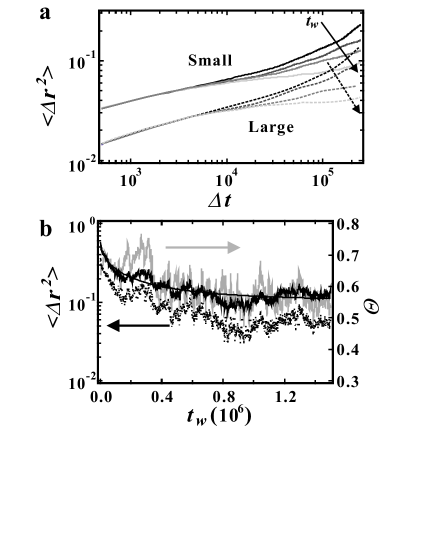
Figure 8: (a) $\langle\Delta r^{2}\rangle$ as a function of lag time $\Delta t$ for small particles (solid lines) and for large particles (dashed lines) at $t_{w}=10^{3},10^{4},10^{5}$ and $10^{6}$ at state E and $\phi$ = 0.72. The mobility of both particle species decreases with respect to aging time. (b) The dark black lines correspond to $\langle\Delta r^{2}\rangle$ at $\Delta t=10^{5}$ as a function of aging time $t_{w}$ for small particles (solid) and large particles (dashed). The smooth curves are fits with a stretched exponential, and we find that the decay time of large particles is slightly shorter than that of small particles. The gray line show the waiting time dependence of $\Theta$, the correlation between the displacements of a large particle and its surrounding small particles. The choice of $\Delta t=10^{5}$ is arbitrary although panel (a) shows that this is a reasonable choice to capture the slowing dynamics.

Next we investigate aging dynamics in binary samples with large size ratios. We study state E at $\phi=0.72$ where it is in a glassy state ($\phi_{g}\sim 0.68$ for this state). Figure 8(a) shows $\langle\Delta r^{2}\rangle$ for small and large species separately at waiting times $t_{w}=10^{3},10^{4},10^{5}$ and $10^{6}$. At short time scales ($\Delta t<5000$), $\langle\Delta r^{2}\rangle$ is independent of $t_{w}$. Particles move within cages formed by their nearest neighbor particles. At longer time scales $\Delta t>5000$, $\langle\Delta r^{2}\rangle$ increases as the cages rearrange and allow particles to move to new positions. This upturn in $\langle\Delta r^{2}\rangle$ decreases with increasing $t_{w}$, indicating the aging of the system, similar to what has been seen in experiments courtland03 ; Gianguido ; Jenn . Figure 8(b) shows the $t_{w}$ dependence of $\langle\Delta r^{2}\rangle$ at fixed $\Delta t$ = 10⁵. Though the results at small $t_{w}$ ($t_{w}<\Delta t$) are hard to interpret as the dynamics change during $\Delta t$, we can observe the clear temporal change of $\langle\Delta r^{2}\rangle$ for both particle species. For “old” systems, the plateau of $\langle\Delta r^{2}\rangle$ extends over a large range of time scales, with the plateau height corresponding to the cage size. Within our uncertainty, the large and small particles age almost at the same rates, as suggested by the similar shapes of $\langle\Delta r^{2}\rangle$ curves (Fig. 8(a)). Again, these observations are consistent with experiments in binary colloidal glasses Jenn .

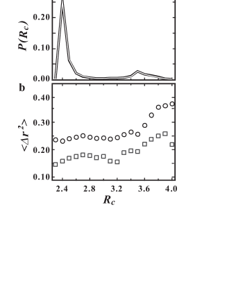
Figure 9: (a) The probability distribution $P(R_{c})$ of confinement pore sizes at $t_{w}=10^{3}$ (black line) and $t_{w}=10^{6}$ (superimposed white line), showing the distributions are essentially identical. This is for state E with $\phi=0.72$. (b) Mean squared displacements $\langle\Delta r^{2}\rangle$ for fixed $\Delta t=10^{5}$ as a function of the confinement pore size $R_{c}$ at $t_{w}=10^{3}$ (circles) and $t_{w}=10^{6}$ (squares), for the same state as (a). The upward trend (faster motion for larger pores) is similar to what is seen in equilibrated liquids [Fig. 6(b)]. For these data $\Delta t=10^{5}$ to capture time scales over which the dynamics age [see Fig. 8(b)].

We wish to know a reason for the slowing dynamics with respect to the waiting time. First, we confirm that the overall structure is unchanged with age: we compute the pair correlation function $g(R)$ at $t_{w}$ = 1000 and 10⁶ and cannot observe any difference between them, similar to prior observations in simulations kob00 and experiments Gianguido ; Jenn . $g(R)$ is a spatial average over the whole system, so we next consider the relation between local structure and local mobility. We use the confinement pore size $R_{c}$ to characterize the local structure of the particles within a given confining region. Figure 9 shows $\langle\Delta r^{2}\rangle$ and the probability distribution $P(R_{c})$, both as functions of $R_{c}$ at $t_{w}$ = 1000 and 10⁶. We find that $P(R_{c})$ does not change at all and this is further evidence that the structure does not change. However, the mobility decreases with age with the dependence on $R_{c}$ relatively unchanged other than the amplitude. This implies that the mobility decrease is not due to local structural changes, but rather an average slowing of the whole system Gianguido .

Next, we focus on the importance of confinement which strongly influences the dynamics of our equilibrated large size ratio binary systems. As noted above, the confinement strength depends on the confinement size $R_{c}$ and the effective rigidity of the walls, that is, $\Theta$. In aging systems, $P(R_{c})$ does not change with respect to $t_{w}$, but $\Theta$ could depend on $t_{w}$ since $\Theta$ is a dynamical property rather than a structural property. We compute $\Theta(t_{w})$ at fixed $\Delta t$ = 10 ⁵, shown as the gray line in Fig. 8(b). The behavior of $\Theta$ looks similar to the mobility change of both particles. Figure 10 shows a scatter plot of the mean square displacement $\langle\Delta r^{2}\rangle$ as a function of $\Theta$, for all large particles and all waiting times $t_{w}$. We can clearly see the correlation between the mobility and $\Theta$. When $\Theta$ decreases, the cooperative motion between small and large particles is less, in other words, the rigidness of walls increases. This result implies that confinement effects become stronger during aging and it may help explain the slowing down of the mobility. However, we don’t know why $\Theta$ decreases as the sample ages.

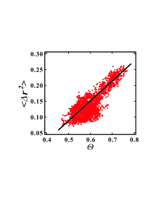
Figure 10: (Color online.) Scatter plot of the mean square displacement $\langle\Delta r^{2}\rangle$ as a function of $\Theta$ at state E and $\phi$ = 0.72, using $\Delta t=10^{5}$. Each point corresponds to a different $t_{w}$, the time since the start of the simulation. The solid line is a least squares fit. The data indicate that mobility is linked to the correlation of the motion between large particles and their nearest neighbors.

IV Conclusion

We have examined the glass transition in binary mixtures with a large size ratio, finding results that are distinct from binary mixtures with smaller size ratios. Systems with smaller size ratios are often studied, and the utility of using two particle sizes in those cases is to frustrate the packing and prevent crystallization. Crystals are also frustrated in our simulations with large size ratios, and in addition we find several new results. First, we have investigated fragility of binary systems. The fragility of binary systems with size ratios close to 1 ($\sigma_{L}/\sigma_{S}<1.4$) is related to the growth of ordered regions: more fragile liquids show dramatic increases in hexagonal order as the glass transition is approached KAT ; Sun ; Coslovich . However, systems with larger size ratios do not show this relation. Both types of systems have fragilities which are related to the growth of a dynamical length scale $\xi$, although the sign of this correlation is opposite for the small and large size ratio systems.

The data show that in large size ratio systems, large particles act as quasi-immobile walls which confine the small particles and slow the dynamics overall. The large particles define regions with a range of sizes. Small particles in large regions find it easier to move, even if within that region they may be adjacent to a large particle at the boundary of the region. Small particles in smaller regions are much less mobile. In addition to these finite size effects, there are interfacial effects: small particles near large particles move slower than those farther away. Those results are what is often seen in experiments and simulations of confined supercooled liquids. Furthermore, as is often observed in simulations and experiments, we find some particles are unusually mobile. Our new observation is that the length of time which these particles stay unusually mobile is connected to the lifetime of the confinement effect and thus the relaxation time of the large particles.

Finally, we also investigate aging dynamics in large size ratio systems. Below the glass transition, the mobility decreases with respect to the waiting time, though we cannot observe any structural change. We find that in “younger” systems that the motion of large particles is correlated with the motion of their neighbors, but that in “older” systems this correlation is markedly smaller. This correlation (or lack of it) relates to the confinement effect, suggesting that the large particles become more rigid confiners in older samples.

It is important to note that simulations of softer particles with a charged (Yukawa) potential find results different from ours, pointing out that our results are not completely generalizable. In simulations with a size ratio $1:5$, the large particles crystallized kikuchi07 . In these cases, the large particles did not rearrange but rather moved on their lattice sites, and small particles could only move by diffusive hopping motions between the crystal interstices. This is in contrast to our simulations where the large particles are always able to rearrange (albeit more slowly than the small particles).

Overall, our results suggest that in binary soft sphere systems, the effect of the large particles to induce finite size effects within the sample play an interesting role in the dynamics. Two relevant variables are the finite sizes of regions between large particles, and the effective rigidity of the large particles. While our simulation studies 2D systems, the results are similar to prior observations in 3D binary colloidal experiments Jenn ; Narumi with moderate size ratios. While the effects are easiest to see with large size ratios, one implication of our simulations is that these effects may be relevant although less obvious in binary systems of smaller size ratios. Indeed, one of the goals of our simulations was to understand the effect of structure by using systems where structural heterogeneity is more obvious. These results may also have implications for studies of nanocomposites, where inclusions into polymer glasses can dramatically affect the properties of materials Rittigstein ; Kropka .

References

- (1) P. G. Debenedetti and F. H. Stillinger, Nature 410, 259 (2001).
- (2) C. A. Angell, J. Non-Cryst. Solids 13, 131 (1991).
- (3) C. A. Angell, Science 267, 1924 (1995).
- (4) M. D. Ediger, C. A. Angell and S. R. Nagel, J. Phys. Chem. 100, 13200 (1996).
- (5) J. Horbach, W. Kob and K. Binder, Philos. Mag. B 320, 235 (1998).
- (6) R. M. Ernst, S. R. Nagel, and G. S. Grest, Phys. Rev. B 43, 8070 (1991).
- (7) A. van Blaaderen and P. Wiltzius, Science 270, 1177 (1995).
- (8) W. Kob, C. Donati, S. J. Plimpton, P. H. Poole, and S. C. Glotzer, Phys. Rev. Lett. 79, 2827 (1997).
- (9) C. Donati, J. F. Douglas, W. Kob, S. J. Plimpton, P. H. Poole, and S. C. Glotzer, Phys. Rev. Lett. 80, 2338 (1998).
- (10) M. D. Ediger, Annu. Rev. Phys. Chem. 51, 99 (2000).
- (11) E. R. Weeks, J. C. Crocker, A. C. Levitt, A. Schofield and D. A. Weitz, Science 287, 627 (2000).
- (12) M. M. Hurley and P. Harrowell, Phys. Rev. E 52, 1694 (1995).
- (13) L. Berthier et al., Science 310, 1797 (2005).
- (14) R. Yamamoto and A. Onuki, J. Phys. Soc. Jpn. 66, 2545 (1997).
- (15) C. A. Angell, K. L. Ngai, G. B. McKenna, P. F. McMillan, and S. W. Martin, J. Appl. Phys.88, 3113 (2000).
- (16) I. M. Hodge, Science 267, 1945 (1995).
- (17) W. van Megen, T. C. Mortensen, S. R. Williams, and J. Muller, Phys. Rev. E 58, 6073 (1998).
- (18) R. E. Courtland and E. R. Weeks, J. Phys.: Condens. Matt. 15, S359 (2003).
- (19) G. C. Cianci, R. E. Courtland and E. R. Weeks, Solid State Commun. 139, 599 (2006).
- (20) J. M. Lynch, G. C. Cianci and E. R. Weeks, Phys. Rev. E 78, 031410 (2008).
- (21) T. Hamanaka and A. Onuki, Phys. Rev. E 74, 011506 (2005).
- (22) T. Kawasaki, T. Araki and H. Tanaka, Phys. Rev. Lett. 99, 215701 (2007).
- (23) M. Sun, Y. Sun, A. Wang, C. Ma, J. Li, W. Cheng and F. Liu, J. Phys.:Condens. Matter 18, 10889 (2006).
- (24) D. Coslovich and G. Pastore, J. Chem. Phys. 127, 124504 (2007).
- (25) F. Sausset, G. Tarjus and P. Viot, Phys. Rev. Lett. 101, 155701 (2008).
- (26) E. R. Weeks and D. A. Weitz, Phys. Rev. Lett. 89, 095704 (2002).
- (27) A. Widmer-Cooper, P. Harrowell, and H. Fynewever, Phys. Rev. Lett. 93, 135701 (2004).
- (28) A. Widmer-Cooper and P. Harrowell, J. Phys.: Condens. Matt. 17, S4025 (2005).
- (29) A. Widmer-Cooper, H. Perry, P. Harrowell, and D. R. Reichman, Nature Phys. 4, 711 (2008).
- (30) J. C. Conrad, F. W. Starr, and D. A. Weitz, J. Phys. Chem. B 109, 21235 (2005)
- (31) G. S. Matharoo, M. S. G. Razul, and P. H. Poole, Phys. Rev. E 74, 050502 (2006).
- (32) L. Berthier and R. L. Jack, Phys. Rev. E 76, 041509 (2007).
- (33) G. A. Appignanesi and J. A. R. Fris, J. Phys.: Condens. Matt. 21, 203103 (2009).
- (34) A. Imhof and J. K. G. Dhont, Phys. Rev. Lett. 75, 1662 (1995).
- (35) A. D. Dinsmore, A. G. Yodh, and D. J. Pine, Phys. Rev. E 52, 4045 (1995).
- (36) S. Asakura and F. Oosawa, J. Chem. Phys. 22, 1255 (1954).
- (37) J. C. Crocker, J. A. Matteo, A. D. Dinsmore, and A. G. Yodh, Phys. Rev. Lett. 82, 4352 (1999).
- (38) A. J. Moreno and J. Colmenero, Phys. Rev. E 74, 021409 (2006).
- (39) T. Voigtmann and J. Horbach, Phys. Rev. Lett. 103, 205901 (2009).
- (40) P. N. Pusey and W. van Megen, Nature 320, 340 (1986).
- (41) T. Gleim, W. Kob, and K. Binder, Phys. Rev. Lett. 81, 4404 (1998).
- (42) G. Szamel and E. Flenner, Europhys. Lett. 67, 779 (2004).
- (43) M. Tokuyama, Physica A 378, 157 (2007).
- (44) J. D. Weeks, D. Chandler and H. C. Andersen, J. Chem. Phys. 54, 5237 (1971).
- (45) B. I. Halperin and D. R. Nelson, Phys. Rev. Lett. 41, 121 (1978).
- (46) N. Kikuchi and J. Horbach, Europhys. Lett. 77, 26001 (2007).
- (47) B. Schiener et al. J. Mol. Liq. 69, 243 (1996).
- (48) G. Brambilla, et al., Phys. Rev. Lett. 102, 085703 (2009).
- (49) D. El Masri, et al., J. Stat. Mech. 2009, P07015 (2009).
- (50) R. L. Cook et al. J. Chem. Phys. 100, 5178 (1994).
- (51) H. Tanaka, J. Phys.: Cond. Mat. 10, L207 (1998).
- (52) R. Kurita and H. Tanaka, Phys. Rev. Lett. 95, 065701 (2005).
- (53) T. Hecksher, A. I. Nielsen, N. B. Olsen, and J. C. Dyre, Nat. Phys. 4, 737 (2008).
- (54) A. Donev, F. H. Stillinger and S. Torquato, J. Chem. Phys. 127, 124509 (2007).
- (55) B. Doliwa and A. Heuer, Phys. Rev. E 61, 6898 (2000).
- (56) E. R. Weeks, J. C. Crocker and D. A. Weitz, J. Phys.: Cond. Mat. 19, 205131 (2007).
- (57) A. Rahman, Phys. Rev. 136, A405 (1964).
- (58) P. Scheidler, W. Kob, and K. Binder, Europhys. Lett. 52, 277 (2000); 59, 701 (2002).
- (59) C. R. Nugent, K. V. Edmond, H. N. Patel and E. R. Weeks, Phys. Rev. Lett. 99, 025702 (2007).
- (60) K. Kim, Europhys. Lett. 61, 790 (2003).
- (61) M. Alcoutlabi and G. B. McKenna, J. Phys.: Condens. Matt. 17, R461 (2005).
- (62) T. Narumi, S. V. Franklin, K. V. Desmond, M. Tokuyama and E. R. Weeks, arXiv:0911.0702.
- (63) W. Kob, J.-L. Barrat, F. Sciortino, and P. Tartaglia, J. Phys: Cond. Matt. 12, 6385 (2000).
- (64) P. Rittigstein, R. D. Priestley, L. J. Broadbelt, and J. M. Torkelson, Nature Materials 6, 278 (2007).
- (65) J. M. Kropka, V. Pryamitsyn, and V. Ganesan, Phys. Rev. Lett. 101, 075702 (2008).