Efficient equilibrium sampling of all-atom peptides using library-based Monte Carlo

Abstract

We applied our previously developed library-based Monte Carlo (LBMC) to equilibrium sampling of several implicitly solvated all-atom peptides. LBMC can perform equilibrium sampling of molecules using the pre-calculated statistical libraries of molecular-fragment configurations and energies. For this study, we employed residue-based fragments distributed according to the Boltzmann factor of the OPLS-AA forcefield describing the individual fragments. Two solvent models were employed: a simple uniform dielectric and the Generalized Born/Surface Area (GBSA) model. The efficiency of LBMC was compared to standard Langevin dynamics (LD) using three different statistical tools. The statistical analyses indicate that LBMC is more than 100 times faster than LD not only for the simple solvent model but also for GBSA.

Department of Computational Biology, School of Medicine, University of Pittsburgh, Pittsburgh, Pennsylvania 15260

1 Introduction

Conformational fluctuations in proteins are well appreciated to be essential to biochemistry, in roles accompanying binding, catalysis and locomotion [1]. In recent years, the importance of fluctuations has been further underscored by recognition of the widespread presence of disordered regions in proteins [2, 3]. Structural experiments, however, are fairly limited in their power to characterize such fluctuations from a true ensemble perspective. For a given protein, X-ray crystallography generates one or a very small number of configurations, typically excluding the most flexible regions [4, 5]. NMR studies yield highly approximate structure sets based on simplified forcefields and non-canonical algorithms [6]. Cryo-EM can characterize large structural fluctuations but at low resolution [7].

In principle, computations are ideal for characterizing fluctuations in biomolecules, but sampling power is typically inadequate except for small systems. The basic reason is the well-known gap in timescales between simulation and biological behavior [8]. To bridge this gap, much effort has been undertaken in the field to develop new efficient sampling techniques. Many of these techniques are based on “generalized ensembles” including replica exchange [9, 10, 11, 12]. Other techniques use modified energy surfaces [13, 14, 15] or modified dynamics [16, 17, 18, 19, 20]. The “resolution exchange” (ResEx) algorithm uses a ladder of different resolution models with occasional exchanges between levels [21]. Both replica-exchange and ResEx can be implemented in the serial top-down scheme [22, 23].

Another strategy for speeding calculations is to exploit computer memory to store frequently used information. In particular, libraries of molecular fragment configurations can be stored and re-used. Libraries were previous used by Rosetta [24], but not for true canonical sampling. In our previous work we introduced the statistical rigorous library based Monte Carlo (LBMC) and used it to incorporate atomic details into a coarse-grained protein model at a small computational cost [25]. The semi-atomistic model was applied to equilibrium sampling of several proteins containing up to 309 residues. LBMC was also applied to equilibrium sampling of several peptides described by OPLS-AA forcefield [26] with a simple uniform dielectric model to model the solvent [25]. A large efficiency gain of LBMC compared to standard Langevin dynamics was observed. Inspired by the results of our previous study , here we further investigate the application of LBMC to equilibrium sampling of all-atom peptides.

In this study we apply LBMC to several implicitly solvated peptides described by OPLS-AA forcefield with two different implicit solvent models: a simple uniform dielectric of 60 and the Generalized Born/Surface Area (GBSA) model [27]. The efficiency of LBMC was quantified by comparison to Langevin Dynamics using three different statistical tools. The first tool is based on the autocorrelation behavior of the end-to-end distance, the second uses our previously developed “decorrelation time” analysis [28] , and the third employs a block averaging analysis [29] of the end-to-end distances. All the analyses point to efficiency gains of two to three orders of magnitude in the three peptides studied - tetraalanine, octaalanine and Met-enkephalin.

2 Methods

2.1 Library-based Monte Carlo Method (LBMC)

The library-based Monte Carlo (LBMC) method was recently introduced, along with complete derivations [25]. Here we briefly review the method.

LBMC uses the simple idea to divide a molecule into non-overlapping fragments, each of which is pre-sampled into a library of Boltzmann-distributed fragment configurations. For peptides and proteins, fragments based on amino acids are natural. Trial moves consist of swapping the present configuration of one or more fragments with members of the corresponding libraries. LBMC, which is a rigorous MC scheme , has several noteworthy features. (i) Libraries – e.g., for each amino acid – are generated one time and can be re-used in multiple simulations; accordingly, the internal-to-fragment interactions are never calculated during a simulation, saving some CPU cost. (ii) Because fragment configurations are pre-sampled based on all interactions internal to the fragment, those energy terms do not enter the Metropolis acceptance criterion. (iii) Perhaps most importantly, the complex correlations among degrees of freedom internal to a fragment are fully accounted for in the library-generation stage – i.e. , the “price” for the internal timescales is paid in advance.

A Metropolis-Hastings criterion for an LBMC trial move is derived in the usual way based on the detailed-balance condition [25]. In outline, the derivation is accomplished by first separating the full set of degrees of freedom $\vec{r}$ into $M$ fragments,$\overrightarrow{r}=\{\vec{r}_{1},...,\vec{r}_{M}\}$ . Similarly, the total energy of a forcefield $U^{\mathrm{{tot}}}$, which could include implicit solvent terms, is decomposed into components: the terms internal to each fragment $i$, denoted $U_{i}^{\mathrm{{frag}}}$, and all the “rest,” which are cross-fragment interaction terms lumped into $U^{\mathrm{{rest}}}$. Thus we have

$$U^{\mathrm{{tot}}}(\vec{r}_{1},...,\vec{r}_{M})=\sum U_{i}^{\mathrm{{frag}}}(\vec{r}_{i})+U^{\mathrm{{rest}}}(\vec{r}_{1},...,\vec{r}_{M})$$ (1)

In the present study, $U^{\mathrm{tot}}$ represent the OPLS-AA forcefield plus an implicit solvent model, as described below.

In our previous work, we derived Metropolis criteria for two types of library-swap trial moves [25]. The first is a simple swap move in which configurations from one or more fragments are swapped with configurations chosen uniformly from the corresponding libraries (Each library is already Boltzmann distributed according to $U_{i}^{\mathrm{{frag}}}$, as described below.) In the simple swap move, the generating probability for the trial/new configuration ($n$) is completely independent of the old configuration ($o$). This leads to significant cancellation of terms, and one finds the acceptance probability to be [25]

$$p_{\mathrm{{acc}}}(o\rightarrow n)=\min\left[1,\exp(-\beta\Delta U^{\mathrm{{rest}}})\right]$$ (2)

We will also employ a second type of swap move based on “neighbor lists.” In the context of LBMC a neighbor list is, for each configuration, the list of configurations deemed to be similar by an arbitrary criterion. The trial move of interest, then, is to choose a library configuration for swapping only among the neighboring configurations for a single fragment $i$. When trial configurations are selected uniformly among neighbors, it can be shown that the acceptance criterion is [25]

$$p_{\mathrm{{acc}}}(o\rightarrow n)=\min\left[1,\exp(-\beta\Delta U^{\mathrm{{rest}}})\frac{k_{i}^{o}}{k_{i}^{n}}\right]$$ (3)

where $k_{i}^{o}$ and $k_{i}^{n}$ are the number of neighbors of configuration $o$ and $n$ respectively for fragment $i$. If neighbor lists are constructed to have the same number of neighbors for all configurations in a given library, then the acceptance criterion of Eq. 3 reduces to Eq. 2.

Below we will explain our procedures for generating libraries and neighbor lists.

2.2 Practical library generation

The fragment used in this study correspond to individual amino acids, which are the natural building blocks of peptides. In previous LBMC work [25], we used both peptide planes and amino acids as fragments in separate simulations. However, amino acid fragments have the advantage of including detailed “Ramachandran correlations” among $\phi$ and $\psi$ angles, as well as the other degrees of freedom. In practical terms, this means that the timescales and correlations associated with Ramachandran effects are pre-sampled within the libraries.

Fragment configurations in the libraries were generated according to the Boltzmann factor of OPLSAA forcefield [26], plus the appropriate implicit solvent model, for all interactions internal to the fragment. Fragment libraries must include not only atomic coordinates, but also the six degrees of freedom necessary for connecting one fragment to the next. Full details of the degrees of freedom for amino acid libraries were given in [30], our previous work. In brief, we used dummy atoms “borrowed” from the next fragment to facilitate sampling the coordinates necessary for connecting fragments. Interactions with dummy atoms were fully accounted for to yield the correct ensemble of the whole molecule – as can be seen in our results below.

Although library ensembles, in principle, can be generated using any canonical sampling scheme, we found it most convenient to use internal-coordinate Monte Carlo (ICMC). ICMC readily permits fixing degrees associated with the dummy atoms which we did not wish to vary. Our use of ICMC properly accounted for internal-coordinate Jacobians, which ensure that the distribution obtained agrees with that from using the (natural) Cartesian coordinates. The standard Jacobians were employed – i.e., $r^{2}$ for bond lengths $r$ and $\sin\theta$ for bond angles $\theta$.

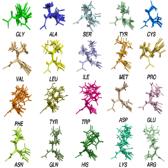
For each amino acid fragment, ICMC was run for $10^{9}$ steps to produce libraries of $10^{5}$ configurations. See Figure 1. The library configurations may not be fully statistically independent, but we do carefully assess the statistical quality of the ultimate ensembles of the full molecule – as shown below.

2.3 Neighbor-list construction

In LBMC, “neighbor lists” of library configurations similar to each library member provide a conveninent way to attempt relatively local moves in configuration space. As explained in our initial derivation [25], neighbors can be defined in an arbitrary way. Natural choices include criteria based on a pairwise “distance” similarity metric such as the root mean square deviation (RMSD) or the sum of absolute differences over all bond and dihedral angles in a given fragment as was used in our previous work [25]. When constructing neighbor lists, if configuration $i$ contains configuration $j$ in its neighbor list then $j$ must have $i$, to satisfy microscopic reversibility.

In the present work the neighbor lists were constructed to generate groups of $n=10$ similar configurations. To minimally perturb the molecule’s overall structure, similarity between two configs was quantified by the RMSD of six atoms, three at each end of the fragment. To construct neighbor lists, the following algorithm was used. A first “reference” structure is selected randomly from the whole library and the nearest $n-1$ configurations in the RMSD space are chosen for the first neighbor list. The next reference structure is randomly selected from the remaining configurations and again the closest $n-1$ configurations are chosen for this neighbor list. This process is repeated until the whole library is partitioned into equi-sized neighbor lists. In this study, each library has 10⁵ configurations and is partitioned into 10⁴ neighbor groups of size $n=10$.

In general, it is not necessary to make equal size clusters, nor is it necessary to strictly partition the whole library into “disconnected” neighbor lists. If there is a strict partitioning (as in the present study), then non-neighbor trial moves are required to ensure the possibility of ergodicity. By adjusting the fraction of local to global moves, the acceptance rate can be tuned. In the future, it will be worthwhile to construct and test overlapping (non-isolated) neighbor lists.

2.4 Efficiency analysis

It is critical to quantify the sampling quality of any new method, in comparison to a standard technique. In this study we assess the convergence of LBMC simulations and compare its efficiency relative to standard Langevin dynamics using three different statistical tools. One of these methods is semi-qualitative and the other two are quantitative.

Because there are no true physical timescales in our Monte Carlo simulations, our primary focus is to compare sampling efficiency in terms of single-processor wall-clock time. We recognize that different Langevin implementations (i.e., in different software packages) will vary in speed. However, we anticipate such differences will be small compared to the orders of magnitude efficiency we report below for LBMC. Furthermore, our reference Langevin simulations employ a low friction constant, which is recognized to improve sampling speed compared to a more physical water-like value [Paterlini1998].

The semi-qualitative tool we use to analyze sampling is the standard autocorrelation function of some slowly changing variable. The autocorrelation function is given, as usual, by

$$C_{x}(\tau)=\frac{\langle x(t)\;x(t+\tau)\rangle-\langle x\rangle^{2}}{\langle x^{2}\rangle-\langle x\rangle^{2}}$$ (4)

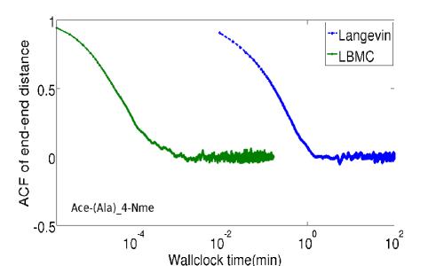
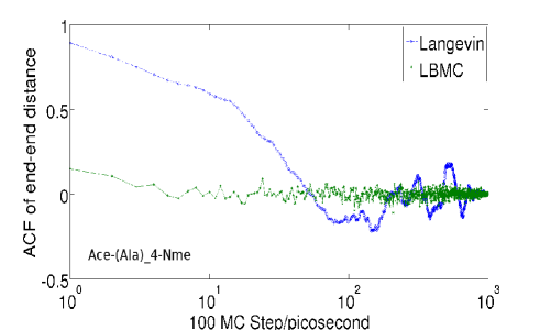
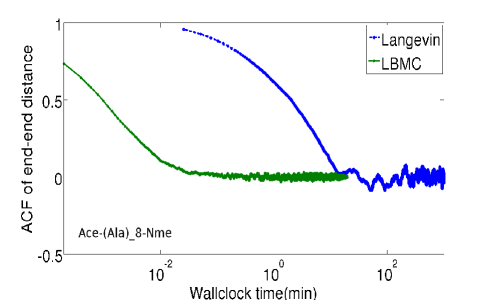
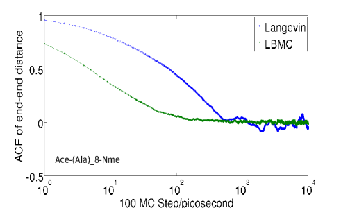
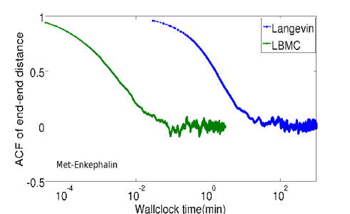
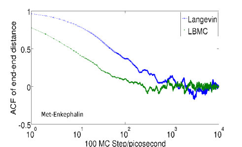
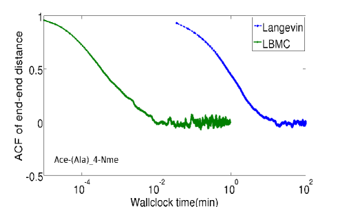
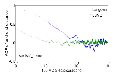
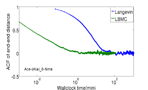
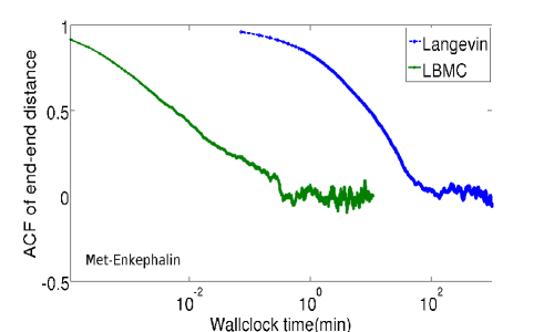
where $\langle x\rangle$ is the average value of $x(t)$, and $\tau$ is the time interval or number of MC steps between configurations in the trajectory. Because all correlations in an LBMC “trajectory” are sequential, a “time” correlation description is valid. A number of useful slow coordinates can be defined [31], and we choose the end-to-end distance of a peptide as a simple geometric measure which illustrates the key timescales. However, the auto-correlation behavior is not used to quantify efficiency in our study, but only to depict it graphically. We measured time in units of wall-clock minutes to facilitate comparison between LBMC and standard Langevin simulation.

The second statistical tool is based on our previously developed “structural de-correlation time” analysis which determines how much simulation time must elapse between configurations in the trajectory in order for them to exhibit statistical independence [28]. The ratio of the overall trajectory length to the decorrelation time provides an objective estimate of the effective sample size (ESS) – i.e., the number of independent configurations. Importantly, because all correlations are sequential in the LBMC Markov chain, the ESS for LBMC can be calculated from the same ratio of trajectory length to decorrelation time.

We therefore define the first efficiency factor as the gain in the sampling speed of LBMC over Langevin dynamics based on the ratio of CPU cost per independent configuration:

$$\hat{\gamma}_{1}=\frac{ESS_{\mathrm{\mathrm{LBMC}}}/t_{\mathrm{\mathrm{LBMC}}}}{ESS_{\mathrm{Langevin}}/t_{\mathrm{Langevin}}}$$ (5)

where $t_{\mathrm{LBMC}}$ and $t_{\mathrm{Langevin}}$ are the total wallclock times of LBMC and Langevin simulation respectively.

The last statistical method is based on the more traditional block averaging analysis [29, 32] of some slowly changing variable. In this approach, a trajectory is divided into “blocks” of different size. The mean value of the variable along with the standard error of the mean ($SE$) is calculated for different size blocks. As the block size increases, so does the standard error because blocks become more independent from each other. At some block size the standard error levels off, indicating that the blocks have become effectively independent from each other. This plateau is the true value of $SE$. We use block-averaging of the end-to-end distance, as a representative slow coordinate. We therefore define the second efficiency factor based on the ratio of CPU cost per “unit of precision”:

$$\hat{\gamma}_{2}=\frac{t_{\mathrm{Langevin}}SE_{\mathrm{Langevin}}^{2}}{t_{\mathrm{LBMC}}SE_{\mathrm{LBMC}}^{2}}$$ (6)

where $SE_{\mathrm{Langevin}}$ and $SE_{\mathrm{LBMC}}$ are the standard errors for Langevin and LBMC simulation, respectively, estimated from block averaging. Note that $SE^{2}$ is expected to vary linearly with inverse simulation time [32].

2.5 System and simulation details

We applied LBMC to three implicitly solvated peptides including Ace-(Ala)${}_{\text{4}}$-Nme, Ace-(Ala)${}_{\text{8}}$-Nme, and Met-enkephalin described by OPLS-AA forcefield [26]. No cutoffs were used in these relatively small systems. We chose these peptides because they have been extensively studied experimentally and computationally [33, 34, 35]. Two different implicit solvent models were employed: a uniform dielectric constant of $\varepsilon=60$ and the more standard GBSA model [27]. The constituent atomic radii for GBSA are taken from the OPLS-AA force field and the nonpolar solvation is calculated via the ACE approximation [36]. The Born radii used in GBSA are recomputed for every MC step.

For LBMC simulations of poly-alanine systems, three libraries were employed corresponding to Ace, Ala and Nme fragments. For Met-enkephalin (Tyr-Gly-Gly-Phe-Met), six libraries were used corresponding to Ace, Gly, Phe, Tyr, Met and Nme residues. Different libraries were used depending on the solvent models. For LBMC with uniform dielectric solvent we used fragment libraries sampled according to the uniform dielectric model, whereas for GBSA simulations we used libraries sampled according to GBSA solvent.

For all LBMC simulations reported here, the trial move was a single fragment swap with the corresponding library. For our systems, this was found to be the most efficient based on simulations with different number of fragments swapped per MC step. All system were sampled at 298 K.

For LBMC simulations of both solvent models Ace-(Ala)${}_{\text{4}}$-Nme was run for 10${}^{\text{5}}$ MC steps with configurations saved every 10 MC steps resulting into 10${}^{\text{4}}$ frames. Ace-(Ala)${}_{\text{8}}$-Nme was run for 10⁷ MC steps with frames saved every 100 MC steps resulting in 10${}^{\text{5}}$ structures. Met-enkephalin was run for 10⁶ MC steps with frames saved every 10 MC steps resulting into 10${}^{\text{5}}$ frames.

To compare LBMC with Langevin dynamics we ran LD simulations for the same three systems and both solvent models. Specifically, all three peptides were run for 100 ns with frames saved every picosecond resulting into 10${}^{\text{5}}$ structures. All Langevin simulations were run at the temperature of 298 K and the friction constant of 5 psec${}^{\text{-1}}$, as implemented in the Tinker software package [37].

3 Results

3.1 Ensemble Quality

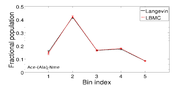
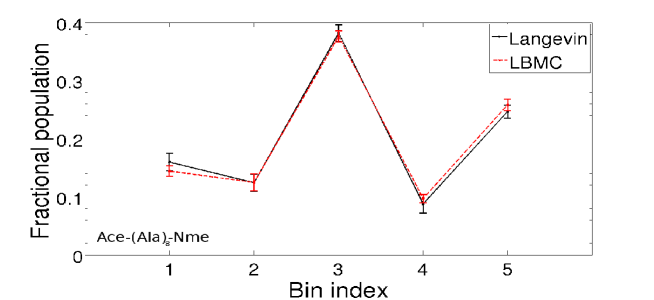
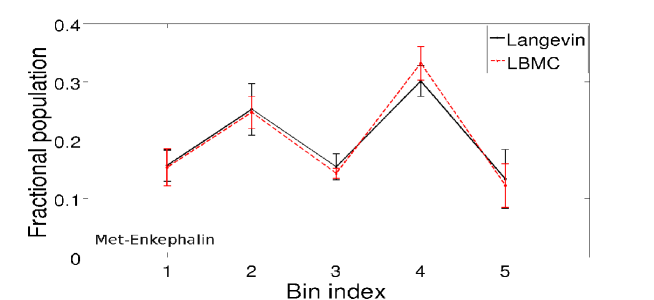
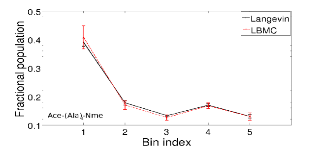
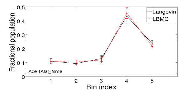
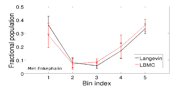
We first verified that LBMC samples the correct equilibrium distributions. For this purpose we prepared “structural bins” which are randomly selected regions of configuration space which cover the whole space, and can sensitively quantify sampling [38]. The bins were constructed using a Voronoi procedure as described in [30]. For all three systems we compared the fractional populations of the structural bins obtained from LBMC and Langevin simulations. The results for the uniform dielectric solvent model are shown in Figure 2 and for GBSA in Figure 3, indicating good agreement between two methods.

To examine the ensembles from a more traditional perspective, we also calculated hydrogen bond population and the helical content of octa-alanine. Based on the hydrogen-bond definition given in [19], we find the average number of hydrogen bonds in tetraalanine, octaalanine and Met-enkephalin to be ($2.400\pm 0.006$ , $5.00\pm 0.02$, $3.20\pm 0.01$) in the simple solvent model and ($2.84\pm 0.08$ , $6.63\pm 0.06$, $3.98\pm 0.07$) in GBSA from LBMC simulation. For comparison, we found ($2.408\pm 0.002$ , $5.03\pm 0.02$, $3.21\pm 0.01$) in simple solvent model and ($2.75\pm 0.08$ , $6.51\pm 0.06$, $4.06\pm 0.09$) in GBSA from Langevin simulation. Here the uncertainty is quantified as the standard error of mean of the number of hydrogen bonds in the specific ensemble. Helical content was defined to be the fraction of residues in the system whose $(\phi$, $\psi)$ dihedrals were within $\pm 25^{\circ}$ of the ideal angles of approximately $(-60^{\circ},-40^{\circ})$. We found helical population for octaalanine is $11.7\%(\pm 0.4\%)$ in the simple solvent model and $30\%(\pm 2\%)$ in GBSA from LBMC as compared $11.1\%(\pm 0.3\%)$ in simple solvent model and $31\%(\pm 2\%)$ in GBSA from Langevin simulation, respectively. These structural measures further verify our results.

3.2 Efficiency Analysis

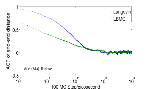
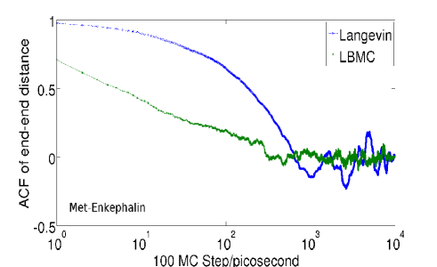
The efficiency of LBMC to sample the equilibrium distributions was compared to Langevin using the three statistical tools discussed in Sec. 2.4. The first tool is the autocorrelation function (ACF) of the end-to-end distance for each peptide. For all systems, the end-to-end distances was calculated based on coordinates of the methyl carbon atom of the Ace group and the methyl carbon of the Nme group. The autocorrelation function was calculated according to Eq. 4. As shown in Figures 4 and 5 , we calculated ACFs for all systems in the two solvent models and using two time measures. Most importantly, we depict the ACF vs. wallclock time, which suggests the high efficiency of LBMC compared to Langevin in these systems. For reference, we also computed each ACF as a function of the number of simulation steps.

The second statistical method is the “de-correlation time” analysis which we used to calculate the number of statistically independent configurations (i.e., the effective sample size ($ESS$)) in the trajectory [28]. The $ESS$ results for LBMC and Langevin simulations, along with the efficiency factors $\hat{\gamma}_{1}$ calculated using Eq. 5, are reported for the uniform dielectric model in Table 1 and for GBSA in Table 2. From Table 1 it follows that for the uniform dielectric model LBMC is more than three orders of magnitude faster than Langevin for Ace-(Ala)${}_{\text{4}}$-Nme, more than two orders of magnitude faster for Ace-(Ala)${}_{\text{8}}$-Nme and almost three orders of magnitude faster for Met-enkephalin. Table 2 indicates that for GBSA solvent LBMC is more than three orders of magnitude faster than Langevin for Ace-(Ala)${}_{\text{4}}$-Nme, over two order of magnitude faster for Ace-(Ala)${}_{\text{8}}$-Nme and over two orders of magnitude faster for Met-enkephalin. For Langevin simulations, the decorrelation time is also a physical timescale [28] as tabulated in Table 1 and Table 2: it is about 1nsec or less in the three peptides.

The third statistical tool is based on the more traditional block averaging analysis and we used it to confirm the efficiency results obtained from the previous method. We again employed the end-to-end distance which is a slowly changing variable. The standard errors ($SE$) of the mean for end-to-end distances from the block averaging, along with the efficiency factors $\hat{\gamma}_{2}$ calculated using Eq. 6, are reported for the uniform dielectric model in Table 1 and for GBSA in Table 2. Comparison of $\hat{\gamma}_{1}$ with $\hat{\gamma}_{2}$ indicates that the block averaging technique estimates similar efficiency factors to the de-correlation analysis, demonstrating the robustness of our analysis.

3.3 Regarding GBSA

GBSA affects both simulation cost (per timestep) and the ability to sample (by changing the landscape’s roughness). Both these factors, in turn, affect efficiency. The cost, however, is implementation specific. We now briefly address GBSA efficiency and implementation. For GBSA, the efficiency factors are slightly smaller than for the uniform dielectric model. When using GBSA solvent the ESS decreased by the factor of ca. 2.5 for both Langevin and LBMC. For LBMC the acceptance rate decreased as well. This indicates that sampling becomes more difficult for both methods in the more complicated energy landscape provided by GBSA. Note that all other parameters, such as the number of atoms and the number of steps, was the same for each method.

We can also compare solely the wallclock cost to run the same number of MC or Langevin steps for simple solvent model and GBSA. When GBSA solvent was employed, the simulation time increased by a factor of 4 for Langevin and by a factor of 6 for LBMC. The larger increase of the wallclock time for LBMC can be attributed to a relatively inefficient implementation of GBSA in our algorithm compared to the Tinker program. We therefore believe that the decrease of efficiency factors, $\hat{\gamma}_{1}$ and $\hat{\gamma}_{2}$, for GBSA simulations can be attributed to our inefficient implementation of GBSA rather than the difficulty of LBMC to sample complex energy landscapes. See further comments on GBSA in Sec. 4.

3.4 Neighbor-based trial moves

The use of neighbor swap moves in LBMC (Secs 2.1 and 2.3) is suggested by Tables 1 and 2, because the acceptance rate significantly dropped for LBMC simulations with GBSA solvent compared to the uniform dielectric model. To test the ability of neighbor-list trial moves to increase the acceptance rate for LBMC simulation of all-atom peptides, we employed two sets of trial moves: one with 30% and the other with 70% of local (neighbor-list) moves. Both sets helped to increase the acceptance rate. For example, for Ace-(Ala)${}_{\text{8}}$-Nme using 30% local moves increased the acceptance rate from 0.18 to 0.27 and 70% local moves led to 0.41. For Met-enkephalin 30% local moves increased the acceptance rate from 0.17 to 0.31 and 70% local moves led to 0.38. However, the efficiency analysis indicated that for simulations with local trial moves the efficiency factors $\hat{\gamma}_{1}$ and $\hat{\gamma}_{2}$ turned out to be smaller compared to simulations with regular (100% global) trial moves. As discussed in Sec 4, additional exploration of neighbor-list construction is needed.

4 Discussion

The initial results for sampling all-atom peptides in implicit solvent via LBMC are very encouraging. We wish to make some observations and also point out several avenues for improvement as well as some limitations.

First of all, LBMC is not simply internal-coordinate MC (ICMC) with “window dressing”. That is, using libraries is not merely a way to employ large trial moves, such as drastic changes to $\phi$ and $\psi$ dihedrals. Indeed if large dihedral moves are used in ICMC, the acceptance rate is over an order of magnitude smaller than for global swap moves in LBMC. The key to LBMC success (in the systems studied) is the correlated nature of trial moves: large $\phi$ and $\psi$ changes are accompanied, by construction, with correlated changes of other coordinates in the fragment (i.e., residue).

There appear to be two principal limitations for application of LBMC to all-atom sampling with standard forcefields. These limitations stem, in a sense, from the strength of LBMC for small flexible systems: extremely large trial moves (not feasible or physical in dynamics) lead to rapid sampling. For instance, LBMC will occasionally jump from one region of the Ramachandran plane to a completely different part. Such large moves immediately suggest that, first of all, LBMC with large trial moves will not be suitable for explicit solvent. Secondly, even in implicit solvent, once a single molecule becomes large and “dense” – such as a full protein – large-scale trial moves will again prove nearly impossible to accept.

We note that, in principle, LBMC is not limited to implicit solvent. In an explicit solvent simulation of a peptide, for example, trial moves for the peptides could be governed by LBMC and solvent moves via “ordinary” MC. In the LBMC acceptance criterion, $U^{rest}$ would include solvent interactions. Whether such an approach proves practical will depend sensitively on the construction of suitably local LBMC trial moves – i.e., crankshaft-like, see below. It is also possible that future methodologies will permit the conversion of implicit solvent ensembles to explicit solvent [39].

LBMC can however employ more “local” trial moves, for instance based on “neighboring” library configurations as described above. As noted in the Sec. 3, such local moves actually decrease sampling efficiency (despite increasing the acceptance ratio) in the small systems studied here. In larger systems, however, we expect neighbor-based moves to be helpful. Local moves should also prove important in sampling loops with LBMC. In the future, more sophisticated constructions of neighbor lists should be possible, as compared to our fairly simple approach described in Sec. 2.

Further improvements to GBSA-based sampling via LBMC appear to be possible, given our inefficient implementation of GBSA as discussed in Sec. 3. Indeed, generally speaking, GBSA is not well-suited to Monte Carlo simulation, as previously noted [40], because the non-pairwise energy terms depend on the entire molecule even when only part of it is changed as in typical MC trial moves. Therefore, other solvent models or approximations to GBSA [40, 41, 42] should improve LBMC efficiency further in terms of wall-clock time.

Like almost any canonical sampling method, LBMC can be employed in more sophisticated sampling strategies, such as replica, Hamiltonian, or resolution exchange [9, 10, 43, 21], as well as the related dual-chain MC approaches [13, 14, 15]. However, LBMC would appear to have a particular advantage for multi-resolution approaches: the positions of all atoms can be stored at essentially zero run-time cost, even if a “coarse grained” forcefield is employed. That is, because all degrees of freedom are maintained, LBMC provides a natural means for casting resolution-exchange simulation in terms of “simple” Hamiltonian exchange. We believe this idea warrants further investigation.

As noted in our earlier paper [25] and echoing the above discussion, LBMC provides a natural platform for coarse and mixed resolution models. Most simply, all atoms can be accounted for, with only a subset used as interaction sites in a “coarse-grained” model – allowing flexibility to tune the coarse interactions. In a “mixed modeling” approach, atoms in critical regions such as binding sites can retain their full interactions, while distant residues are coarse-grained. Such a strategy might be useful in binding-affinity or ensemble-based docking calculations.

5 Summary and Conclusions

Multiple statistical efficiency analyses show that library-based Monte Carlo (LBMC) can obtain remarkable efficiency for peptide systems. LBMC employs pre-calculated libraries of equilibrium configurations of molecular fragments – in this case, amino acid fragments. We applied LBMC to three peptides (4, 5, and 8 residues) described by a standard all-atom forcefield, OPLS-AA, with a simple dielectric “solvent” as well as the common GBSA implicit solvent. In every case, two independent methods of quantifying efficiency indicate that LBMC out-performed Langevin dynamics by two orders of magnitude.

The success of LBMC in flexible peptides derives from several factors. First, large trial moves – with significant $\phi$ and $\psi$ changes – are frequently attempted. Second, because the libraries are pre-sampled to include all interactions and correlations internal to each residue, only long-range interactions present an obstacle to accepting a trial move. Finally, once the libraries have been generated they can be re-used repeatedly without the need to re-calculate the tabulated energies internal to fragments.

LBMC thus appears to be promising for loop-sized peptides (~10 residues), particularly if trial moves to neighboring library configurations can be better exploited. In addition, LBMC can readily be combined with “advanced” techniques such as those based on the exchange idea [9, 10, 43, 21, 23, 13, 14, 15]. The ability of LBMC simulation to store all atomic coordinates at no run-time cost suggests it will provide an ideal platform for flexible coarse-graining approaches based on using a subset of interaction sites.

Acknowledgement

The authors thank Xin Zhang, Bin Zhang, and Divesh Bhatt for helpful discussions. Funding was provided by the NIH through Grants GM070987 and GM076569, as well as by the NSF through Grant MCB-0643456.

Figures

Figure 1: The residue-based fragment libraries employed for library-based Monte Carlo (LBMC) are illustrated for all 20 amino acids. We note that the number of configurations shown in the graph does not represent the actual library size.

A

B

C

Figure 2: Confirmation of correct equilibrium sampling in simple solvent. Fractional population of structural bins obtained from LBMC (red dashed line) and Langevin simulations (black solid line) are shown for three peptides: (A) Ace-(Ala)${}_{\text{4}}$-Nme, (B) Ace-(Ala)${}_{\text{8}}$-Nme and (C) Met-enkephalin. The peptides were sampled according to the OPLS-AA forcefield with the uniform dielectric of 60 to model the solvent. Error bars represent one standard deviation for each bin, calculated from 10 independent simulations for both LBMC and Langevin.

A

B

C

Figure 3: Confirmation of correct equilibrium sampling in GBSA. Fractional population of structural bins obtained from LBMC (red dashed line) and Langevin simulations (black solid line) are shown for three peptides: (A) Ace-(Ala)${}_{\text{4}}$-Nme, (B) Ace-(Ala)${}_{\text{8}}$-Nme (C) Met-enkephalin. The peptides were sampled according to the OPLS-AA forcefield with GBSA solvent. Error bars represent one standard deviation for each bin, calculated from 10 independent simulations of both LBMC and Langevin.

A

B

C

Figure 4: Comparison of autocorrelation functions in simple solvent for three peptides based on LBMC (green) and Langevin simulations (blue). The left column shows the autocorrelation function (ACF) of the end-to-end distance vs wallclock time and the right column shows the ACF vs timestep: (A) Ace-(Ala)${}_{\text{4}}$-Nme, (B) Ace-(Ala)${}_{\text{8}}$-Nme, (C) Met-enkephalin. The peptides were sampled according to the OPLS-AA forcefield with a uniform dielectric of 60 to model the solvent.

A

B

C

Figure 5: Comparison of autocorrelation functions in GBSA for three peptides between LBMC (green) and Langevin simulations (blue). The left column shows the autocorrelation function (ACF) of the end-to-end distance vs wallclock time and the right column shows the ACF vs timestep: (A) Ace-(Ala)${}_{\text{4}}$-Nme, (B) Ace-(Ala)${}_{\text{8}}$-Nme, (C) Met-enkephalin. The peptides were sampled according to the OPLS-AA forcefield with the GBSA implicit solvent model.

Tables

Table 1: Efficiency in simple solvent. The results of the “de-correlation” and block averaging analyses of LBMC and Langevin simulations are reported for three peptides: Ace-(Ala)${}_{\text{4}}$-Nme, Ace-(Ala)${}_{\text{8}}$-Nme, and Met-enkephalin. The peptides were sampled according to the OPLS-AA forcefield with the uniform dielectric of 60 to model the solvent. $M$ is the number of atoms, $t$ is the total wallclock time, $t_{\mathrm{decorr}}$ is the decorrelation time of Langevin simulation in physical units, $Acc$ is the average acceptance rate of LBMC simulation, $ESS$ is the effective sample size, and $SE$ is the standard error of the mean end-to-end distance. The factors $\hat{\gamma}_{1}$ and $\hat{\gamma}_{2}$ represent the efficiency gain of LBMC relative to Langevin dynamics and are defined in Eq. 5 and Eq. 6 respectively.

System		Langevin				LBMC
	$M$	$t$	$t_{\mathrm{decorr}}$	$ESS$	$SE$	$t$	$Acc$	$ESS$	$SE$	$\hat{\gamma}_{1}$	$\hat{\gamma}_{2}$
Ace-(Ala)${}_{\text{4}}$-Nme	52	16h	0.08ns	1333	0.07	10sec	0.69	454	0.10	1961	2822
Ace-(Ala)${}_{\text{8}}$-Nme	92	43.5h	0.5ns	200	0.22	20min	0.28	200	0.10	145	632
Met-enkephalin	84	48h	0.7ns	142	0.26	3min	0.30	142	0.27	924	839

Table 2: Efficiency in GBSA implicit solvent. The results of the “de-correlation” and the block averaging analyses of LBMC and Langevin simulations are reported for three peptides: Ace-(Ala)${}_{\text{4}}$-Nme, Ace-(Ala)${}_{\text{8}}$-Nme and Met-enkephalin. The peptides were sampled according to the OPLS-AA forcefield with GBSA solvent. $M$ is the number of atoms, $t$ is the total wallclock time, $t_{\mathrm{decorr}}$ is the decorrelation time of Langevin simulation in physical units, $Acc$ is the average acceptance rate of LBMC simulation, $ESS$ is the effective sample size, and $SE$ is the standard error of the mean end-to-end distance. The factors $\hat{\gamma}_{1}$ and $\hat{\gamma}_{2}$ represent the efficiency gain of LBMC relative to Langevin dynamics and are defined in Eq. 5 and Eq. 6 respectively.

System		Langevin				LBMC
	$M$	$t$	$t_{\mathrm{decorr}}$	$ESS$	$SE$	$t$	$Acc$	$ESS$	$SE$	$\hat{\gamma}_{1}$	$\hat{\gamma}_{2}$
Ace-(Ala)${}_{\text{4}}$-Nme	52	58h	0.2ns	500	0.11	58s	0.44	200	0.17	1438	1507
Ace-(Ala)${}_{\text{8}}$-Nme	92	147h	0.9ns	111	0.19	2h	0.18	200	0.15	133	119
Met-enkephalin	84	120h	2ns	50	0.22	11min	0.17	50	0.30	524	367

Contents

1. 1 Introduction
2. 2 Methods
   1. 2.1 Library-based Monte Carlo Method (LBMC)
   2. 2.2 Practical library generation
   3. 2.3 Neighbor-list construction
   4. 2.4 Efficiency analysis
   5. 2.5 System and simulation details
3. 3 Results
   1. 3.1 Ensemble Quality
   2. 3.2 Efficiency Analysis
   3. 3.3 Regarding GBSA
   4. 3.4 Neighbor-based trial moves
4. 4 Discussion
5. 5 Summary and Conclusions
   1. Acknowledgement

References

- [1] Jeremy M. Berg. Biochemistry. W.H.Freeman, 2006.
- [2] A. Keith Dunker, J. David Lawson, Celeste J. Brown, Ryan M. Williams, Pedro Romero, Jeong S. Oh, Christopher J. Oldfield, Andrew M. Campen, Catherine M. Ratliff, Kerry W. Hipps, Juan Ausio, Mark S. Nissen, Raymond Reeves, ChulHee Kang, Charles R. Kissinger, Robert W. Bailey, Michael D. Griswold, Wah Chiu, Ethan C. Garner, and Zoran Obradovic. Intrinsically disordered protein. J. Mol. Graph. Model., 19:26–59, 2001.
- [3] Dunker,A.K.; Brown,C.J.; Lawson, J.D; Iakoucheva,L.M.; Obradovic, Z. Intrinsic Disorder and Protein Function. Biochemistry, 41:6573–6582, 2002.
- [4] Mark A DePristo, Paul I.W de Bakker, and Tom L Blundell. Heterogeneity and inaccuracy in protein structures solved by x-ray crystallography. Structure, 12(5):831–838, May 2004.
- [5] Eran Eyal, Sergey Gerzon, Vladimir Potapov, Marvin Edelman, and Vladimir Sobolev. The Limit of Accuracy of Protein Modeling: Influence of Crystal Packing on Protein Structure. J. Mol. Biol., 351(2):431–442, August 2005.
- [6] Spronk, C. A. E. M.; Nabuurs, S. B.; Bonvin, A. M. J. J.; Krieger, E.; Vuister, G. W.; Vriend, G. The precision of NMR structure ensembles revisited. J. Biomol. NMR, 25:225–234, 2003.
- [7] Helen R. Saibil. Conformational changes studied by cryo-electron microscopy. Nat. Struct. Mol. Biol., 7(9):711–714, September 2000.
- [8] Peter L. Freddolino, Feng Liu, Martin Gruebele, and Klaus Schulten. Ten-Microsecond Molecular Dynamics Simulation of a Fast-Folding WW Domain. Biophys. J., 94(10):L75–L77, May 2008.
- [9] Robert H. Swendsen and Jian-Sheng Wang. Replica Monte Carlo Simulation of Spin-Glasses. Phys. Rev. Lett., 57(21):2607–2609, November 1986.
- [10] C.J. Geyer. Markov chain Monte Carlo maximum likelihood. Proceedings of the 23rd Symposium on the Interface Foundation, page 156, 1991.
- [11] B. A. Berg and T. Neuhaus. Multicanonical Ensemble: A New Approach to Simulate First-Order Phase Transitions. Phys. Rev. Lett., 68:9–12, 1992.
- [12] Yuko Okamoto. Generalized-ensemble algorithms: enhanced sampling techniques for Monte Carlo and molecular dynamics simulations. J. Mol. Graph. Model., 22(5):425–439, May 2004.
- [13] Radu Iftimie, Dennis Salahub, Dongqing Wei, and Jeremy Schofield. Using a classical potential as an efficient importance function for sampling from an ab initio potential. J. Chem. Phys., 113(12):4852–4862, 2000.
- [14] Lev D. Gelb. Monte Carlo simulations using sampling from an approximate potential. J. Chem. Phys., 118(17):7747–7750, 2003.
- [15] Balazs Hetenyi, Katarzyna Bernacki, and B. J. Berne. Multiple “time step” Monte Carlo. J. Chem. Phys., 117(18):8203–8207, 2002.
- [16] Zhongwei Zhu and Mark E. Tuckerman. Ab Initio Molecular Dynamics Investigation of the Concentration Dependence of Charged Defect Transport in Basic Solutions via Calculation of the Infrared Spectrum. J. Phys. Chem. B, 106(33):8009–8018, August 2002.
- [17] Lula Rosso, Peter Minary, Zhongwei Zhu, and Mark E. Tuckerman. On the use of the adiabatic molecular dynamics technique in the calculation of free energy profiles. J. Chem. Phys., 116(11):4389–4402, 2002.
- [18] Peter Minary, Mark E. Tuckerman, and Glenn J. Martyna. Dynamical Spatial Warping: A Novel Method for the Conformational Sampling of Biophysical Structure. SIAM J. Sci. Comput., 30(4):2055–2083, 2008.
- [19] Jerry B. Abrams and Mark E. Tuckerman. Efficient and Direct Generation of Multidimensional Free Energy Surfaces via Adiabatic Dynamics without Coordinate Transformations. J. Phys. Chem. B, 112(49):15742–15757, December 2008.
- [20] Luca Maragliano and Eric Vanden-Eijnden. A temperature accelerated method for sampling free energy and determining reaction pathways in rare events simulations. Chem. Phys. Lett., 426(1-3):168–175, July 2006.
- [21] Edward Lyman, F. Marty Ytreberg, and Daniel M. Zuckerman. Resolution Exchange Simulation. Phys. Rev. Lett., 96(2):028105, 2006.
- [22] D. D. Frantz, D. L. Freeman, and J. D. Doll. Reducing quasi-ergodic behavior in Monte Carlo simulations by J-walking: Applications to atomic clusters. J. Chem. Phys., 93(4):2769–2784, August 1990.
- [23] Edward Lyman and Daniel M. Zuckerman. Resolution Exchange Simulation with Incremental Coarsening. J. Chem. Theory Comput., 2(3):656–666, 2006.
- [24] Carol A. Rohl, Charlie E. M. Strauss, Kira M. S. Misura, and David Baker. Protein Structure Prediction Using Rosetta. Methods Enzymol., 383:66–93, 2004.
- [25] Artem B. Mamonov, Divesh Bhatt, Derek J. Cashman, Ying Ding, and Daniel M. Zuckerman. General Library-Based Monte Carlo Technique Enables Equilibrium Sampling of Semi-atomistic Protein Models. J. Phys. Chem. B, 113(31):10891–10904, August 2009.
- [26] William L. Jorgensen, David S. Maxwell, and Julian Tirado-Rives. Development and Testing of the OPLS All-Atom Force Field on Conformational Energetics and Properties of Organic Liquids. J. Am. Chem. Soc., 118(45):11225–11236, 1996.
- [27] D Qiu, PS Shenkin, FP Hollinger, and WC Still. The GB/SA Continuum Model for Solvation. A Fast Analytical Method for the Calculation of Approximate Born Radii. J. Phys. Chem. A, 101(16):3005–3014, April 1997.
- [28] Edward Lyman and Daniel M. Zuckerman. On the Structural Convergence of Biomolecular Simulations by Determination of the Effective Sample Size. J. Phys. Chem. B, 111(44):12876–12882, 2007.
- [29] H. Flyvbjerg and H. G. Petersen. Error estimates on averages of correlated data. J. Chem. Phys., 91:461–466, 1989.
- [30] Xin Zhang, Artem B. Mamonov, and Daniel M. Zuckerman. Absolute free energies estimated by combining precalculated molecular fragment libraries. J. Comput. Chem., 30(11):1680–1691, 2009.
- [31] Andreas Vitalis, Xiaoling Wang, and Rohit V. Pappu. Quantitative Characterization of Intrinsic Disorder in Polyglutamine: Insights from Analysis Based on Polymer Theories. Biophys. J., 93(6):1923–1937, September 2007.
- [32] A.. Grossfield and D. M. Zuckerman. Quantifying uncertainty and sampling quality in biomolecular simulations. Annu. Rep. Comput. Chem., 5:23–48, 2009.
- [33] Ulrich H. E. Hansmann. Parallel tempering algorithm for conformational studies of biological molecules. Chem. Phys. Lett., 281(1-3):140–150, December 1997.
- [34] Robert R. Hudgins and Martin F. Jarrold. Helix formation in unsolvated alanine-based peptides: Helical monomers and helical dimers. J. Am. Chem. Soc., 121(14):3494–3501, April 1999.
- [35] Reinhard Schweitzer-Stenner, Fatma Eker, Kai Griebenow, Xiaolin Cao, and Laurence A. Nafie. The Conformation of Tetraalanine in Water Determined by Polarized Raman, FT-IR, and VCD Spectroscopy. J. Am. Chem. Soc., 126(9):2768–2776, March 2004.
- [36] Michael Schaefer and Martin Karplus. A Comprehensive Analytical Treatment of Continuum Electrostatics. J. Phys. Chem., 100(5):1578–1599, January 1996.
- [37] Jay W. Ponder and Frederic M. Richards. An efficient newton-like method for molecular mechanics energy minimization of large molecules. J. Comput. Chem., 8(7):1016–1024, 1987.
- [38] Edward Lyman and Daniel M. Zuckerman. Ensemble-Based Convergence Analysis of Biomolecular Trajectories. Biophys. J., 91(1):164–172, July 2006.
- [39] Divesh Bhatt and Daniel M. Zuckerman. Absolute free energies and equilibrium ensembles of dense fluids computed from a nondynamic growth method. J. Chem. Phys., 131(21):214110–10, December 2009.
- [40] Julien Michel, Richard D. Taylor, and Jonathan W. Essex. Efficient Generalized Born Models for Monte Carlo Simulations. J. Chem. Theory Comput., 2(3):732–739, 2006.
- [41] John Mongan, Carlos Simmerling, J. Andrew McCammon, David A. Case, and Alexey Onufriev. Generalized Born Model with a Simple, Robust Molecular Volume Correction. J. Chem. Theory Comput., 3(1):156–169, January 2007.
- [42] Andreas Vitalis and Rohit V. Pappu. ABSINTH: A new continuum solvation model for simulations of polypeptides in aqueous solutions. J. Comput. Chem., 30(5):673–699, 2009.
- [43] Yuji Sugita, Akio Kitao, and Yuko Okamoto. Multidimensional replica-exchange method for free-energy calculations. J. Chem. Phys., 113(15):6042–6051, 2000.