Distance Measurements from Supernovae and Dark Energy Constraints

Abstract

Constraints on dark energy from current observational data are sensitive to how distances are measured from Type Ia supernova (SN Ia) data. We find that flux-averaging of SNe Ia can be used to test the presence of unknown systematic uncertainties, and yield more robust distance measurements from SNe Ia. We have applied this approach to the nearby+SDSS+ESSENCE+SNLS+HST set of 288 SNe Ia, and the “Constitution”of set 397 SNe Ia. Combining the SN Ia data with cosmic microwave background anisotropy data from Wilkinson Microwave Anisotropy Probe five year observations, the Sloan Digital Sky Survey baryon acoustic oscillation measurements, the data of 69 gammay-ray bursts, and the Hubble constant measurement from the Hubble Space Telescope project SHOES, we measure the dark energy density function $X(z)\equiv\rho_{X}(z)/\rho_{X}(0)$ as a free function of redshift (assumed to be a constant at $z>1$ or $z>1.5$). Without flux-averaging of SNe Ia, the combined data using the “Constitution” set of SNe Ia seem to indicate a deviation from a cosmological constant at $\sim$95% confidence level at $0\mathrel{\mathchoice{\lower 3.6pt\vbox{\halign{$\mathsurround=0pt\displaystyle\hfill#\hfil$\cr<\crcr\sim\crcr}}}{\lower 3.6pt\vbox{\halign{$\mathsurround=0pt\textstyle\hfill#\hfil$\cr<\crcr\sim\crcr}}}{\lower 3.6pt\vbox{\halign{$\mathsurround=0pt\scriptstyle\hfill#\hfil$\cr<\crcr\sim\crcr}}}{\lower 3.6pt\vbox{\halign{$\mathsurround=0pt\scriptscriptstyle\hfill#\hfil$\cr<\crcr\sim\crcr}}}}z\mathrel{\mathchoice{\lower 3.6pt\vbox{\halign{$\mathsurround=0pt\displaystyle\hfill#\hfil$\cr<\crcr\sim\crcr}}}{\lower 3.6pt\vbox{\halign{$\mathsurround=0pt\textstyle\hfill#\hfil$\cr<\crcr\sim\crcr}}}{\lower 3.6pt\vbox{\halign{$\mathsurround=0pt\scriptstyle\hfill#\hfil$\cr<\crcr\sim\crcr}}}{\lower 3.6pt\vbox{\halign{$\mathsurround=0pt\scriptscriptstyle\hfill#\hfil$\cr<\crcr\sim\crcr}}}}0.8$; they are consistent with a cosmological constant at $\sim$68% confidence level when SNe Ia are flux-averaged. The combined data using the nearby+SDSS+ESSENCE+SNLS+HST data set of SNe Ia are consistent with a cosmological constant at 68% confidence level with or without flux-averaging of SNe Ia, and give dark energy constraints that are significantly more stringent than that using the “Constitution” set of SNe Ia. Assuming a flat universe, dark energy is detected at $>98$% confidence level for $z\leq 0.75$ using the combined data with 288 SNe Ia from nearby+SDSS+ESSENCE+SNLS+HST, independent of the assumptions about $X(z\geq 1)$. We quantify dark energy constraints without assuming a flat universe using the dark energy Figure-of-Merit (FoM) for both $X(z)$ and a dark energy equation-of-state linear in the cosmic scale factor.

I Introduction

The observational evidence of cosmic acceleration Riess et al. (1998); Perlmutter et al. (1999) continues to strengthen with time (e.g., Komatsu et al. (2009); Sollerman09 ; Serra09 ; Reid09 ; Biswas09 ; Daly09 ; Samushia09 ; Shafieloo09 ). However, we are still in the dark about the nature of the observed cosmic acceleration; whether it is due to an unknown energy component Freese et al. (1987); Linde (1987); Peebles & Ratra (1988); Wetterich (1988); Frieman et al. (1995); Caldwell, Dave & Steinhardt (1998); Kaloper06 ; Chiba09 , i.e., dark energy, or a modification of general relativity Sahni & Habib (1998); Parker & Raval (1999); Boisseau et al. (2000); Dvali, Gabadadze, & Porrati (2000); Freese & Lewis (2002); Pad08 ; Kahya09 ; OCallaghan09 . For recent reviews, see Copeland06 ; Ruiz07 ; Ratra07 ; Frieman08 ; Caldwell09 ; Uzan09 .

Differentiating dark energy from modified gravity as the cause for the observed cosmic acceleration requires ambitious observational projects of galaxy redshift surveys Cimatti09 and weak lensing surveys Refregier09 that are still in the planning stages. Currently available data allow us to begin to test whether the observed cosmic acceleration could be due to a cosmological constant, the simplest possibility for dark energy.

A critical challenge in our understanding of dark energy is the control of known and unknown systematic uncertainties. Here we investigate methods for measuring distances from Type Ia supernova (SN Ia) data, and their impact on dark energy constraints from current observational data.

In the usual likelihood analysis of distances to SNe Ia that directly utilizes the measured brightness of each SN Ia, the statistics is dominated by the SNe Ia with the smallest measurement errors. This could lead to biased distance measurements in the presence of unknown systematic errors. We will show that this pitfall can be removed by flux-averaging SN Ia data in redshift bins (which also reduces the bias in estimated parameters due to weak gravitational lensing of the highest redshift SNe Ia).

We describe our method in Sec.II, present our results in Sec.III, and conclude in Sec.IV.

II Method

The minimal way to include dark energy in the standard cosmological framework is to add a new energy component with density $\rho_{X}(z)$. The Friedman equation becomes

$$H^{2}(z)\equiv\left(\frac{\dot{a}}{a}\right)^{2}$$

$$= H_{0}^{2}\left[\Omega_{m}(1+z)^{3}+\Omega_{r}(1+z)^{4}+\Omega_{k}(1+z)^{2}+\Omega_{X}X(z)\right],$$

where $\Omega_{m}+\Omega_{r}+\Omega_{k}+\Omega_{X}=1$, and the dark energy density function $X(z)$ is defined as

$$X(z)\equiv\frac{\rho_{X}(z)}{\rho_{X}(0)}.$$ (2)

Note that $\Omega_{r}\ll\Omega_{m}$, thus the $\Omega_{r}$ term is usually omitted in dark energy studies, since dark energy should only be important at late times.

The comoving distance to an object at redshift $z$ is given by:

$$r(z)=cH_{0}^{-1}\,|\Omega_{k}|^{-1/2}{\rm sinn}[|\Omega_{k}|^{1/2}\,\Gamma(z)],$$ (3)

$$\Gamma(z)=\int_{0}^{z}\frac{dz^{\prime}}{E(z^{\prime})},\hskip 28.45274ptE(z)=H(z)/H_{0}$$

where ${\rm sinn}(x)=\sin(x)$, $x$, $\sinh(x)$ for $\Omega_{k}<0$, $\Omega_{k}=0$, and $\Omega_{k}>0$ respectively.

II.1 Analysis of SN Ia Data

The published SN Ia data sets usually give the distance modulus to each SN Ia (marginalized over calibration parameters):

$$\mu_{0}\equiv m-M=5\log\left[\frac{d_{L}(z)}{\mathrm{Mpc}}\right]+25,$$ (4)

where the luminosity distance $d_{L}(z)=(1+z)\,r(z)$, with the comoving distance $r(z)$ given by Eq.(3).

We consider the two latest compilations of SN Ia data, the “Constitution” set of 397 SNe Ia by Hicken et al. (2009) Hicken09 , and the nearby+SDSS+ESSENCE+SNLS+HST set of 288 SNe Ia by Kessler et al. (2009) Kessler09 . The “Constitution” set used SALT Guy et al. (2005) to fit the SN Ia light curves. We use the nearby+SDSS+ESSENCE+SNLS+HST set that used SALT2 Guy et al. (2007) for SN Ia lightcurve-fitting. We do not use the nearby+SDSS+ESSENCE+SNLS+HST set that used MLCS Phillips (1993); Riess, Press, & Kirshner (1995); Jha, Riess, & Kirshner (2007) for SN Ia lightcurve-fitting, as the MLCS method appears to introduce some systematic biases Kessler09 .

It has been noted that the “Constitution” set of SNe Ia (and other prior compilations of SNe Ia) appear to be inhomogeneous, possibly due to unknown systematic effects Qi09 ; Sanchez09 . Here we use the flux-averaging of SNe Ia to help reduce the impact of unknown systematic effects.

Flux-averaging of SNe Ia was proposed to reduce the effect of the weak lensing of SNe Ia on cosmological parameter estimation Wang (2000b). The basic idea is that because of flux conservation in gravitational lensing, the average magnification of a large number of SNe Ia at the same redshift should be unity. Thus averaging the observed flux from a large number of SNe Ia at the same redshift can recover the unlensed brightness of the SNe Ia at that redshift.

Wang & Mukherjee (2004) Wang & Mukherjee (2004) and Wang (2005) Wang (2005) developed a consistent framework for flux-averaging SNe Ia. Appendix A of Wang & Mukherjee (2007) Wang & Mukherjee (2007) describes in detail the recipe for flux-averaging SNe Ia used here; a public code is available at http://www.nhn.ou.edu/$\sim$wang/SNcode/. Here we do not marginalized over $H_{0}$, since it is absorbed in the “nuisance parameter” $M_{SN}$ that is marginalized over in our likelihood analysis.

Since the SNe Ia in each redshift bin are flux-averaged and not used directly in the likelihood analysis, the systematic bias that results from unknown systematic errors from individual SNe Ia can be minimized. For homogeneous data without unknown systematic errors, flux-averaging should not change the results qualitatively at intermediate redshifts (where the lensing effect is negligible). Thus in addition to reducing lensing and lensing-like systematic effects, flux-averaging of SN Ia data provide a useful test for the presence of unknown systematic effects at intermediate redshifts. We limit the flux-averaging to SNe Ia at $z\geq 0.2$, since the SNe Ia at lower redshifts are better understood.

II.2 CMB data

CMB data give us the comoving distance to the photon-decoupling surface $r(z_{*})$, and the comoving sound horizon at photo-decoupling epoch $r_{s}(z_{*})$ Page (2003). Wang & Mukherjee 2007 Wang & Mukherjee (2007) showed that the CMB shift parameters

$$R\equiv\sqrt{\Omega_{m}H_{0}^{2}}\,r(z_{*}),\hskip 7.22743ptl_{a}\equiv\pi r(z_{*})/r_{s}(z_{*}),$$ (5)

together with $\omega_{b}\equiv\Omega_{b}h^{2}$, provide an efficient summary of CMB data as far as dark energy constraints go. Using $\{R,l_{a},\omega_{b}\}$ is equivalent to using $\{R,l_{a},z_{*}\}$ as CMB distance priors Wang08a .

The comoving sound horizon at redshift $z$ is given by

$$r_{s}(z) = \int_{0}^{t}\frac{c_{s}\,dt^{\prime}}{a}=cH_{0}^{-1}\int_{z}^{\infty}dz^{\prime}\,\frac{c_{s}}{E(z^{\prime})},$$ (6)

$$= cH_{0}^{-1}\int_{0}^{a}\frac{da^{\prime}}{\sqrt{3(1+\overline{R_{b}}\,a^{\prime})\,{a^{\prime}}^{4}E^{2}(z^{\prime})}},$$

where $a$ is the cosmic scale factor, $a=1/(1+z)$, and $a^{4}E^{2}(z)=\Omega_{m}(a+a_{\rm eq})+\Omega_{k}a^{2}+\Omega_{X}X(z)a^{4}$, with $a_{\rm eq}=\Omega_{\rm rad}/\Omega_{m}=1/(1+z_{\rm eq})$, and $z_{\rm eq}=2.5\times 10^{4}\Omega_{m}h^{2}(T_{CMB}/2.7\,{\rm K})^{-4}$. The sound speed is $c_{s}=1/\sqrt{3(1+\overline{R_{b}}\,a)}$, with $\overline{R_{b}}\,a=3\rho_{b}/(4\rho_{\gamma})$, $\overline{R_{b}}=31500\Omega_{b}h^{2}(T_{CMB}/2.7\,{\rm K})^{-4}$. We take $T_{CMB}=2.725$ following Komatsu et al. (2009) Komatsu et al. (2009), since we will use the CMB bounds derived by them.

Here we use the covariance matrix of [$R(z_{*}),l_{a}(z_{*}),z_{*},r_{s}(z_{d})]$ from the five year WMAP data Komatsu et al. (2009); Komatsu09b , which includes the comoving sound horizon at the drag epoch $r_{s}(z_{d})$. Note that $z_{*}$ is given by the fitting formula Hu & Sugiyama (1996):

$$z_{*}=1048\,\left[1+0.00124(\Omega_{b}h^{2})^{-0.738}\right]\,\left[1+g_{1}(\Omega_{m}h^{2})^{g_{2}}\right],$$ (7)

where

$$g_{1} = \frac{0.0783\,(\Omega_{b}h^{2})^{-0.238}}{1+39.5\,(\Omega_{b}h^{2})^{0.763}}$$ (8)

$$g_{2} = \frac{0.560}{1+21.1\,(\Omega_{b}h^{2})^{1.81}}$$ (9)

The redshift of the drag epoch $z_{d}$ is well approximated by Eisenstein & Hu (1998)

$$z_{d}=\frac{1291(\Omega_{m}h^{2})^{0.251}}{1+0.659(\Omega_{m}h^{2})^{0.828}}\left[1+b_{1}(\Omega_{b}h^{2})^{b2}\right],$$ (10)

where

$$b_{1} = 0.313(\Omega_{m}h^{2})^{-0.419}\left[1+0.607(\Omega_{m}h^{2})^{0.674}\right],$$ (11)

$$b_{2} = 0.238(\Omega_{m}h^{2})^{0.223}.$$ (12)

CMB data are included in our analysis by adding the following term to the $\chi^{2}$ of a given model with $p_{1}=R(z_{*})$, $p_{2}=l_{a}(z_{*})$, $p_{3}=z_{*}$, and $p_{4}=r_{s}(z_{d})$:

$$\chi^{2}_{CMB}=\Delta p_{i}\left[{\rm Cov}^{-1}_{CMB}(p_{i},p_{j})\right]\Delta p_{j},\hskip 14.22636pt\Delta p_{i}=p_{i}-p_{i}^{data},$$ (13)

where $p_{i}^{data}$ are the maximum likelyhood values, and ${\rm Cov}_{CMB}$ is the covariance matrix of [$R(z_{*}),l_{a}(z_{*}),z_{*},r_{s}(z_{d})]$ Komatsu et al. (2009); Komatsu09b .

II.3 Baryon Acoustic Oscillation Data

For the baryon acoustic oscillation (BAO) data, we use the measurement of $d_{z}\equiv r_{s}(z_{d})/D_{V}(z)$ at $z=0.2$ and $z=0.35$ by Percival et al. (2009) Percival09 , where

$$D_{V}(z)\equiv\left[\frac{r(z)^{2}\,cz}{H(z)}\right]^{1/3}.$$ (14)

The inverse covariance matrix of ($d_{0.2}$, $d_{0.35}$), ${\rm Cov}^{-1}_{BAO}$, is given by Percival09 : ${\rm Cov}^{-1}_{BAO,11}=30124$, ${\rm Cov}^{-1}_{BAO,12}=-17227$, and ${\rm Cov}^{-1}_{BAO,22}=86977$.

BAO data are included in our analysis by adding the following term to the $\chi^{2}$ of a given model with $p_{1}=d_{0.2}$ and $p_{2}=d_{0.35}$:

$$\chi^{2}_{BAO}=\Delta p_{i}\left[{\rm Cov}^{-1}_{BAO}(p_{i},p_{j})\right]\Delta p_{j},\hskip 14.22636pt\Delta p_{i}=p_{i}-p_{i}^{data},$$ (15)

where $p_{1}^{data}=d_{0.2}^{data}=0.1905$, and $p_{2}^{data}=d_{0.35}^{data}=0.1097$ Percival09 .

II.4 Gammay-ray Burst Data

We add gammay-ray burst (GRB) data to our analysis, since these are complementary in redshift range to the SN Ia data. We use GRB data in the form of the model-independent GRB distance measurements from Wang (2008b) Wang08b , which were derived from the data of 69 GRBs with $0.17\leq z\leq 6.6$ from Schaefer (2007) Schaefer07 .

The GRB distance measurements are given in terms of Wang08b

$$\overline{r_{p}}(z_{i})\equiv\frac{r_{p}(z)}{r_{p}(0.17)},\hskip 28.45274ptr_{p}(z)\equiv\frac{(1+z)^{1/2}}{z}\,\frac{H_{0}}{ch}\,r(z),$$ (16)

where $r(z)$ is the comoving distance at $z$.

The GRB data are included in our analysis by adding the following term to the $\chi^{2}$ of a given model:

$$\chi^{2}_{GRB} = \left[\Delta\overline{r_{p}}(z_{i})\right]\cdot\left(\mathrm{Cov}^{-1}_{GRB}\right)_{ij}\cdot\left[\Delta\overline{r_{p}}(z_{j})\right]$$

$$\Delta\overline{r_{p}}(z_{i}) = \overline{r_{p}}^{\mathrm{data}}(z_{i})-\overline{r_{p}}(z_{i}),$$ (17)

where $\overline{r_{p}}(z)$ is defined by Eq.(16). The covariance matrix is given by

$$\left(\mathrm{Cov}_{GRB}\right)_{ij}=\sigma(\overline{r_{p}}(z_{i}))\sigma(\overline{r_{p}}(z_{j}))\left(\overline{\mathrm{Cov}}_{GRB}\right)_{ij},$$ (18)

where $\overline{\mathrm{Cov}}_{GRB}$ is the normalized covariance matrix from Table 3 of Wang (2008b) Wang08b , and

$$\sigma(\overline{r_{p}}(z_{i})) = \sigma\left(\overline{r_{p}}(z_{i})\right)^{+},\hskip 14.22636pt\mathrm{if}\,\,\overline{r_{p}}(z)\geq\overline{r_{p}}(z)^{\mathrm{data}};$$

$$\sigma(\overline{r_{p}}(z_{i})) = \sigma\left(\overline{r_{p}}(z_{i})\right)^{-},\hskip 14.22636pt\mathrm{if}\,\,\overline{r_{p}}(z)<\overline{r_{p}}(z)^{\mathrm{data}},$$ (19)

where $\sigma\left(\overline{r_{p}}(z_{i})\right)^{+}$ and $\sigma\left(\overline{r_{p}}(z_{i})\right)^{-}$ are the 68% C.L. errors given in Table 2 of Wang (2008b) Wang08b .

II.5 Dark energy parametrization

Since we are ignorant of the the true nature of dark energy, it is useful to measure the dark energy density function $X(z)\equiv\rho_{X}(z)/\rho_{X}(0)$ as a free function of redshift Wang & Garnavich (2001); Wang & Tegmark (2004); Wang & Freese (2006). Here we parametrize $X(z)$ by cubic-splining its values at $z=0.25$, 0.5, 0.75, and 1.0, and assume that $X(z>1)=X(z=1)$. Fixing $X(z>1)$ reflects the limit of current data, and avoids making assumptions about early dark energy that can be propagated into artificial constraints on dark energy at low $z$ Wang & Tegmark (2004); Wang & Mukherjee (2007).

For comparison with the work of others, we also consider a dark energy equation of state linear in the cosmic scale factor $a$, $w_{X}(a)=w_{0}+(1-a)w_{a}$ Chev01 (2001). A related parametrization is Wang08a

$$w_{X}(a) = \left(\frac{a_{c}-a}{a_{c}-1}\right)w_{0}+\left(\frac{a-1}{a_{c}-1}\right)w_{0.5}$$ (20)

$$= \frac{a_{c}w_{0}-w_{0.5}+a(w_{0.5}-w_{0})}{a_{c}-1}$$

with $a_{c}=2/3$ (i.e., $z_{c}=0.5$), and $w_{0.5}\equiv w_{X}(z=0.5)$. Eq.(20) is related to $w_{X}(z)=w_{0}+(1-a)w_{a}$ by setting Wang08a

$$w_{a}=\frac{w_{0.5}-w_{0}}{1-a_{c}},\hskip 28.45274pt{\rm or}\hskip 28.45274ptw_{0.5}=w_{0}+(1-a_{c})w_{a}.$$ (21)

Wang (2008a) Wang08a showed that ($w_{0}$, $w_{0.5}$) are much less correlated than ($w_{0}$, $w_{a}$), thus are a better set of parameters to use.

III Results

We perform a Markov Chain Monte Carlo (MCMC) likelihood analysis Lewis02 (2002) to obtain ${\cal O}$($10^{6}$) samples for each set of results presented in this paper. We assum flat priors for all the parameters, and allow ranges of the parameters wide enough such that further increasing the allowed ranges has no impact on the results. The chains typically have worst e-values (the variance(mean)/mean(variance) of 1/2 chains) much smaller than 0.005, indicating convergence. The chains are subsequently appropriately thinned to ensure independent samples.

In addition to the SN Ia, CMB, BAO, and GRB data discussed in Sec.II, we impose a prior of $H_{0}=74.2\pm 3.6\,$km s^-1Mpc^-1, from the Supernovae and $H_{0}$ for the Equation of State (SHOES) program on the HST Riess09 .

We do not assume a flat universe unless specifically noted. In addition to the dark energy parameters described in Sec.II.5, we also constrain cosmological parameters ($\Omega_{m},\Omega_{k},h,\omega_{b},M_{SN}$), where $\omega_{b}\equiv\Omega_{b}h^{2}$, and $M_{SN}$ is used to model the absolute distance scale of the SNe Ia.

III.1 Model-Independent Distance Measurements from SNe Ia

For an intuitive understanding of the SN Ia data, we parametrize a scaled distance

$$r_{p}(z)\equiv\frac{r(z)}{cH_{0}^{-1}z}(1+z)^{0.41}$$ (22)

by its values at $z_{i}=0.125i$, $i=1,2,...,10$, and $z_{11}=1.551$ (the highest redshift of SNe Ia in the “Constitution” and nearby+SDSS+ESSENCE+SNLS+HST data sets), and measure $r_{p}(z_{i})$ ($i=1,2,...,11$) from the SN Ia data. The $r_{p}(z)$ at arbitrary $z$ is given by cubic spline interpolation, thus no assumptions are made about cosmological models. The $\{r_{p}(z_{i})\}$ thus provide model-independent distance measurements from SNe Ia.

Note that the scaled distances defined in Eqs.(22) and (16) are similar, but with different choices of the power of $(1+z)$ used; this choice is made to make the scaled distance as flat as possible over the redshift range of interest, in order to maximize the accuracy for cubic-spline.

For cosmological models allowed by current data, the accuracy of interpolating $r_{p}(z)$ using $r_{p}(z_{i})$ ($i=0,1,2,...,11$, with $z_{0}=0$ and $r_{p}(0)=1$) is around 0.4%, compared to the exact distances.

Figs.1-2 show the distances measured from the “Constitution” and nearby+SDSS+ESSENCE+SNLS+HST data sets. Clearly, the nearby+SDSS+ESSENCE+SNLS+HST set of 288 SNe Ia gives tighter constraints on distances, although it contains 109 fewer SNe Ia than the “Constitution” set.

Figure 1: Distance measurements from the “Constitution” set of 397 SNe Ia. and nearby+SDSS+ESSENCE+SNLS+HST data sets.

Figure 2: Distance measurements from the nearby+SDSS+ESSENCE+SNLS+HST set of 288 SNe Ia.

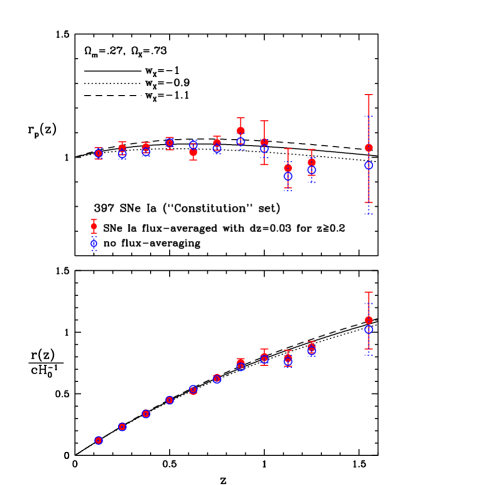
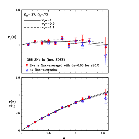
We have flux-averaged the SNe Ia at $z\geq 0.2$, to minimize any likely systematic biases due to lensing or unknown systematic effects. It is interesting to note that flux-averaging has a more significant effect on the “Constitution” set. This is as expected, since the “Constitution” set is less homogeneous than the nearby+SDSS+ESSENCE+SNLS+HST data set, which include 103 SNe Ia from SDSS at $0.04<z<0.42$ Kessler09 . Flux-averaging brings both data sets closer to the prediction of a flat universe dominated by a cosmological constant.

Table I lists the distances measured from the nearby+SDSS+ESSENCE+SNLS+HST data set of 288 SNe Ia, flux-averaged with $dz=0.03$ at $z\geq 0.2$. Table II gives the corresponding normalized covariance matrix. Note that the distances measured from SNe Ia, $r_{p}(z_{i})$ ($i=1,2,...,11$), are only moderately correlated. Since the measurements of $r_{p}(z_{i})$ ($i=1,2,...,11$), as given by Tables I and II, encode all the distance information from the nearby+SDSS+ESSENCE+SNLS+HST data set of 288 SNe Ia independent of a cosmological model, they can be used in place of the full data set following the prescription given in Sec.II.4.

Table 1: Distances measured from 288 SNe Ia with 68% C.L. upper and lower uncertainties.

	$z$	$\overline{r_{p}}^{data}(z)$	$\sigma(r_{p})\,\,\,\,\,$	$\sigma\left(r_{p}(z)\right)^{+}$	$\sigma\left(r_{p}(z)\right)^{-}$
0	0.0	1.0000	–	–	–
1	0.125	1.0044	0.0129	0.9919	1.0171
2	0.25	1.0523	0.0129	1.0396	1.0651
3	0.375	1.0292	0.0199	1.0095	1.0490
4	0.5	1.0638	0.0244	1.0397	1.0878
5	0.625	1.0311	0.0245	1.0067	1.0556
6	0.75	1.0895	0.0321	1.0575	1.1212
7	0.875	1.0160	0.0356	0.9807	1.0512
8	1.0	1.0629	0.0398	1.0234	1.1022
9	1.125	1.0725	0.0747	0.9996	1.1452
10	1.25	1.0557	0.0427	1.0136	1.0977
11	1.551	0.9682	0.1505	0.8203	1.1151

Table 2: Normalized covariance matrix of distances measured from 288 SNe Ia

	1	2	3	4	5	6	7	8	9	10	11
1	1.0000	0.2539	0.5219	0.2016	0.3354	0.2148	0.2030	0.1741	0.0873	0.1728	0.0349
2	0.2539	1.0000	0.1386	0.2120	0.1496	0.1483	0.1068	0.1192	0.0635	0.0971	0.0323
3	0.5219	0.1386	1.0000	0.1288	0.2575	0.1413	0.1421	0.1130	0.0656	0.1106	0.0350
4	0.2016	0.2120	0.1288	1.0000	$-$0.0694	0.1473	0.0235	0.0917	0.0280	0.0650	0.0117
5	0.3354	0.1496	0.2575	$-$0.0694	1.0000	0.1236	0.1273	0.0677	0.0537	0.0809	0.0234
6	0.2148	0.1483	0.1413	0.1473	0.1236	1.0000	$-$0.1503	0.1709	$-$0.0173	0.0521	$-$0.0163
7	0.2030	0.1068	0.1421	0.0235	0.1273	$-$0.1503	1.0000	$-$0.0877	0.0796	0.0609	0.0515
8	0.1741	0.1192	0.1130	0.0917	0.0677	0.1709	$-$0.0877	1.0000	0.0811	0.0299	$-$0.0129
9	0.0873	0.0635	0.0656	0.0280	0.0537	$-$0.0173	0.0796	0.0811	1.0000	0.1779	0.3163
10	0.1728	0.0971	0.1106	0.0650	0.0809	0.0521	0.0609	0.0299	0.1779	1.0000	$-$0.4585
11	0.0349	0.0323	0.0350	0.0117	0.0234	$-$0.0163	0.0515	$-$0.0129	0.3163	$-$0.4585	1.0000

III.2 Measurements of the Dark Energy Density Function and $H(z)$

The most transparent way to see how current data compare to the prediction of the cosmological constant model is to measure the dark energy density function. Fig.3-4 show the dark energy density function measured from combining SN Ia data with CMB, BAO, GRB data, and imposing the SHOES prior on $H_{0}$, for SNe Ia from the “Constitution” and the nearby+SDSS+ESSENCE+SNLS+HST data sets respectively, without assuming a flat universe. Fig.5 and Fig.6 are similar to Fig.3 and Fig.4, except a flat universe is assumed.

Figure 3: Dark energy density function $X(z)\equiv\rho_{X}(z)/\rho_{X}(0)$ measured from combining SN Ia data (the “Constitution” set of 397 SNe Ia) with CMB, BAO, GRB data, and imposing the SHOES prior on $H_{0}$. The 68% (shaded) and 95% confidence level regions are shown.

Figure 4: Dark energy density function $X(z)\equiv\rho_{X}(z)/\rho_{X}(0)$ measured from combining SN Ia data (nearby+SDSS+ESSENCE+SNLS+HST data set of 288 SNe Ia) with CMB, BAO, and GRB data, and imposing the SHOES prior on $H_{0}$. The 68% (shaded) and 95% confidence level regions are shown.

Figure 5: Dark energy density function $X(z)\equiv\rho_{X}(z)/\rho_{X}(0)$ measured from combining SN Ia data (the “Constitution” set of 397 SNe Ia) with CMB, BAO, GRB data, and imposing the SHOES prior on $H_{0}$. The 68% (shaded) and 95% confidence level regions are shown. A flat universe is assumed.

Figure 6: Dark energy density function $X(z)\equiv\rho_{X}(z)/\rho_{X}(0)$ measured from combining SN Ia data (nearby+SDSS+ESSENCE+SNLS+HST data set of 288 SNe Ia) with CMB, BAO, and GRB data, and imposing the SHOES prior on $H_{0}$. The 68% (shaded) and 95% confidence level regions are shown. A flat universe is assumed. (a) Assuming $X(z\geq 1)=X(z=1)$. (b) Same as (a), but with $X(z=1.5)$ added as a parameter, and assuming $X(z\geq 1.5)=X(z=1.5)$.

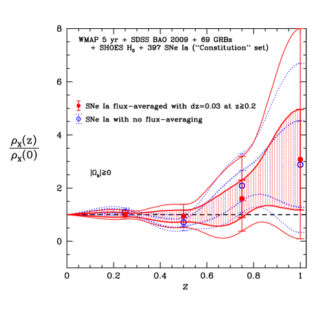
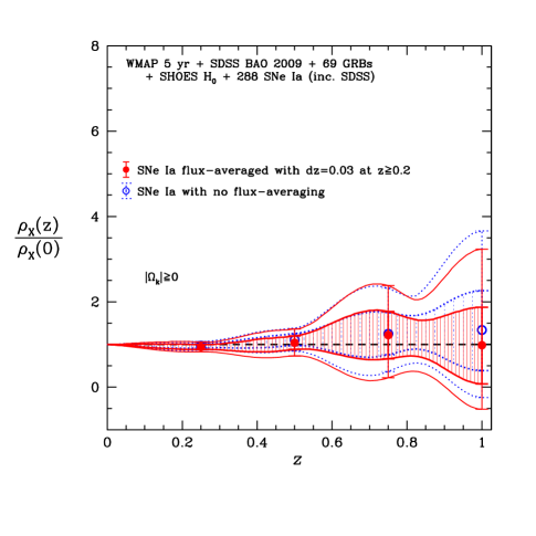
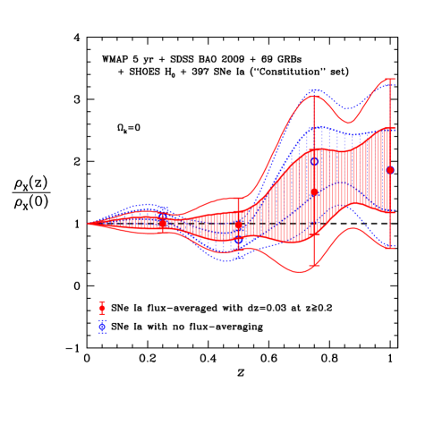
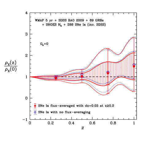
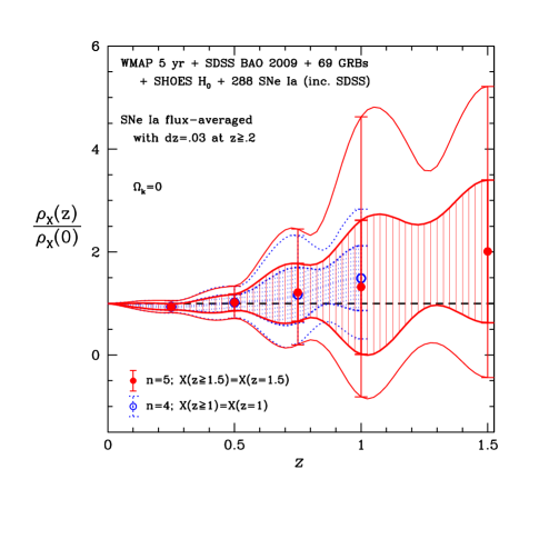
Again, the same trend as in Figs.1-2 is seen: using the nearby+SDSS+ESSENCE+SNLS+HST data set of SNe Ia gives much more stringent constraints on dark energy than using the “Constitution” set of SNe Ia, and gives measurements that are closer to a cosmological constant. Flux-averaging again has larger impact on the results from using the “Constitution” set of SNe Ia, and brings the measurements closer to that predicted by a cosmological constant.

Note that the $X(z)$ measured using the “Constitution” set of SNe Ia actually deviates from a cosmological constant at $\sim$2$\sigma$ without flux-averaging; the downturn in the measured $X(z)$ at $z\sim 0.25-0.5$ is consistent with that found by Huang et al. (2009) Huang09 . Since this apparent variation in $X(z)$ disappears in the results from using the nearby+SDSS+ESSENCE+SNLS+HST set of SNe Ia without flux-averaging, it is likely that it originated from unknown systematic effects in the “Constitution” set of SNe Ia.

Fig.6(a) shows that assuming a flat universe, dark energy is detected at $>2\sigma$ at $z=1$ using the nearby+SDSS+ESSENCE+SNLS+HST data set of 288 SNe Ia, together with CMB, BAO, and GRB data. Fig.6(b) is the same as Fig.6(a), but with $X(z=1.5)$ added as a parameter, and assuming $X(z\geq 1.5)=X(z=1.5)$. The $X(z)$ results at $z\leq 0.75$ remain about the same, while the errors for $X(z=1)$ are larger (but the mean value of $X(z)$ remains about the same) because of the additional parameter allowed. Independent of the assumptions about $X(z)$ at $z\geq 1$, dark energy is detected at $>98$% confidence level for $z\leq 0.75$.

Figure 7: The measured cosmic expansion history $H(z)$ corresponding to Fig.3. The error bars represent the 68% confidence level.

Figure 8: The measured cosmic expansion history $H(z)$ corresponding to Fig.4. The error bars represent the 68% confidence level.

Figs.7-8 are the measurements of the cosmic expansion history $H(z)$ that correspond to Fig.3-4.

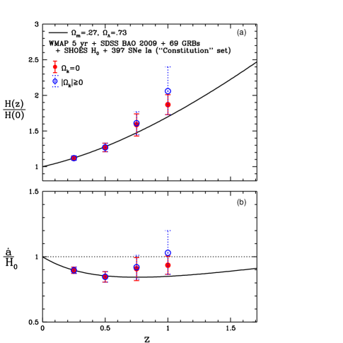
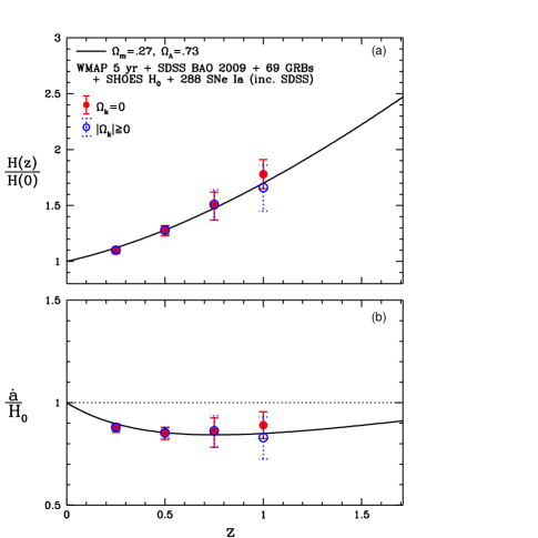
Table III gives the dark energy density function $X(z)\equiv\rho_{X}(z)/\rho_{X}(0)$ and the cosmic expansion history $H(z)$ measured from current data (nearby+SDSS+ESSENCE+SNLS+HST data set of 288 SNe Ia, together with CMB, BAO, GRB data, and imposing the SHOES prior on $H_{0}$). The $H(z)$ measurements are derived using Eq.(II). Tables IV and V give the normalized covariance matrices of the $X(z)$ and $H(z)$ measurements. Note that both the $X(z)$ and $H(z)$ measurements are only weakly correlated.

Table 3: $X(z)$, $H(z)$, and cosmological parameters estimated from current data with 68% C.L. upper and lower uncertainties.

	$\mu$	$\sigma$	$\sigma^{-}$	$\sigma^{+}$
$X(z=0.2)$	0.942	0.059	0.884	1.001
$X(z=0.5)$	1.041	0.159	0.883	1.199
$X(z=0.75)$	1.223	0.556	0.667	1.776
$X(z=1.0)$	0.987	0.960	0.089	1.869
$\Omega_{m}$	0.262	0.016	0.246	0.278
$\Omega_{k}$	$-$0.009	0.012	$-$0.020	0.003
$h$	0.709	0.020	0.690	0.729
$\omega_{b}$	0.02377	0.00062	0.02321	0.02441
$H(z=0.25)$	1.10	0.021	1.08	1.12
$H(z=0.5)$	1.28	0.043	1.24	1.32
$H(z=0.75)$	1.51	0.132	1.37	1.64
$H(z=1.0)$	1.66	0.215	1.45	1.86

Table 4: Normalized covariance matrix of $X(z)$ from current data

	1	2	3	4
1	1.0000	$-$0.1273	$-$0.0668	0.0078
2	$-$0.1273	1.0000	$-$0.0374	$-$0.2789
3	$-$0.0668	$-$0.0374	1.0000	$-$0.3638
4	0.0078	$-$0.2789	$-$0.3638	1.0000

Table 5: Normalized covariance matrix of $H(z)$ from current data

	1	2	3	4
1	1.0000	$-$0.1665	$-$0.1212	0.1493
2	$-$0.1665	1.0000	$-$0.1524	$-$0.2281
3	$-$0.1212	$-$0.1524	1.0000	$-$0.3605
4	0.1493	$-$0.2281	$-$0.3605	1.0000

III.3 Constraints on ($w_{0},w_{a})$, ($w_{0},w_{0.5}$)

For comparison with the work of others, Figs.9-10 show the 68% and 95% joint confidence level contours of ($w_{0},w_{a})$ and ($w_{0},w_{0.5}$), from combining SN Ia data with CMB, BAO, GRB data, and imposing the SHOES prior on $H_{0}$, for SNe Ia from the “Constitution” and the nearby+SDSS+ESSENCE+SNLS+HST data sets respectively,

Figure 9: The 68% and 95% joint confidence level contours on constraints on ($w_{0},w_{a})$ and ($w0,w_{0.5}$), using SN Ia data (the “Constitution” set of 397 SNe Ia) together with CMB, BAO, GRB data, and imposing the SHOES prior on $H_{0}$.

Figure 10: The 68% and 95% joint confidence level contours on constraints on ($w_{0},w_{a})$ and ($w0,w_{0.5}$), using SN Ia data (the nearby+SDSS+ESSENCE+SNLS+HST set of 288 SNe Ia) together with CMB, BAO, GRB data, and imposing the SHOES prior on $H_{0}$.

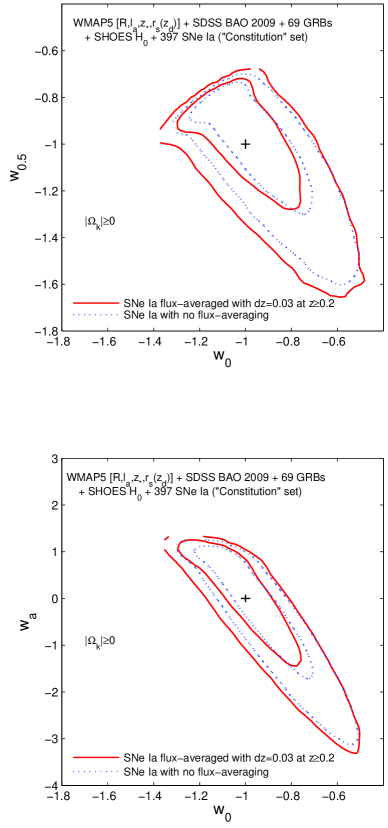
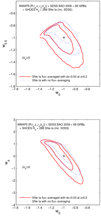
It is interesting to note that flux-averaging has a larger impact on the ($w_{0},w_{a})$ and ($w_{0},w_{0.5}$) error contours from the combined data using the nearby+SDSS+ESSENCE+SNLS+HST set of SNe Ia, compared to the combined data using the “Constitution” of SNe Ia. This is in contrast to what we found when measuring the dark energy density function $X(z)$ at $z=0.25,0.5,0.75,1$ (see Figs.3-4). A comparison of the correlation coefficients in Tables IV and VI reveal that assuming a linear dark energy equation-of-state results in much stronger correlations among the dark energy parameters. This obsures some of the information about dark energy contained in the data.

III.4 Dark Energy Figure of Merit from Current Data

Wang (2008a) Wang08a defined a general dark energy Figure-of-Merit (FoM)

$${\rm FoM}=\frac{1}{\sqrt{{\rm detCov}(f_{1},f_{2},...f_{N})}}$$ (23)

where $(f_{1},f_{2},...f_{N})$ is the set of parameters that have been chosen to parametrize dark energy.

The Dark Energy Task Force (DETF) defined the dark energy FoM to be the inverse of the area enclosed by the 95% confidence level contour of $(w_{0},w_{a})$ deft (2006). The areas enclosed by contours are difficult to calculate for real data, as these contours can be quite irregular (see Figs.9-10). The definition of Eq.(23) has the advantage of being easy to calculate for either real or simulated data. For $(f_{1},f_{2})=(w_{0},w_{a})$, ${\rm FoM}$ of Eq.(23) is proportional to the FoM defined by the DETF for ideal Gaussian-distributed data, and the same as the relative FoM used by the DETF in Fisher matrix forecasts.

Table VI shows the dark energy FoM from SN Ia data together with CMB, BAO, GRB data, and imposing the SHOES prior on $H_{0}$, for the dark energy density function $X(z)\equiv\rho_{X}(z)/\rho_{X}(0)$ measured at $z=0.25,0.5,0.75,1.0$ (with X(z) given by cubic spline elsewhere and assuming $X(z>1)=X(1)$, see Sec.II.5) and a dark energy equation-of-state linear in $a$ parametrized by ($w_{0},w_{0.5}$) and ($w_{0},w_{a}$) respectively.

Table 6: Dark energy FoM from current data

data: CMB+BAO+GRB+	FoM${}_{r}(\{X_{i}\})$	$\sigma(w_{0})$	$\sigma(w_{0.5})$	$r_{w_{0},w_{0.5}}$	FoM${}_{r}(w_{0},w_{0.5})$	$\sigma(w_{0})$	$\sigma(w_{a})$	$r_{w_{0},w_{a}}$	FoM${}_{r}(w_{0},w_{a})$
288 SNe Ia (inc. SDSS)	230.7	0.1473	0.1688	$-$0.6676	54.0	0.1475	0.8708	$-$0.9029	18.1
397 SNe Ia (“Constitution”)	44.1	0.1841	0.2252	$-$0.7530	36.6	0.1845	1.1349	$-$0.9232	12.4

It is interesting to note that for $\{X(z_{i})\}$ ($z_{i}$=0.25, 0.5, 0.75, 1.0), the factor of improvement in the dark energy FoM is 5.2 when the nearby+SDSS+ESSENCE+SNLS+HST data set of 288 SNe Ia is used instead of the “Constitution” set of 397 SNe Ia (see Table VI); this quantifies the difference between Fig.4 and Fig.3. For a linear dark energy equation of state, the improvement in FoM is a little less than $\sim$50% (see Table VI). The same equation of state linear in $a$ can be written in either ($w_{0},w_{0.5}$) or ($w_{0},w_{a}$) (see Sec.II.5). As expected, the parameters ($w_{0},w_{0.5}$) are significantly less correlated than ($w_{0},w_{a}$) Wang08a , thus represent a better choice of parameters. The improvement in the dark energy FoM is slightly larger for ($w_{0},w_{0.5}$) than for ($w_{0},w_{a}$).

III.5 The Impact of Adding CMB Constraints on $r_{s}(z_{d})$

Compared to previous work using CMB distances priors, we have added the constraints on $r_{s}(z_{d})$. Not surprisingly, this has negligible impact on $X(z)$ measured from current data, since we have assumed that $X(z>1)=X(z=1)$.

Figs.11-12 show the difference in the marginalized probability density distributions of the dark energy and cosmological parameters using [$R(z_{*}),l_{a}(z_{*}),z_{*},r_{s}(z_{d})]$ (as we have done throughout this paper), and using [$R(z_{*}),l_{a}(z_{*}),\omega_{b}$]. Clearly, adding CMB constraints on $r_{s}(z_{d})$ tightens the constraints on ($w_{0},w_{a})$ and ($w_{0},w_{0.5}$), as these are parameters from assuming a dark energy equation-of-state linear in the cosmic scale factor $a$, thus imply strong assumptions about early dark energy that are propagated to the low and intermediate redshifts Wang & Tegmark (2004).

We find that the constraints on [$R(z_{*}),l_{a}(z_{*}),z_{*},r_{s}(z_{d})]$ summarize all useful information from CMB data that are relevant to dark energy and are geometric and independent of dark energy perturbations. Further adding constraints on $z_{d}$ does not add new information, since $z_{d}$ is well approximated by Eq.(10), which only depends on $\Omega_{m}h^{2}$ and $\Omega_{b}h^{2}$, and which in turn are already constrained by [$R(z_{*}),l_{a}(z_{*}),z_{*},r_{s}(z_{d})]$.

Figure 11: Marginalized probability distributions of the dark energy and cosmological parameters using SN Ia data (the nearby+SDSS+ESSENCE+SNLS+HST set of 288 SNe Ia flux-averaged at $z\geq 0.2$) together with CMB, BAO, GRB data, and imposing the SHOES prior on $H_{0}$, assuming a linear dark energy equation of state parametrized by ($w_{0},w_{0.5}$) (see Eq.[20]). The solid and dashed lines indicate the use of the CMB data summarized by [$R(z_{*}),l_{a}(z_{*}),z_{*},r_{s}(z_{d})]$, and [$R(z_{*}),l_{a}(z_{*}),\omega_{b}$] respectively.

Figure 12: Same as Fig.11, except the linear dark energy equation of state is parametrized by the usual ($w_{0},w_{a}$).

IV Summary and Discussion

It is likely that current sets of SNe Ia may be contaminated by unknown systematic effects Qi09 ; Sanchez09 . We have used the flux-averaging of SNe Ia (which was developed to reduce the weak lensing systematic effect Wang (2000b); Wang & Mukherjee (2004); Wang (2005)) to help reduce the impact of unknown systematic effects. Since the SNe Ia in each redshift bin are flux-averaged and not used directly in the likelihood analysis, the systematic bias that results from unknown systematic errors from individual SNe Ia can be minimized. For homogeneous data without unknown systematic errors, flux-averaging should not change the results qualitatively at intermediate redshifts (where the lensing effect is negligible). Thus in addition to reducing lensing and lensing-like systematic effects, flux-averaging of SN Ia data provide a useful test for the presence of unknown systematic effects at intermediate redshifts.

We find that flux-averaging has a significantly smaller effect on the nearby+SDSS+ESSENCE+SNLS+HST data set of 288 SNe Ia Kessler09 , compared to the “Constitution” set of 397 SNe Ia Hicken09 , see Figs.1 and 2. This same trend continues when the SN Ia data are combined with CMB, BAO, GRB data, and the SHOES measurement of $H_{0}$ to measure the dark energy density function, see Figs.3-6. Furthermore, flux-averaging brings both data sets closer to the predictions of a flat universe dominated by a cosmological constant (see Figs.1-8). The nearby+SDSS+ESSENCE+SNLS+HST data set of SNe Ia (together with CMB, BAO, GRB data, and the SHOES measurement of $H_{0}$) are consistent with a cosmological constant at 68% confidence level with or without flux-averaging of SNe Ia (see Fig.4). Without flux-averaging, the combined data using the “Constitution” set of 397 SNe Ia seem to indicate a deviation from a cosmological constant at $\sim$95% confidence at $0\mathrel{\mathchoice{\lower 3.6pt\vbox{\halign{$\mathsurround=0pt\displaystyle\hfill#\hfil$\cr<\crcr\sim\crcr}}}{\lower 3.6pt\vbox{\halign{$\mathsurround=0pt\textstyle\hfill#\hfil$\cr<\crcr\sim\crcr}}}{\lower 3.6pt\vbox{\halign{$\mathsurround=0pt\scriptstyle\hfill#\hfil$\cr<\crcr\sim\crcr}}}{\lower 3.6pt\vbox{\halign{$\mathsurround=0pt\scriptscriptstyle\hfill#\hfil$\cr<\crcr\sim\crcr}}}}z\mathrel{\mathchoice{\lower 3.6pt\vbox{\halign{$\mathsurround=0pt\displaystyle\hfill#\hfil$\cr<\crcr\sim\crcr}}}{\lower 3.6pt\vbox{\halign{$\mathsurround=0pt\textstyle\hfill#\hfil$\cr<\crcr\sim\crcr}}}{\lower 3.6pt\vbox{\halign{$\mathsurround=0pt\scriptstyle\hfill#\hfil$\cr<\crcr\sim\crcr}}}{\lower 3.6pt\vbox{\halign{$\mathsurround=0pt\scriptscriptstyle\hfill#\hfil$\cr<\crcr\sim\crcr}}}}0.8$, but is consistent with a cosmological constant at $\sim$68% confidence when SNe Ia are flux-averaged (see Fig.3).

It is interesting to note that for a dark energy density function $X(z)$ parametrized by $\{X(z_{i})\}$ ($z_{i}$=0.25, 0.5, 0.75, 1.0) and assumed to be constant at $z>1$, the factor of improvement in the dark energy FoM is 5.2 when the nearby+SDSS+ESSENCE+SNLS+HST data set of 288 SNe Ia is used instead of the “Constitution” set of 397 SNe Ia (see Table VI). For a linear dark energy equation of state, the improvement in FoM is a little less than $\sim$50%. This indicates that current data already contain more information about dark energy than can be adequately represented by a linear dark energy equation of state. Using the nearby+SDSS+ESSENCE+SNLS+HST data set of 288 SNe Ia gives more stringent constraints on dark energy than using the “Constitution” set of 397 SNe Ia, because the former data set includes 103 SNe Ia from SDSS at $0.04<z<0.42$ Kessler09 which are not in the latter data set, and because the latter data set is less homogeneous and likely more prone to unknown systematic effects.

We have measured the dark energy density function $X(z)$ from data without imposing $X(z)\geq 0$. Since the probability density distributions for $X(z)$ that we have obtained from the current data extend to $X(z)<0$, it is not possible to convert the measurements of $X(z)$ into measurements of $w_{X}(z)=p_{X}(z)/\rho_{X}(z)$, or the deceleration parameter $q(z)$ (which depends on $w_{X}(z)$). $X(z)$ is related to the dark energy equation of state $w_{X}(z)$ as follows Wang & Garnavich (2001):

$$X(z)\equiv\frac{\rho_{X}(z)}{\rho_{X}(0)}=\exp\left\{\int_{0}^{z}{\rm d}z^{\prime}\,\frac{3[1+w_{X}(z^{\prime})]}{1+z^{\prime}}\right\}.$$ (24)

Hence parametrizing dark energy with $w_{X}(z)$ implicitly assumes that $\rho_{X}(z)$ does not change sign in cosmic time (i.e., $X(z)\geq 0$). This precludes whole classes of dark energy models in which $\rho_{X}(z)$ becomes negative in the future (“Big Crunch” models, see Refs.Linde (1987); WangLinde04 for an example) Wang & Tegmark (2004). Thus the measurement of $X(z)$, without assuming $X(z)\geq 0$, contains more information about dark energy than that of $w_{X}(z)$ or $q(z)$.

Our work complements Genovese et al. (2009) Genovese09 , and Bogdanos & Nesseris (2009) Bogdanos09 , both of these papers assumed a flat universe, and analyzed SN Ia data only. Genovese et al. (2009) used model-testing (see e.g. Liddle06 ) to diffentiate assumptions about $w_{X}(z)$, and derived parametric and non-parametric estimators of $w_{X}(z)$ Genovese09 . Bogdanos & Nesseris (2009) used genetic algorithms to derive model-independent constraints on the distance modulus from SNe Ia, which are then used to constrain $w_{X}(z)$ Bogdanos09 . In this paper, we have derived model-independent constraints on $X(z)$, instead of $w_{X}(z)$, for both a flat universe and a universe with arbitrary spatial curvature. We also use newer SN Ia data (which significantly tighten the dark energy constraints), and combine with CMB, BAO, GRB data, and the SHOES measurement of $H_{0}$.

Finally, we note that the ($w_{0},w_{a}$) FoM for current data (the nearby+SDSS+ESSENCE+SNLS+HST data set of 288 SNe Ia flux-averaged, with CMB, BAO, GRB data, and the SHOES prior on $H_{0}$) is 18.1, more than a factor of two larger than that found by Wang (2008a) using data available in March 2008 (182 SNe Ia compiled by Riess et al. 2007 Riess (2007), $[R(z_{*}),l_{a}(z_{*}),\Omega_{b}h^{2}]$ from the five year WMAP observations, the SDSS measurement of the BAO scale by Eisenstein et al. 2005 Eisenstein et al. (2005), and assuming the HST prior of $H_{0}=72\pm 8\,$km s^-1Mpc^-1). Most of this gain results from the significantly improved distance measurements from SNe Ia (see Figs.1-2). Assuming a flat universe, dark energy is detected at $>98$% confidence level for $z\leq 0.75$ using the combined data with 288 SNe Ia from nearby+SDSS+ESSENCE+SNLS+HST, independent of the assumptions about $X(z\geq 1)$ (see Fig.6).

In order to make solid progress on probing dark energy, it will be essential to launch aggressive observational projects to obtain large and uniform sets of SNe Ia spanning the redshift range of $0\mathrel{\mathchoice{\lower 3.6pt\vbox{\halign{$\mathsurround=0pt\displaystyle\hfill#\hfil$\cr<\crcr\sim\crcr}}}{\lower 3.6pt\vbox{\halign{$\mathsurround=0pt\textstyle\hfill#\hfil$\cr<\crcr\sim\crcr}}}{\lower 3.6pt\vbox{\halign{$\mathsurround=0pt\scriptstyle\hfill#\hfil$\cr<\crcr\sim\crcr}}}{\lower 3.6pt\vbox{\halign{$\mathsurround=0pt\scriptscriptstyle\hfill#\hfil$\cr<\crcr\sim\crcr}}}}z\mathrel{\mathchoice{\lower 3.6pt\vbox{\halign{$\mathsurround=0pt\displaystyle\hfill#\hfil$\cr<\crcr\sim\crcr}}}{\lower 3.6pt\vbox{\halign{$\mathsurround=0pt\textstyle\hfill#\hfil$\cr<\crcr\sim\crcr}}}{\lower 3.6pt\vbox{\halign{$\mathsurround=0pt\scriptstyle\hfill#\hfil$\cr<\crcr\sim\crcr}}}{\lower 3.6pt\vbox{\halign{$\mathsurround=0pt\scriptscriptstyle\hfill#\hfil$\cr<\crcr\sim\crcr}}}}2$ Wang (2000a).

Acknowledgements I am grateful to Eiichiro Komatsu for helpful comments and for making the covariance matrix for [$R(z_{*}),l_{a}(z_{*}),\Omega_{b}h^{2},r_{s}(z_{d})$] from WMAP 5 year data available, and I acknowledge the use of cosmomc in processing the MCMC chains.

References

- Riess et al. (1998) Riess, A. G, et al., 1998, Astron. J., 116, 1009
- Perlmutter et al. (1999) Perlmutter, S. et al., 1999, ApJ, 517, 565
- Komatsu et al. (2009) Komatsu, E., et al. 2009, Astrophys.J.Suppl., 180, 330
- (4) Sollerman, J., et al., Astrophysical Journal 703 (2009) 1374
- (5) Serra, P., et al., arXiv:0908.3186
- (6) Reid, B.A., et al., arXiv:0907.1659
- (7) Biswas, R., Wandelt, B.D., arXiv:0903.2532
- (8) Daly, R.A., et al., ApJ, 691, 1058 (2009)
- (9) Samushia, L., et al., arXiv:0906.2734
- (10) Shafieloo, A., Sahni, V., Starobinsky, A.A., arXiv:0903.5141
- Freese et al. (1987) Freese, K., Adams, F.C., Frieman, J.A., and Mottola, E., Nucl. Phys. B287, 797 (1987).
- Linde (1987) Linde A D, “Inflation And Quantum Cosmology,” in Three hundred years of gravitation, (Eds.: Hawking, S.W. and Israel, W., Cambridge Univ. Press, 1987), 604-630.
- Peebles & Ratra (1988) Peebles, P.J.E., and Ratra, B., 1988, ApJ, 325, L17
- Wetterich (1988) Wetterich, C., 1988, Nucl.Phys., B302, 668
- Frieman et al. (1995) Frieman, J.A., Hill, C.T., Stebbins, A., and Waga, I., 1995, PRL, 75, 2077
- Caldwell, Dave & Steinhardt (1998) Caldwell, R., Dave, R., & Steinhardt, P.J., 1998, PRL, 80, 1582
- (17) Kaloper, N., & Sorbo, L., JCAP 0604 (2006) 007
- (18) Chiba, T.; Dutta, S., & Scherrer, R.J., Phys.Rev.D80:043517,2009
- Sahni & Habib (1998) Sahni, V., & Habib, S., 1998, PRL, 81, 1766
- Parker & Raval (1999) Parker, L., and Raval, A., 1999, PRD, 60, 063512
- Boisseau et al. (2000) Boisseau, B., Esposito-Farèse, G., Polarski, D. & Starobinsky, A. A. 2000, Phys. Rev. Lett., 85, 2236
- Dvali, Gabadadze, & Porrati (2000) Dvali, G., Gabadadze, G., & Porrati, M. 2000, Phys.Lett. B485, 208
- Freese & Lewis (2002) Freese, K., & Lewis, M., 2002, Phys. Lett. B, 540, 1
- (24) Padmanabhan, T., arXiv:0807.2356
- (25) Kahya, E. O.; Onemli, V. K.; Woodard, R. P., arXiv:0904.4811
- (26) O’Callaghan, E., Gregory, R., Pourtsidou, A., JCAP 0909:020,2009
- (27) Copeland, E. J., Sami, M., Tsujikawa, S., IJMPD, 15 (2006), 1753
- (28) Ruiz-Lapuente, P., Class. Quantum. Grav., 24 (2007), 91
- (29) Ratra, B., Vogeley, M. S., arXiv:0706.1565 (2007)
- (30) Frieman, J., Turner, M., Huterer, D., ARAA, 46, 385 (2008)
- (31) Caldwell, R. R., & Kamionkowski, M., arXiv:0903.0866
- (32) Uzan, J.-P., arXiv:0908.2243
- (33) Cimatti, A., et al., Experimental Astronomy, 23, 39 (2009)
- (34) Refregier, A., et a., Exper.Astron.23:17-37,2009
- (35) Hicken, M., et al. 2009, ApJ, 700, 1097
- (36) Kessler, R., et al. 2009, arXiv0908.4274
- Guy et al. (2005) Guy, J.; Astier, P.; Nobili, S.; Regnault, N.; Pain, R., 2005, A&A,443, 781
- Guy et al. (2007) Guy, J., et al. 2007, A&A, 466, 11
- Phillips (1993) Phillips, M. M. 1993, ApJ, 413, L105
- Riess, Press, & Kirshner (1995) Riess, A.G., Press, W.H., & Kirshner, R.P., ApJ, 438, L17 (1995)
- Jha, Riess, & Kirshner (2007) Jha, S.; Riess, A.G.; Kirshner, R.P. 2007, ApJ, 659, 122
- (42) Qi, S.; Lu, T.; & Wang, F.-Y., MNRAS, 398 (2009) L78-L82
- (43) Bueno Sanchez, J.C.; Nesseris, S., & Perivolaropoulos, L., arXiv:0908.2636
- Wang (2000b) Wang, Y., ApJ 536, 531 (2000b)
- Wang & Mukherjee (2004) Wang, Y., & Mukherjee, P. 2004, ApJ, 606, 654
- Wang (2005) Wang, Y., JCAP, 03, 005 (2005), astro-ph/0406635
- Wang & Mukherjee (2007) Wang, Y., & Mukherjee, P., PRD, 76, 103533 (2007)
- Page (2003) Page, L., et al. 2003, ApJS, 148, 233
- (49) Komatsu, E., “wmap-prior-for-bao.pdf” at http://gyudon.as.utexas.edu/komatsu/wmap5/
- (50) Wang, Y., 2008a, Phys. Rev. D 77, 123525
- Hu & Sugiyama (1996) Hu, W., & Sugiyama, N. 1996, ApJ, 471, 542
- Eisenstein & Hu (1998) Eisenstein, D. & Hu, W. 1998, ApJ, 496, 605
- (53) Percival, W.J., et al. 2009, arXiv0907.1660
- (54) Wang, Y., 2008b, PRD, 78, 123532
- (55) Schaefer, B. E., 2007, ApJ, 660, 16
- Wang & Garnavich (2001) Wang, Y., and Garnavich, P. 2001, ApJ, 552, 445
- Wang & Tegmark (2004) Wang, Y., & Tegmark, M. 2004, Phys. Rev. Lett., 92, 241302
- Wang & Freese (2006) Wang, Y., & Freese, K. 2006, Phys.Lett. B632, 449 (astro-ph/0402208)
- Chev01 (2001) Chevallier, M., & Polarski, D. 2001, Int. J. Mod. Phys. D10, 213
- Lewis02 (2002) Lewis, A., & Bridle, S. 2002, PRD, 66, 103511
- (61) Riess, A.G. , et al. 2009, ApJ, 699, 539
- (62) Huang, Q.-G., Li, M.; Li, X.-D.; Wang, S., arXiv:0905.0797
- deft (2006) Albrecht, A.; Bernstein, G.; Cahn, R.; Freedman, W. L.; Hewitt, J.; Hu, W.; Huth, J.; Kamionkowski, M.; Kolb, E.W.; Knox, L.; Mather, J.C.; Staggs, S.; Suntzeff, N.B., Report of the Dark Energy Task Force, astro-ph/0609591
- (64) Wang, Y.; Kratochvil, J. M.; Linde, A.; & Shmakova, M., JCAP 0412 (2004) 006
- (65) Genovese, C., et al., Annals of Applied Statistics 2009, Vol. 3, No. 1, 144
- (66) Bogdanos, C., & Nesseris, S., JCAP05(2009)006
- (67) Liddle, A.R.; Mukherjee, P.; Parkinson, D.; & Wang, Y., Phys.Rev.D74 (2006) 123506
- Riess (2007) Riess, A.G., et al., astro-ph/0611572
- Eisenstein et al. (2005) Eisenstein, D., et al., ApJ, 633, 560
- Wang (2000a) Wang, Y., ApJ 531, 676 (2000a)