Symmetries and exponential error reduction in YM theories on the lattice: theoretical aspects and simulation results

Abstract:

The path integral of a quantum system with an exact symmetry can be written as a sum of functional integrals each giving the contribution from quantum states with definite symmetry properties. We propose a strategy to compute each of them, normalized to the one with vacuum quantum numbers, by a Monte Carlo procedure whose cost increases power-like with the time extent of the lattice. This is achieved thanks to a multi-level integration scheme, inspired by the transfer matrix formalism, which exploits the symmetry and the locality in time of the underlying statistical system. As a result the cost of computing the lowest energy level in a given channel, its multiplicity and its matrix elements is exponentially reduced with respect to the standard path-integral Monte Carlo. We briefly illustrate the approach in the simple case of the one-dimensional harmonic oscillator and discuss in some detail its extension to the four-dimensional Yang Mills theories. We report on our recent new results in the SU(3) Yang–Mills theory on the relative contribution to the partition function of the parity-odd states.

MKPH-T-09-20

CERN-PH-TH/2009-189

1 Introduction

1.1 The problem

Lattice field theories can be studied numerically by Monte Carlo simulations. They allow to address non-perturbative problems from first principles, and for most of the theories the lattice provides the only known non-perturbative definition. The mass of the lowest states in a given channel can, for instance, be extracted from the Euclidean time-dependence of a suitable two-point correlation function. Very often, however, the statistical error of the Monte Carlo estimate grows exponentially with time, and in practice it is not possible to find a window where statistical and systematic errors are both under control. The problem is easily explained by looking at the states contributing asymptotically in time to the two-point function and to its variance. Whenever the energy of the asymptotic state in the variance is smaller than twice that in the two-point function, the noise to signal ratio is going to grow exponentially in time [1, 2]. The standard Monte Carlo approach fails basically because for any given field configuration all asymptotic states of the theory are allowed to propagate in the time direction, regardless of the quantum numbers of the source fields. Their contributions disappear in the Monte Carlo average for the two-point function but sum up in the noise. As shown in the following subsection, the issue is already there for a simple system such as the harmonic oscillator. We use the latter to introduce the basic ideas of the method that was proposed in [3, 4], a “symmetry-constrained” Monte Carlo, and to show how it avoids the exponential increase of the signal-to-noise ratio.

1.2 The case of the harmonic oscillator

We consider the one-dimensional harmonic oscillator on the lattice. We recall here a few basic equations. More details can be found in [3] to which we refer for any unexplained notation. The system is described by the Hamiltonian

$$\hat{H}=\frac{\hat{p}^{2}}{2m}+V(\hat{x})\quad{\rm with}\quad V(\hat{x})=\frac{1}{2}m\omega^{2}\hat{x}^{2}\;.$$ (1)

This operator is invariant under parity transformations, therefore its eigenstates can be classified according to a parity quantum number ($+$ or $-$). We label the corresponding energy levels as ${\cal E}_{i}^{+}$ and ${\cal E}_{j}^{-}$ respectively. The transfer operator between two consecutive time slices is defined as

$$\hat{\cal T}=e^{-\frac{a}{2}V(\hat{x})}\,e^{-a\frac{\hat{p}^{2}}{2m}}\,e^{-\frac{a}{2}V(\hat{x})}\;,$$ (2)

an its matrix elements in the coordinate basis

$$\langle x_{n+1}|\hat{\cal T}|x_{n}\rangle\equiv\left(\frac{m}{2\pi a}\right)^{1/2}T_{n+1,n}$$ (3)

can be computed explicitly

$$T_{n+1,n}=e^{-aL_{n+1,n}}\;,$$ (4)

with

$$L_{n+1,n}\equiv{\cal L}(x_{n+1},x_{n})=\frac{m}{2}\left(\frac{x_{n+1}-x_{n}}{a}\right)^{2}+\frac{V(x_{n+1})}{2}+\frac{V(x_{n})}{2}\;.$$ (5)

The statistical variance associated to the two-point correlation function $\langle x_{l}x_{k}\rangle$ (interpolating parity odd states) is

$$\sigma^{2}=\langle x^{2}_{l}x^{2}_{k}\rangle-\langle x_{l}x_{k}\rangle^{2}\;,$$ (6)

and, at asymptotically large time separations, the signal-to-noise ratio can be easily computed in the underlying quantum field theory

$$\frac{\langle x_{l}x_{k}\rangle}{\sigma}=\frac{|\langle{\cal E}_{0}^{-}|\hat{x}|{\cal E}_{0}^{+}\rangle|^{2}}{|\langle{\cal E}_{0}^{+}|\hat{x}^{2}|{\cal E}_{0}^{+}\rangle|}\,e^{-a\,({\cal E}_{0}^{-}-{\cal E}_{0}^{+})|l-k|}+\cdots$$ (7)

The ratio decreases exponentially in time, as announced. As we will describe in the following the problem here can be solved by introducing the “sign” and the “module” fields.

We define the complete set of parity eigenstates

$$|x,\pm\rangle=\frac{1}{\sqrt{2}}(|x\rangle\pm|-x\rangle)\;,\qquad\hat{\cal P}|x,\pm\rangle=\pm|x,\pm\rangle\;.$$ (8)

The invariance of the Hamiltonian under parity implies

$$\langle s^{\prime},x_{n+1}|\hat{\cal T}|x_{n},s\rangle=\left(\frac{2m}{\pi a}\right)^{1/2}T^{s}_{n+1,n}\,\delta_{s^{\prime}s}\;,$$ (9)

with

$$T^{s}_{n+1,n} = \frac{1}{2}\,e^{-a\Lambda^{+}_{n+1,n}}\left\{e^{a\Lambda^{-}_{n+1,n}}+s\,e^{-a\Lambda^{-}_{n+1,n}}\right\}\;,$$ (10)

$$\Lambda^{\pm}_{n+1,n} = \frac{1}{2}\Big{\{}{\cal L}(-x_{n+1},x_{n})\pm{\cal L}(x_{n+1},x_{n})\Big{\}}\;,$$ (11)

and the functional integral can be written as

$$Z=\sum_{s=\pm}Z^{s}\;,\qquad Z^{s}=\int\prod_{n=0}^{N-1}dx_{n}\,T^{s}_{n+1,n}\;,$$ (12)

where $N$ is the extent of the lattice. We further define

$$T^{+}_{n+1,n}\equiv e^{-aL^{+}_{n+1,n}}=e^{-a\Lambda^{+}_{n+1,n}}\cosh\{\,a\Lambda^{-}_{n+1,n}\}\;,$$ (13)

and cast the functional integrals in the form

$$Z^{+}=\int\prod_{n=0}^{N-1}dx_{n}\,e^{-S^{+}}\;,\qquad Z^{-}=\int\prod_{n=0}^{N-1}dx_{n}\,e^{-S^{+}}\prod_{m=0}^{N-1}\tanh\{a\,\Lambda^{-}_{m+1,m}\}\;,$$ (14)

where $S^{+}\equiv a\sum_{n=0}^{N-1}L^{+}_{n+1,n}$. The path integral is thus rewritten as a sum of two functional integrals giving the contribution from parity even and odd states respectively. Each integrand is a product of transfer matrix elements between quantum states with definite parity. The two-point correlation function reads ($k<l$)

$$\langle x_{l}x_{k}\rangle = \frac{1}{Z}\int\prod_{n=0}^{N-1}dx_{n}\,e^{-S^{+}}\Big{\{}x_{l}\prod_{m=k}^{l-1}\tanh\{a\,\Lambda^{-}_{m+1,m}\}x_{k}$$ (15)

$$+ \prod_{m=l}^{N-1}\tanh\{a\,\Lambda^{-}_{m+1,m}\}x_{l}x_{k}\prod_{m=0}^{k-1}\tanh\{a\,\Lambda^{-}_{m+1,m}\}\Big{\}}\;.$$

Each term is now the expectation value of a factorized observable in a system described by the action $S^{+}$. The expression reminds of the factorized form used for the correlator of Polyakov loops in the pure gauge theory in [5]. As done there a multi-level integration scheme can be introduced for the system and the observable discussed here. The key ingredients are sub-lattice averages, i.e. averages computed by numerically integrating over the degrees of freedom in a thick time-slice of the lattice with the variables at the boundaries kept fixed, and the recursive relations, which allow to obtain averages on large thick time-slices as the product of those on smaller ones integrated over their boundaries configurations. Both properties are due to the locality of the action. We do not repeat here the details concerning the construction of the algorithm, they can be found in [3] but rather report on the main results.

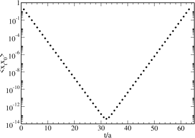
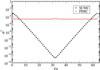
In the left plot of Figure 1 we show the two-point correlation function computed on a lattice with $N=64$ points, with statistical errors being smaller than symbols. The error (SCMC) is shown on the right plot of the same Figure. The signal-to-noise ratio is depleted, as expected, (only) inversely proportional to the time distance of the sources. For comparison in the same plot it is also shown the statistical error obtained with a standard Monte Carlo procedure (PIMC) which needed roughly the same CPU time. It is clear that with our strategy the statistical error is exponentially reduced, and at large time distances it is lowered by many orders of magnitude.

Figure 1: Left: two-point correlation function versus the time distance $t/a$ of the sources. Right: errors on the correlation function as obtained with the multi-level algorithm (SCMC) and with the standard path integral Monte Carlo (PIMC).

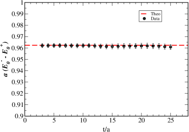
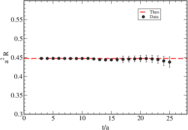
The effective energy-split $a\tilde{\omega}(t)$ extracted from the correlator is shown in the left plot of Figure 2, and it is in perfect agreement with the theoretical expectation [6]. On the right plot of the same figure it is shown the effective estimate $R(t)$ of the square of the matrix element $\langle{\cal{E}}_{0}^{-}|\hat{x}|{\cal{E}}_{0}^{+}\rangle$ computed as

$$R(t)=\frac{\langle x_{l}x_{k}\rangle\;e^{\tilde{\omega}\frac{T}{2}}}{2\cosh{\left[\tilde{\omega}\left(\frac{T}{2}-a|l-k|\right)\right]}}\;,$$ (16)

which also agrees very well with the analytical result.

Figure 2: Left: effective energy difference extracted from the two-point correlator at any time separation $t/a$. Right: the ratio $R$ as defined in the text.

The approach described here is of inspiration for systems with a larger number of degrees of freedom. In that case, however, one cannot make sense of the “sign” and “module” fields. New concepts have to be introduced as we illustrate in the following for the $SU(3)$ Yang-Mills theory [4].

2 Extension to Yang-Mills theories on the lattice

We again divide the parity even sector of the theory from the parity odd, naming the energy levels $E_{i}^{+}$ and $E_{j}^{-}$ respectively. The statistical variance of the estimate of a two-point correlation function $\langle O(x_{0})O(0)\rangle$ of a parity-odd interpolating operator $O$, computed by the standard Monte Carlo procedure, is defined as

$$\sigma^{2}=\langle O^{2}(x_{0})O^{2}(0)\rangle-\langle O(x_{0})O(0)\rangle^{2}\;.$$ (17)

At asymptotically-large time separations the signal-to-noise ratio takes the form

$$\frac{\langle O(x_{0})O(0)\rangle}{\sigma}=\frac{|\langle E_{1}^{-}|\hat{O}|0\rangle|^{2}}{|\langle 0|\hat{O}^{2}|0\rangle|}\,e^{-E_{1}^{-}x_{0}}+\cdots$$ (18)

i. e. the signal is again depleted exponentially in time.

For the one-dimensional harmonic oscillator the quantity $\tanh\{a\,\Lambda^{-}_{m+1,m}\}$ represented the ratio $Z^{-}/Z^{+}$ for a system of one time-slice with fixed boundary configurations. Due to the regularity of the spectrum this ratio is of O$(1)$. The same cannot be expected for systems with many degrees of freedom, as the four-dimensional Yang-Mills theory, the ratio will rather be of O$(e^{-(L/a)^{3}})$, with $L$ the spatial extent of the lattice. However, if one considers systems $d$ time-slices large, with $d\sim 1/T_{\rm c}$ and $T_{\rm c}$ the critical temperature, the same ratio is now expected to be of O($e^{-E_{1}^{-}d}$) for each boundary configuration. These are the quantities we want to directly access and use to rewrite our observables. To this end we first need to briefly recall the formalism of the transfer matrix, we refer to [4] for a more thorough discussion.

2.1 Transfer matrix

We adopt Wilson’s regularization of gauge theories [7]. The corresponding transfer matrix has been explicitly constructed in [8, 9, 10, 11]. The functional integral with periodic boundary conditions in time can be written as

$$Z=\int\prod_{x_{0}=0}^{T-1}\,{\rm\bf D}_{3}[V_{x_{0}}]\,{\rm T}\Big{[}V_{x_{0}+1},V_{x_{0}}\Big{]}$$ (19)

where the transfer matrix elements among states $|V_{x_{0}}\rangle$ in the coordinate basis are defined as

$${\rm T}\Big{[}V_{x_{0}+1},V_{x_{0}}\Big{]}=\int{\rm\bf D}[\Omega]\;e^{-L[V^{\Omega}_{x_{0}+1},V_{x_{0}}]}\;,$$ (20)

with

$$L\Big{[}V_{x_{0}+1},V_{x_{0}}\Big{]}=K\Big{[}V_{x_{0}+1},V_{x_{0}}\Big{]}+\frac{1}{2}W\Big{[}V_{x_{0}+1}\Big{]}+\frac{1}{2}W\Big{[}V_{x_{0}}\Big{]}\;,$$ (21)

and $|V_{x_{0}}^{\Omega}\rangle$ is the result of a gauge transformation $\Omega$ on the state $|V_{x_{0}}\rangle$. The kinetic and the potential contributions to the Lagrangian are given by

$$K\Big{[}V_{x_{0}+1},V_{x_{0}}\Big{]}=\beta\sum_{{\bf x},k}\left[1-\frac{1}{3}{\rm Re}\,\hbox{\rm Tr}\left\{V_{k}(x_{0}+1,{\bf x})V^{\dagger}_{k}(x_{0},{\bf x})\right\}\right]\;,$$ (22)

and

$$W\Big{[}V_{x_{0}}\Big{]}=\frac{\beta}{2}\sum_{{\bf x}}\sum_{k,l}\left[1-\frac{1}{3}{\rm Re}\,\hbox{\rm Tr}\Big{\{}V_{kl}(x_{0},{\bf x})\Big{\}}\right]\;,$$ (23)

respectively, where $V_{kl}$ is the spatial plaquette computed with the links $V_{k}({\bf x})$. By exploiting the invariance of the Haar integration measure under left and right multiplication it is easy to show that the transfer matrix is gauge invariant. For a thick time-slice, i.e. the ensemble of points in the sub-lattice with time coordinates in a given interval $[x_{0},y_{0}]$ and bounded by the equal-time hyper-planes at times $x_{0}$ and $y_{0}$, the transfer matrix elements can be introduced by the formula

$${\rm T}\Big{[}V_{y_{0}},V_{x_{0}}\Big{]}=\int\prod_{w_{0}=x_{0}+1}^{y_{0}-1}\,{\rm\bf D}_{3}[V_{w_{0}}]\,\prod_{z_{0}=x_{0}}^{y_{0}-1}{\rm T}\Big{[}V_{z_{0}+1},V_{z_{0}}\Big{]}\;.$$ (24)

The parity transformation acts on the states in the coordinate basis as

$$\mbox{ $\hat{\wp}$}\,|{\rm V}\rangle=|{\rm V}^{\wp}\rangle\;,\qquad|{\rm V}\rangle=\hat{{\rm P}}_{\rm G}|V\rangle\;,\qquad V^{\wp}_{k}({\bf x})=V^{\dagger}_{k}(-{\bf x}-\hat{k})\;,$$ (25)

where $\hat{{\rm P}}_{\rm G}$ is the projector on gauge invariant states. Again, we can then define a complete set of parity eigenstates

$$|{\rm V},\pm\rangle=\frac{1}{\sqrt{2}}\Big{[}|{\rm V}\rangle\pm|{\rm V}^{\wp}\rangle\Big{]}\;,\qquad\mbox{ $\hat{\wp}$}\,|{\rm V},\pm\rangle=\pm|{\rm V},\pm\rangle\;,$$ (26)

and their transfer matrix elements are given by

$$\langle s^{\prime},{\rm V}_{x_{0}+1}|\hat{\rm T}|{\rm V}_{x_{0}},s\rangle = 2\,\delta_{s^{\prime}s}\;{\rm T}^{s}\Big{[}V_{x_{0}+1},V_{x_{0}}\Big{]}\;,$$ (27)

$${\rm T}^{s}\Big{[}V_{x_{0}+1},V_{x_{0}}\Big{]} = \frac{1}{2}\left\{{\rm T}\Big{[}V_{x_{0}+1},V_{x_{0}}\Big{]}+s\,{\rm T}\Big{[}V_{x_{0}+1},V^{\wp}_{x_{0}}\Big{]}\right\}\;.$$ (28)

For a thick time-slice the matrix elements between parity states can be introduced by exploiting the same composition rule as in Eq. (24) with $\rm T$ replaced by ${\rm T}^{s}$. In addition, the relations

$$\int{\rm\bf D}_{3}[V_{z_{0}}]\,{\rm T}^{s}\Big{[}V_{y_{0}},V_{z_{0}}\Big{]}\;{\rm T}^{-s}\Big{[}V_{z_{0}},V_{x_{0}}\Big{]} = 0\;,$$ (29)

$$\int{\rm\bf D}_{3}[V_{z_{0}}]\,{\rm T}^{s}\Big{[}V_{y_{0}},V_{z_{0}}\Big{]}\;{\rm T}\Big{[}V_{z_{0}},V_{x_{0}}\Big{]} = {\rm T}^{s}\Big{[}V_{y_{0}},V_{x_{0}}\Big{]}$$ (30)

hold. In particular they imply that

$$\frac{{\rm T}^{s}[V_{y_{0}},V_{x_{0}}]}{{\rm T}\;[V_{y_{0}},V_{x_{0}}]}=\frac{1}{Z_{\mathrm{sub}}}\int{\rm D}_{4}[U]_{\mathrm{sub}}\;e^{-S[U]}\,\frac{{\rm T}^{s}[U_{y_{0}},U_{y_{0}-1}]}{{\rm T}\,[U_{y_{0}},U_{y_{0}-1}]}\;,$$ (31)

an useful expression for the practical implementation of the multi-level algorithm described in the following. The subscript “sub” indicates that the integral is performed over the dynamical field variables in the thick time-slice $[x_{0},y_{0}]$ with the spatial components $U_{k}(x)$ of the boundary fields fixed to $V_{k}(x_{0},\vec{\bf x})$ and $V_{k}(y_{0},\vec{\bf x})$ respectively. Finally, by replacing ${\rm T}[V_{x_{0}+1},V_{x_{0}}]$ in Eq. (19) by $\sum_{s}{\rm T}^{s}[V_{x_{0}+1},V_{x_{0}}]$ and repeatedly applying Eq. (29), it is possible to rewrite the path integral as a sum of functional integrals

$$Z=\sum_{s=\pm}Z^{s}\;,\qquad Z^{s}=\int\prod_{x_{0}=0}^{T-1}\,{\rm\bf D}_{3}[V_{x_{0}}]\,{\rm T}^{s}\Big{[}V_{x_{0}+1},V_{x_{0}}\Big{]}\;,$$ (32)

each giving the contribution from gauge-invariant parity-even and -odd states respectively.

The insertion of ${\rm T}^{s}[V_{y_{0}},V_{x_{0}}]$ in the path integral plays the rôle of a projector, as on each configuration it allows the propagation in the time direction of states with parity $s$ only. Indeed the parity transformation of one of the boundary fields in ${\rm T}[V_{y_{0}},V_{x_{0}}]$ flips the sign of all contributions that it receives from the parity-odd states while leaving invariant the rest. The very same applies to the path integral in Eq. (19) if the periodic boundary conditions are replaced by $\wp$-periodic boundary conditions, i.e. $V_{T}=V^{\wp}_{0}$. All contributions from the parity odd states are then multiplied by a minus sign.

2.2 The hierarchical integration scheme

To determine the parity projector between two boundary fields of a thick time-slice, the basic building block to be computed is the ratio of transfer matrix elements

$${\rm R}[V_{x_{0}+d},V_{x_{0}}]=\frac{{\rm T}[V_{x_{0}+d},V^{\wp}_{x_{0}}]}{{\rm T}[V_{x_{0}+d},V_{x_{0}}]}\;.$$ (33)

As mentioned above, for $d$ of $O(1/T_{\rm c})$, the ratio $R$ is expected to be of $O(1)$. However the integrands in the numerator and in the denominator on the r.h.s of Eq. (33) are, in general, very different and the main contributions to their integrals come from different regions of the phase space. The most straightforward way for computing $R$ is to define a set of $n$ systems with partition functions ${\cal Z}_{1}\,\dots\,{\cal Z}_{n}$ designed in such a way that the relevant phase spaces of successive integrals overlap and that ${\cal Z}_{1}={\rm T}[V_{x_{0}+d},V^{\wp}_{x_{0}}]$ and ${\cal Z}_{n}={\rm T}[V_{x_{0}+d},V_{x_{0}}]$. The ratio $R$ can then be calculated as

$${\rm R}=\frac{{\cal Z}_{1}}{{\cal Z}_{2}}\times\frac{{\cal Z}_{2}}{{\cal Z}_{3}}\times\dots\times\frac{{\cal Z}_{n-2}}{{\cal Z}_{n-1}}\times\frac{{\cal Z}_{n-1}}{{\cal Z}_{n}}\;,$$ (34)

with each ratio on the r.h.s. being computable in a single Monte Carlo simulation by averaging the proper reweighting factor.

For the case at hand ${{\cal Z}_{1}}$ and ${{\cal Z}_{n}}$ are the partition functions of two systems differing only for the boundary conditions in time. In both cases Dirichlet boundary conditions are imposed but the boundary configurations at time $x_{0}+d$ differ by a parity transformation. Instead of relating the boundary configurations in such a way, we change the action of one of the two systems on the last time-slice, by introducing a new temporal link connecting the point ${\mathbb{x}},x_{0}+d-1$ on the last dynamical time-slice to its parity transformed $-{\mathbb{x}},x_{0}+d$ on the boundary. We call the associated plaquette “parity twisted” space-time plaquette and $K^{\wp}$ (parity twisted kinetic term) the sum of such plaquettes (see Figure 3).

Figure 3: Two dimensional representation of the plaquettes in the kinetic terms $K$ ($r=1/2$) and $K^{\wp}$ ($r=-1/2$) on the time-slice $y_{0}-1$. The telescopic algorithm described in the text bridges between the two systems in $L^{3}$ steps.

To interpolate between the two systems we slowly switch off the coupling $\beta$ in $K$ by decreasing it in steps of size $\epsilon=1/L^{3}$ while increasing the coupling in $K^{\wp}$ by the same amount, we distinguish the interpolating actions by a parameter $-1/2\leq r\leq 1/2$. In this way we move in $L^{3}$ steps from one system to the other. This means we need to perform a chain of $L^{3}$ Monte Carlo simulations within a Monte Carlo simulation and we therefore have an algorithm, which scales with the second power of the volume $L^{3}$. This is the case also for other known methods for computing ratios of partition functions [12, 13, 14].

Once the projectors have been computed, the ratio of partition functions $Z^{s}/Z$ can be calculated by implementing the hierarchical two-level integration formula

$$\frac{Z^{s}}{Z}=\frac{1}{Z}\int{\rm D}_{4}[U]\,e^{-S[U]}\,{{\rm P}}^{s}_{m,d}\Big{[}T,0\Big{]}$$ (35)

where ${\rm P}^{s}_{m,d}\Big{[}y_{0},x_{0}\Big{]}$ is defined as

$${{\rm P}}^{s}_{m,d}\Big{[}y_{0},x_{0}\Big{]}={\prod_{i=0}^{m-1}}\frac{{\rm T^{s}}[U_{x_{0}+(i+1)\cdot d},U_{x_{0}+i\cdot d}]}{{\rm T}[U_{x_{0}+(i+1)\cdot d},U_{x_{0}+i\cdot d}]}$$ (36)

with $m\geq 1$ and $y_{0}=x_{0}+m\cdot d$. The procedure can, of course, be generalized to a multi-level algorithm. For a three-level one, for instance, each ratio on the r.h.s of Eq. (36) can be computed by a two-level scheme. For each configuration of the boundary fields, the magnitude of the product in our observable ${{\rm P}}^{s}_{m,d}[T,0]$ is proportional to $e^{-E^{-}_{1}\,T}$, and the statistical fluctuations are reduced to this level. This has to be compared to the standard case in which each configuration gives a contribution to the signal which decreases exponentially in time, whereas it contributes $O(1)$ to the noise (variance) at any time distance. To achieve an analogous exponential gain in the computation of the correlation functions, the projectors ${\rm T^{s}}$ have to be inserted in the proper way among the interpolating operators. As a technical aside we remark that the computation of $\rm R$ requires a thermalization procedure for each value of $r$. We do not expect the latter to be particularly problematic since, as mentioned above, expectation values for consecutive values of $r$ refer to path integrals with the relevant phase spaces which overlap. The ratio $\rm R$ is computed by simulating systems corresponding to consecutive values of $r$ one after the other, and by starting from the one used to extract the boundary fields ($r=1/2$).

2.3 Results

In the four-dimensional SU(3) Yang-Mills theory we have simulated lattices with an inverse gauge coupling of $\beta=6/g^{2}_{0}=5.7$ which corresponds to a value of the reference scale $r_{0}$ of about $2.93a$ [15, 16]. The number of lattice points in each spatial direction has been set to $L=6,8$ and $10$ corresponding to a linear size of $1.0$, $1.4$ and $1.7$ fm respectively. For each spatial volume we have considered several time extents $T$, the full list is reported in Table 1 together with the number of configurations generated, the details of the multi-level simulation algorithm used for each run and the results for $Z^{-}/Z$ and for the effective mass $M^{-}$ of the first parity-odd glueball state extracted from that ratio:

$$M^{-}=-\frac{1}{T}\ln\left(\frac{Z^{-}}{Z}(T)\right)\;.$$ (37)

Lattice	$L$	$T$	$N_{\mathrm{conf}}$	$N_{\mathrm{lev}}$	$d$	${{Z^{-}}\over{Z}}$	$aM^{-}$
${\rm A}_{1}$	6	4	50	2	4	0.409(8)	0.223(5)
${\rm A}_{2}$		5	50	2	5	0.177(13)	0.346(14)
${\rm A}_{3}$		6	50	2	6	0.069(7)	0.446(17)
${\rm A}_{4}$		8	175	2	4	1.47(28)$\cdot 10^{-2}$	0.528(24)
${\rm A}_{5}$		10	50	2	5	2.2(5)$\cdot 10^{-3}$	0.611(20)
${\rm A}_{6}$		12	90	2	6	6.6(17)$\cdot 10^{-4}$	0.610(21)
${\rm A}_{7}$		16	48	2	8	2.8(8)$\cdot 10^{-5}$	0.655(18)
${\rm A}_{8}$		20	48	3	{5,10}	1.5(5)$\cdot 10^{-6}$	0.670(15)
${\rm B}_{1}$	8	4	20	2	4	0.426(8)	0.213(5)
${\rm B}_{2}$		5	25	2	5	0.061(6)	0.558(21)
${\rm B}_{3}$		6	75	2	3	1.65(26)$\cdot 10^{-2}$	0.685(27)
${\rm B}_{4}$		8	48	2	4	1.37(26)$\cdot 10^{-3}$	0.824(24)
${\rm B}_{5}$		12	48	3	{3,6}	3.6(18)$\cdot 10^{-6}$	1.045(41)
${\rm B}_{6}$		16	36	3	{4,8}	5.2(19)$\cdot 10^{-8}$	1.048(23)
${\rm C}_{1}$	10	4	20	2	4	0.455(12)	0.197(6)
${\rm C}_{2}$		5	24	2	5	0.060(3)	0.561(11)
${\rm C}_{3}$		6	50	2	3	1.6(4)$\cdot 10^{-2}$	0.687(39)
${\rm C}_{4}$		8	48	2	4	5.2(16)$\cdot 10^{-4}$	0.944(39)
${\rm C}_{5}$		12	24	3	{3,6}	3.3(17)$\cdot 10^{-6}$	1.052(43)

Table 1: Simulation parameters and results. $N_{\mathrm{conf}}$ is the number of configurations of the uppermost level, $N_{\mathrm{lev}}$ is the number of levels and $d$ is the thickness of the thick time-slice used for the various levels. The effective mass $M^{-}$ is given by $-T^{-1}\ln(Z^{-}/Z)$.

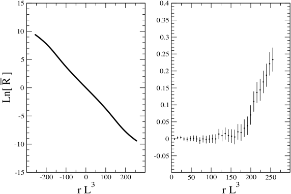
The natural logarithm of $\frac{{\cal Z}_{i-1}}{{\cal Z}_{i}}$ for the interpolating systems in Eq. (34) is shown as a function of $r$ in the left panel of Fig. 4 for a typical configuration of the run ${\rm B}_{3}$. As expected, its value is of $O(1)$ for each value of $r$. Its almost perfect asymmetry under $r\rightarrow-r$, however, makes the product of all the $L^{3}$ results a quantity of $O(1)$. This impressive cancellation, which is at work for $T>3$ on all volumes considered, can be better appreciated in the right panel of the same Figure, where the sum of the function in the interval $[-r,r]$ is plotted for a subset of values of $r$. It is the deviation from the exact asymmetry which flips in sign under a parity transformation of one of the boundary fields, and forms the signal we are interested in.

Figure 4: Left: the natural logarithm of $\frac{{\cal Z}_{i-1}}{{\cal Z}_{i}}$ is shown as a function of $r$ (statistical errors are smaller than symbols) for a typical configuration of the run ${\rm B}_{3}$. Right: the sum of the points in the interval $[-r,r]$ is plotted as a function of $r$ (one each eighth point for visual convenience).

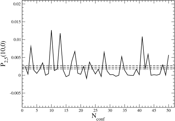
The Monte Carlo history of ${{\rm P}}^{-}_{2,T/2}[T,0]$ is shown in Figure 5 for the lattice ${\rm A}_{5}$. The central dashed line corresponds to the average value, while the other two delimit the one standard deviation region. As expected the Monte Carlo history is very regular and each configuration gives an estimate of the observable which is of the right size. Fluctuations are five times the average value at most. We have observed similar Monte Carlo histories also for the other runs.

Figure 5: Monte Carlo history of the quantity ${{\rm P}}^{-}_{2,5}[10,0]$ for the run ${\rm A}_{5}$.

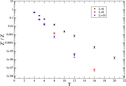
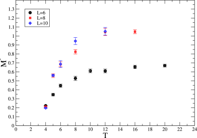
Finally we show the results for $Z^{-}/Z$ and $aM^{-}$ in Figs. 6 and 7 respectively. We have been able to follow the exponential decay in the ratio $Z^{-}/Z$ over almost 7 orders of magnitude. The data at large values of $T/a$ can be used to estimate the multiplicity of the first parity odd state, a quantity which is not accessible within the other approaches. To this end the precision however has to be increased, as for now we assume the multiplicity to be one, which justifies the definition of the effective mass $M^{-}$ in Eq. 37. Figure 7 shows that the algorithm works as expected as the error on the effective mass could be kept constant to the level of a few percent up to a separation of about $3.5$ fm. It also shows that finite size effects are rather large for lattices of linear size around $1$ fm ($L/a=6$) but they become negligible within the present accuracy once a size of $1.4$ fm ($L/a=8$) is reached. We therefore quote $r_{0}m_{G^{-}}=3.07(7)$ from $L/a=8$, $T/a=16$ as a preliminary result for the mass of the lightest $J^{PC}=0^{-+}$ glueball at a lattice resolution of $0.17$ fm with Wilson’s gauge action. Given the quite large value of the lattice spacing, cutoff effects may affect this number significantly.

Figure 6: The quantity $Z^{-}/Z$ vs $T/a$.

Figure 7: The quantity $aM^{-}$ vs $T/a$.

3 Conclusions and outlook

For most of the two-point functions computed on the lattice the noise to signal ratio grows exponentially with the time separation of the source and the sink. This disease can be cured by imposing the propagation of states with the desired quantum numbers only on each (gauge) configuration. The algorithm proposed here solves the problem by making use of the symmetry properties of the underlying quantum theory. We have numerically tested the approach in the four-dimensional SU(3) Yang-Mills theory, by computing the mass of the lightest parity-odd glueball. For a given precision on the latter the algorithm scales as a power of $T$, the total time extent of the lattice, and we have therefore been able to follow an exponential decay over 7 orders of magnitude and up to separations of $3.5$ fm. That allows to isolate the contribution of a single state with unprecedented confidence. We have also studied finite size effect and collected strong indications that, for the effective mass considered here and within our statistical errors, those are negligible for $L>1.4$ fm. The multiplicity of the state can also be computed using the approach described, and in the near future we plan to increase the accuracy on its determination, which can be obtained only with limited precision by using the data produced so far. The reduction of systematic uncertainties related to lattice artifacts remains an expensive task as the algorithm scales roughly as $(L/a)^{6}$.

The inclusion of other symmetries is straightforward. We have already implemented charge-conjugation and tested it in small volumes, observing basically the same efficiency of the integration scheme as for the parity discussed here. Different symmetry transformations can be actually considered simultaneously and we plan to include cubic rotations and translations. The mass of the lightest state in any sector specified by the quantum numbers $J^{PC}$ could then be computed without suffering from the exponential problem [17].

A way to generalize the ideas reported here to systems including fermion degrees of freedom is, at present, not known. Among other advantages, such an extension would allow to compute the ratio between the partition functions at different baryon quantum numbers avoiding the sign problem, which affects the simulations at finite density.

References

- [1] G. Parisi, Phys. Rept. 103 (1984) 203.
- [2] G.P. Lepage, TASI 89 Summer School, Boulder, CO, Jun 4-30, 1989.
- [3] M. Della Morte and L. Giusti, Comput. Phys. Commun. 180 (2009) 813.
- [4] M. Della Morte and L. Giusti, Comput. Phys. Commun. 180 (2009) 819, arXiv:0806.2601 [hep-lat].
- [5] M. Lüscher and P. Weisz, JHEP 09 (2001) 010, hep-lat/0108014.
- [6] M. Creutz and B. Freedman, Ann. Phys. 132 (1981) 427.
- [7] K. G. Wilson, Phys. Rev. D 10, 2445 (1974).
- [8] K.G. Wilson, in ”New developments in quantum field theory and statistical mechanics”, Cargèse 1976, Eds. M. Lévy and P. Mitter, Plenum (NY 1977).
- [9] M. Lüscher, Commun. Math. Phys. 54 (1977) 283.
- [10] M. Creutz, Phys. Rev. D15 (1977) 1128.
- [11] K. Osterwalder and E. Seiler, Ann. Phys. 110 (1978) 440.
- [12] A.M. Ferrenberg and R.H. Swendsen, Phys. Rev. Lett. 63 (1989) 1195.
- [13] C. Hoelbling, C. Rebbi and V.A. Rubakov, Phys. Rev. D63 (2001) 034506, hep-lat/0003010.
- [14] P. de Forcrand, M. D’Elia and M. Pepe, Phys. Rev. Lett. 86 (2001) 1438, hep-lat/0007034.
- [15] ALPHA Coll., M. Guagnelli, R. Sommer and H. Wittig, Nucl. Phys. B535 (1998) 389, hep-lat/9806005.
- [16] S. Necco and R. Sommer, Nucl. Phys. B622 (2002) 328, hep-lat/0108008.
- [17] M. Della Morte and L. Giusti, in preparation.