Activity Dependent Branching Ratios in Stocks, Solar X-ray Flux, and the Bak-Tang-Wiesenfeld Sandpile Model

Abstract

We define an activity dependent branching ratio that allows comparison of different time series $X_{t}$. The branching ratio $b_{x}$ is defined as $b_{x}=E[\xi_{x}/x]$. The random variable $\xi_{x}$ is the value of the next signal given that the previous one is equal to $x$, so $\xi_{x}=\{X_{t+1}|X_{t}=x\}$. If $b_{x}>1$, the process is on average supercritical when the signal is equal to $x$, while if $b_{x}<1$, it is subcritical. For stock prices we find $b_{x}=1$ within statistical uncertainty, for all $x$, consistent with an “efficient market hypothesis”. For stock volumes, solar X-ray flux intensities, and the Bak-Tang-Wiesenfeld (BTW) sandpile model, $b_{x}$ is supercritical for small values of activity and subcritical for the largest ones, indicating a tendency to return to a typical value. For stock volumes this tendency has an approximate power law behavior. For solar X-ray flux and the BTW model, there is a broad regime of activity where $b_{x}\simeq 1$, which we interpret as an indicator of critical behavior. This is true despite different underlying probability distributions for $X_{t}$, and for $\xi_{x}$. For the BTW model the distribution of $\xi_{x}$ is Gaussian, for $x$ sufficiently larger than one, and its variance grows linearly with $x$. Hence, the activity in the BTW model obeys a central limit theorem when sampling over past histories. The broad region of activity where $b_{x}$ is close to one disappears once bulk dissipation is introduced in the BTW model – supporting our hypothesis that it is an indicator of criticality.

I Introduction

Detailed forecasting in complex systems is often difficult if not impossible. Nonlinear processes as well as long range spatial and/or temporal correlations can render a direct, reductionist approach futile. Furthermore, in many cases of interest, controlled laboratory experiments are unfeasible. For instance, stock market data or solar X-ray flux can only be obtained under specific conditions set by the system itself, and observing the time series under various controlled conditions is not possible.

Testing the efficient market hypothesis (EMH) presents a clear example of this difficulty. Roughly speaking, the EMH states that asset prices are inherently unpredictable Samuelson (1965); Mandelbrot (1966); F. (1989), or that the market is hard to beat McCauley et al. (2008). There are many flavors of the EMH. The weak EMH states that the market is efficient if agents only have information about the time series of market prices. The strong EMH, on the other hand, states that the market is efficient when agents have access to all relevant information that could affect prices; this includes e.g. insider trading.

Mathematically the weak EMH can be formulated in terms of a martingale property for the time series of prices Fama (1970). In its simplest form, a stochastic variable, $X_{t}$, is said to be a martingale if the expectation of its next value given its entire past is equal to its current value, or $E[X_{t+1}|X_{t}...X_{0}]=X_{t}$ for all $t$. Empirically, it is not possible to obtain this expectation value directly from real world time series. In fact, the existence of EMH in any of its forms is highly disputed Farmer and Lo (1999); Lo (2004).

For a Markov process, the value that $X_{t+1}$ takes only depends on the previous value $X_{t}$. Indeed a necessary but not sufficient requirement for any stochastic process to be a Martingale is that $E[X_{t+1}|X_{t}]=X_{t}$. One example is the critical Galton-Watson (GW) branching process Lyons and Peres (In preparation). Starting with a single node, $X_{0}=1$, each node independently produces a number of offspring that is Poisson distributed with mean $b$. Here $b$ is called the branching ratio. If $b=1$ the process is critical and is also a Martingale, since $E[X_{t+1}|X_{t}...X_{0}]=E[X_{t+1}|X_{t}]=bX_{t}$.

If the underlying probability distribution used to evaluate the expectation value $E[\cdots]$ is not known, or if the nodes interact with each other in generating offspring, one can still empirically measure an activity dependent branching ratio as $b_{x}=E[\xi_{x}/x]$. Here the random variable $\xi_{x}$ is the value of the next signal given that the previous one is equal to $x$, or $\xi_{x}=\{X_{t+1}|X_{t}=x\}$. We interpret $\xi_{x}$ as the set of outcomes of an interacting branching process with a current population $x$. Empirically the expectation value $E[\xi_{x}/x]$ is an average over all times $t$ when $X_{t}=x$. If $b_{x}=1$ the process is on average critical when the activity is equal to $x$. If $b_{x}>1$, it is supercritical and if $b_{x}<1$ it is subcritical. Note that we are not making any assumptions that the processes we measure are, in fact, Markovian. The measured branching ratio $b_{x}$ is an average over all observed histories leading to a population of size $x$.

We use the activity dependent branching ratio $b_{x}$ to compare and contrast time series from stock markets, a physical system (solar X-ray flux) and a model (the Bak-Tang-Wiesenfeld (BTW) sandpile). Previously, time series of activity in the BTW sandpile have been compared in detail with that of solar flux – finding a number of similarities Paczuski et al. (2005). Our analysis finds similarities as well as significant differences in these two systems.

We find that $b_{x}$ is statistically indistinguishable from unity for time series of stock prices as well as for the Dow Jones industrial average, consistent with the weak EMH. On the other hand, stock volumes, X-ray flux and activity in the BTW model all show roughly similar behavior: $b_{x}$ decreases from a supercritical value at low levels of activity to a subcritical one at large values. This indicates a general tendency for the activity to return to a characteristic value, which is not present for stock prices. For stock volumes, the branching ratio has a relatively strong dependence on activity, $b_{V}\sim\left(V/\langle V\rangle\right)^{-\alpha}$ with $\alpha\simeq 0.69$. Solar X-ray flux and activity in the BTW model both show a broad range of activity where the branching ratio is close to one. This broad range increases with the system size for the BTW model and disappears once bulk dissipation is introduced, suggesting that it is an indicator of criticality.

We also compare and contrast the probability distributions $P(\xi_{x}/x)$, at particular values of activity $x$ in these systems. For the BTW model, this distribution is well described by a Gaussian for x sufficiently larger than 1. On the other hand, for both stock volumes and flux intensities, $P(\xi_{x}/x)$ is broader than Gaussian. The marginal distribution of flux intensities $P(I)$ is well described by a power law, while for the BTW model the distribution of activity $P(n)$ is approximately exponential with a correlation length that grows with system size.

In Section II, we present results for the branching ratios determined from analyses of time series for stock prices and for stock volumes considering four different stocks as well as the daily Dow Jones average. Section III presents results for solar X-ray flux data. Section IV contrasts and compares results for the canonical BTW model with variants (a) including bulk dissipation – making the model subcritical, and (b) having periodic boundary conditions, which leads to non-ergodic behavior. We also discuss how our activity dependent branching ratio differs from the average branching ratio for avalanches in self-organized critical (SOC) systems previously discussed in the literature (See e.g. Refs. de Carvalho and Prado (2000); Christensen et al. (2001)). Section V contains a discussion and summary of the main results.

II Stock Market

Does knowledge of the current price or volume of trade for a particular stock or market index allow one to make predictions about the next value? For prices the answer is no, while for volume of trade the answer is yes, as discussed next.

We analyze one minute resolution data for four different stocks from His for intervals of $28$ days. We also examine one day resolution data for the Dow Jones over $80$ years from Yah . Both price $\xi_{P}=\{P(t+1)|P(t)=P\}$, and volume $\xi_{V}=\{V(t+1)|V(t)=V\}$ are studied.

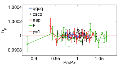
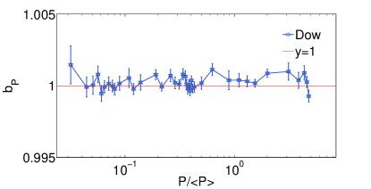
Fig. 1 shows the activity dependent branching ratio $b_{p}=E[\xi_{p}/P]$ vs. $P/\langle P\rangle$ for four different stocks. The same quantity for the Dow Jones is shown in Fig. 2. The symbol $\langle\cdots\rangle$ indicates an average over the observation time. For all price time series studied $b_{p}=1$ within statistical uncertainty. These data are binned such that there are at least 500 points in each bin, and error bars indicate one standard deviation.

Figure 1: (color on-line) The branching ratio $b_{p}$ vs. price for different stocks. The x-axis has been scaled by the mean price. All data shown have a resolution of one minute, where the price used is that at the start of the minute. Error bars in this and subsequent figures indicate one standard deviation. The data for qqqq was taken over the period 09:30 23/05/08 - 13:37 20/06/08, the data for csco is from 09:30 23/05/08 - 13:37 20/06/08, the data for aapl is from 9:30 27/05/08 - 14:08 23/06/08, the data for F is from 09:30 27/05/08 - 14:03 23/06/08. These results are consistent with the weak EMH.

Figure 2: (color on-line) Same as Fig. 1 for the Dow Jones industrial average. The data is from 01/10/1928 - 23/05/2008, and has a resolution of 1 day using the opening price. The behavior is also consistent with the weak EMH.

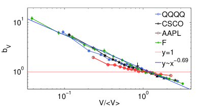
The activity dependent branching ratio for volume, $b_{V}$, has a strong dependence on volume as shown in Fig. 3. For small values the stocks behave like a supercritical branching process, while for large values they are subcritical. Hence the volume has a tendency to return to roughly its mean value. In fact, $b_{V}$ has an approximate power law dependence on $V$, with $b_{V}\sim\left(V/\langle V\rangle\right)^{-\alpha}$. The exponent $\alpha\simeq 0.69$ for three of the stocks shown in Fig. 3 but appears to be smaller (or nonexistent) for the Apple stock (aapl), which also has a more limited variation in volume, precluding any firm conclusion about scaling. We have also analyzed this quantity for different time windows (data not shown) and the results for the individual stocks do not vary in any substantial way. The data for the Dow Jones volumes (not shown) are too noisy to draw definite conclusions.

Figure 3: (color on-line) Activity dependent branching ratios for stock volumes during the same time period as in Fig. 1. A line with slope $m=-0.69$ is included as a guide for the eye. The behavior of the Apple stock (aapl) appears to deviate from the other three.

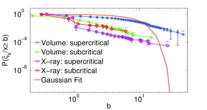
For a given level of activity, the probability distribution $P(\xi_{V}/V)$, also differs significantly from that for prices $P(\xi_{P}/P)$. For prices we find results similar to that found in Ref. Mantegna and Stanley (1995), who analyzed price changes for different time increments over all prices. In our case the data (not shown) are much more noisy since we fix both the initial value of price, as well as the time interval (one minute). For stock volumes and solar intensities, the cumulative distributions $P(\xi_{V}/V\geq b)$ at a given $V$ and $P(\xi_{I}/I\geq b)$ at a given $I$, are both broader than Gaussian as shown in Fig. 4.

Figure 4: (color on-line) Comparison of cumulative distribution function (CDF) $P(\xi_{x}/x\geq b)$ for stock volumes and solar intensities at a given value of activity $x$. For stock volumes, Ford (F) was used, and the CDFs calculated at $x=V/\langle V\rangle=0.2\pm 0.05$ (supercritical region) and $x=V/\langle V\rangle=2\pm 1$ (subcritical). For solar intensities the entire time series, “All”, was used, and the CDFs calculated at $x=I/\langle I\rangle=0.1\pm 0.005$ (supercritical) and $x=I/\langle I\rangle=100\pm 10$ (subcritical). The Ford CDF at $x=0.2\pm 0.05$ is compared with a Gaussian having the same mean and variance. The distributions are broader than Gaussian in all cases.

III Solar X-ray Flux

Figure 5: (color on-line) Activity dependent branching ratios for solar flux intensity at solar minimum, solar maximum, and for the entire data set, “All”, as defined in the text. This shows a weak tendency to return to a typical value although $b_{I}\approx 1$ for a broad range of intensities, $I$. This behavior is comparable to that shown for the SOC BTW model in Fig. 7.

Figure 6: (color on-line) The probability distribution function of solar x-ray intensities, $P(I)$. The straight line indicates a power law fit with exponent $2.3$ for the “All” time series. This is different from the approximately exponential behavior seen in the SOC BTW model as shown in Fig. 8.

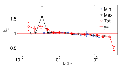
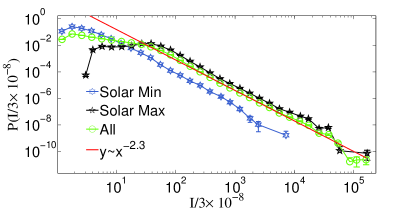
Solar flares are bursts of radiation that occur in the solar corona. These bursts can reach sufficiently high energies to pose a risk to astronauts, spacecraft, or airplanes following polar routes. In addition they exhibit a number of empirical features associated with SOC Paczuski et al. (2005); Baiesi et al. (2006); Uritsky et al. (2007); Lu and Hamilton (1991); Paczuski and Hughes (2004); Charbonneau et al. (2001). For instance, the distribution of event durations and quiet times is a power-law for both solar flux and the BTW sandpile Paczuski et al. (2005), once physically relevant detection thresholds are taken into account to compare these time series on an equal basis. Our analysis shows that the dependence of the branching ratio on activity are similar in the two cases although the underlying probability distributions for activity $(X_{t})$ and for subsequent conditioned activities $\xi_{x}$ are different.

We examine time series in the $1-8$Å range obtained from the Geostationary Operational Environmental Satellites (GOES) Satellites at the “Space Physics Interactive Data Resource” SPI . A time series of five minute intervals from 01/01/1986 to 30/04/2008 was obtained from GOES satellites 5-12. When data from multiple satellites was available the average of the available data was used. The time series spans approximately two solar cycles. Data from $10^{6}-3\times 10^{6}$ minutes were taken to correspond to a solar maximum, and the portion from $4\times 10^{6}-6\times 10^{6}$ minutes to a solar minimum.

Only values of $I>I_{0}\geq 3\times 10^{-8}\mathrm{W/m^{2}}$ were used when computing statistics. This value is close to the detection threshold of the satellites. In order to make a comparison with the BTW data the solar X-ray intensities were divided by $I_{0}$. This transforms the minimum possible value in both data sets to one.

The behaviour of $b_{I}$ is qualitatively similar to $b_{V}$, as shown in Fig. 5. The branching ratio decays from supercritical to subcritical as $I$ increases. However, unlike $b_{V}$, $b_{I}$ is close to one over a broad range of intensities, so the tendency to return to a characteristic value is much weaker for flux intensities than for stock volumes. This broad range where $b\approx 1$ is also a property of the SOC BTW model as shown in the next section. It disappears once bulk dissipation is introduced into the BTW sandpile; hence we interpret this broad range as a signal of critical behavior.

Despite this close similarity, the BTW model and solar activity drastically differ with respect to the distribution of activity, $P(X_{t})$, and the distribution of $(\xi_{x}/x)$ at a given activity. As shown in Fig. 6, the probability distribution function for flux intensities $P(I)$ is broad with a tail that is consistent with a power law with exponent $\simeq 2.3$. On the other hand, the probability distribution of activity $P(n)$ in the BTW sandpile, shown in Fig. 8, is close to, but not exactly, exponential. In addition the cumulative distribution function $P(\xi_{I}/I\geq b)$ at a given level of activity $I$ is broad as indicated in Fig. 4. This contrasts with the BTW model, where the distribution $P(\xi_{n}/n)$ at a given level of activity, $n$, is Gaussian (see Fig. 9).

IV BTW Sandpile Models

The BTW sandpile model Bak et al. (1987) is the paradigmatic example of SOC. SOC describes slowly driven, dissipative systems that reach a critical state without fine tuning parameters. The BTW model depicts a system that is externally driven to a local dissipative instability whereupon it “topples”. This toppling can induce further topplings, which can lead to cascades of activity propagating through the system. These cascades are called avalanches. In the steady state, the BTW model reaches a stationary state where the distribution of avalanche sizes is broad with no natural scale other than the size of the system Bak et al. (1987, 1988).

IV.1 Self-organized Critical BTW model

Figure 7: (color on-line) Activity dependent branching ratio for the SOC BTW model for different system sizes, $L$. Error bars are smaller than symbol size. As the system size increases, the region where $b_{n}\approx 1$ broadens. The entries beginning with D denote the dissipative BTW model. The dissipative “D-BTW” model does not show a broad region where $b_{n}\approx 1$.

The SOC BTW sandpile model is composed of an $L\times L$ lattice with open boundary conditions, where each site is assigned a height $z$. The height of a stable site is an integer between zero and three. A site with a value $z>3$ becomes unstable and topples by adding a grain to each of its four nearest neighbors, thus decreasing its height by four. If a boundary site topples, it throws some grain(s) out of the system. Initially the sandpile is empty and $z=0$ for all lattice sites. The system is driven by adding a grain to a randomly chosen site. Then all unstable sites are updated in parallel, and the time unit is increased by one. This continues until all sites are stable. Then another grain is added and the process is repeated ad infinitum. We start collecting statistics after the average number of grains in the pile becomes stationary. A time step corresponds to one parallel update of all lattice sites, or to the addition of a single grain, whichever is the case.

At every time step, $t$, we record the number of toppling sites, $n_{t}$. We define an activity dependent branching ratio $b_{n}=E[n_{t+1}/n|n_{t}=n]$, as the fraction of sites that topple in a time step immediately following one where $n$ sites topple. We have numerically simulated the BTW model on lattice sizes ranging from $L=100$ to $L=6000$ to study finite size effects.

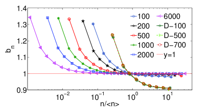
Fig. 7 shows $b_{n}$ vs. $n/\langle n\rangle$ for various system sizes for the SOC BTW model. The behavior is qualitatively similar to that for solar flare intensities, and for stock market volumes. The range of $n$ where $b_{n}$ is close to one increases with system size $L$. The subcritical region occurs for large $n$ as a result of dissipation at the boundaries, which limits the maximum size of $n$. This means that after a large toppling event the system is more likely to undergo a smaller one and $b_{n}<1$. We attempted a finite size scaling analysis, which did not give compelling results. This is consistent with previous results indicating that the SOC BTW model does not obey finite size scaling De Menech et al. (1998); Tebaldi et al. (1999).

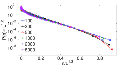
Fig. 8 shows the probability distribution $P(n)$, which has an approximately exponential decay. This differs from the comparable result shown in Fig. 6 for the solar X-ray intensity. Hence, the behaviour exhibited by $b_{x}$ is robust for systems that have markedly different distributions for activity. As shown in Fig. 8, we attempted a finite size data collapse of the distribution of activity, but this collapse shows systematic deviations. However, it is clear that for the distributions the correlation length increases with system size, leading to a broadening distribution of activity in the large $L$ limit for the SOC BTW model.

Figure 8: (color on-line) The probability distribution for activity in the SOC BTW model, $P(n)$. Error bars are smaller than symbol size. The decay is approximately exponential. The best data collapse of the tail of the distribution is obtained by rescaling with $L^{1.2}$. Since the SOC BTW model does not exhibit finite size scaling this rescaling is only for the purpose of plotting all the data together.

Figure 9: (color on-line) Probability distribution function $P(\xi_{n}/n)$ for the SOC BTW model. Error bars are smaller than symbol size. The distribution is shown for $n=15,150,450$, with $L=500$. The system for $n=15$ lies in the supercritical region, while for $n=150$ and $n=450$ it lies in the subcritical region. In all cases the distributions are indistinguishable from Gaussian.

Figure 10: (color on-line) The variance of the random variable $\xi_{n}$, $\sigma^{2}(\xi_{n})/n$ vs. $n$ for three different system sizes. The ratio goes to a constant for large $n$. Hence the variance of $\xi_{n}$ grows as $n$.

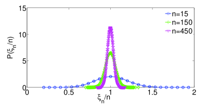
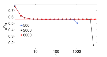
We examined the probability distribution, $P(\xi_{n}/n)$ for various values of $n$. For $n$ sufficiently larger than one, the distribution is well-described by a Gaussian. Fig. 9 shows the distribution function for three values of $n$ in a system of size $L=500$, one in the supercritical regime and two in the subcritical one. Fig. 10 shows that the variance of the random variable $\xi_{n}$ increases linearly with $n$. Gaussian behavior with a variance that grows linearly with $n$ indicates that the activity in the BTW model obeys a central limit theorem: when sampling over prior histories, for each $n$ the activity is the sum of $n$ independent random processes.

IV.2 Dissipative BTW Model

We analyze a BTW model that includes bulk dissipation to test how criticality affects the activity dependent branching ratio. The model is similar to the SOC BTW model except it also includes bulk dissipation Vespignani et al. (1995). When a site topples all its grains are removed from the system with probability $p_{d}$, and with probability $1-p_{d}$ the normal toppling rule applies. Fig. 7 compares the branching ratio for the dissipative BTW model with $p_{d}=10^{-2}$ to the SOC version. It shows that the broad region where $b_{n}$ is approximately equal to one disappears once dissipation is introduced.

IV.3 BTW Model with Periodic Boundary Conditions

We also studied the BTW model with periodic boundary conditions, so that no grains are ever thrown out of the system. As grains are added, an infinite avalanche eventually occurs. We only examine statistics of the infinite avalanche. This corresponds to a fixed energy sandpile, which have been previously studied in Vespignani et al. (2000, 1998); Dickman et al. (1998); Bagnoli et al. (2003). In our analysis, an avalanche that lasts more than $9\times 10^{7}$ parallel update steps is considered to be infinite, and we only collect statistics during the infinite avalanche.

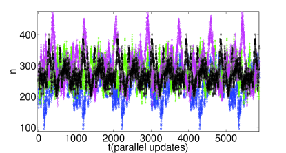
Fig. 11 shows the time series $n_{t}$ for four infinite avalanches during $6000$ time steps. The figure shows that $n_{t}$ is periodic and not ergodic, as was previously noted in e.g. Ref. Bagnoli et al. (2003). For each realization of the infinite avalanche the dynamic range of $n$ is small compared to SOC BTW model. Moreover, the system is sensitive to initial conditions. We tested this sensitivity to initial conditions by starting the lattice empty, or by randomly initializing each site to a value of $0$ or $1$. The initial conditions affects both the period, and the amplitude of oscillations of the infinite sized avalanche. Similar results were also obtained by simply keeping the same initial conditions and changing the seed of the random number generator used. Changing the seed alone was enough to similarly affect the period and amplitude of oscillations. All these results imply that the BTW model with periodic boundary conditions is not ergodic and cannot be compared to the other systems studied here in a meaningful way.

Figure 11: (color on-line) Time series of activity $n_{t}$ for different initial conditions for the BTW model with periodic boundary conditions. This displays different oscillatory behaviour for different initial conditions. In each case a system of size $L=500$ was used.

IV.4 Previous definitions of the branching ratio

The activity dependent branching ratio defined in this paper differs from the average branching ratio measured in de Carvalho and Prado (2000); Christensen et al. (2001). The previously defined ratio was not conditioned on activity but rather defined as the average activity, over all avalanches, resulting from a single toppling. Indeed it was shown that this average branching ratio ${\bar{b}}=1-1/\langle s\rangle$, where $\langle s\rangle$ is the average avalanche size. Hence ${\bar{b}}$ is not an independent quantity, and is always, by definition, less than or equal to one, as long as the average avalanche size is finite. Our activity dependent branching ratio is not restricted to situations where an avalanche can be well-defined or one can identify individual sites for activity. In addition it gives an overall picture for how the system behaves at different levels of activity, unlike the average in Ref. de Carvalho and Prado (2000); Christensen et al. (2001), which sums over all observed levels of activity.

V Discussion and Conclusions

In this paper we introduced an activity dependent branching ratio, $b_{x}$, and use it to analyze different time series, $X_{t}$, arising in physical, economic, and model systems.

We found that stock prices have a branching ratio indistinguishable from unity over for all observed prices. This observation is consistent with the weak efficient market hypothesis. Conversely, stock volume, solar X-ray flux, and the self-organized critical BTW model exhibit supercritical branching ratios for small levels of activity and subcritical ratios for large ones. This indicates a tendency for these systems to return to a characteristic value. This tendency is most pronounced for stock volumes which show a trend consistent with power law with exponent $\simeq 0.69$, for three out of four of the stocks examined. It is not yet clear what separates the Apple stock in our analysis from the other three, or what the source of the apparent scaling is. Solar X-ray flux, and the BTW model both show a broad region where the activity dependent branching ratio $b_{x}\approx 1$. When bulk dissipation is introduced into the BTW model this broad region disappears, supporting our hypothesis that this is a signature of criticality.

The BTW model and solar X-ray flux show this similarity despite having different underlying probability distributions for $X_{t}$. For solar X-ray flux the distribution of flux intensities is consistent with a power law with exponent $\simeq 2.3$, while for the self-organized critical BTW model the distribution of activity $P(n)$ has an approximately exponential decay, with a correlation length that grows with system size.

We also found that the variance in activity $\sigma^{2}(\xi_{n})$ scales linearly with $n$ for the BTW model, and the distribution of subsequent activity is Gaussian at a fixed $n$. This indicates that the BTW model obeys a central limit theorem when sampling over past histories. It remains to be seen if this last result can be derived theoretically.

VI Acknowledgments

We thank P. Grassberger and V. Sood for useful discussions, and M. Baiesi for help with the solar flare data.

References

- Samuelson (1965) P. A. Samuelson, Indust. Manag. Rev. 6, 41 (1965).
- Mandelbrot (1966) B. Mandelbrot, J. Business 39, 242 (1966), ISSN 00219398.
- F. (1989) L. S. F., J. Econ. Lit. 27, 1583 (1989).
- McCauley et al. (2008) J. L. McCauley, K. E. Bassler, and G. H. Gunaratne, Physica A 387, 3916 (2008).
- Fama (1970) E. Fama, J. Finance 25, 383 (1970).
- Farmer and Lo (1999) J. Farmer and A. Lo, PNAS 96, 9991 (1999).
- Lo (2004) A. Lo, J. Portfolio Manage. 30, 15 (2004).
- Lyons and Peres (In preparation) R. Lyons and Y. Peres, Probability on Trees and Networks (Cambridge University Press, In preparation), chap. 5.1, URL http://mypage.iu.edu/~rdlyons/.
- Paczuski et al. (2005) M. Paczuski, S. Boettcher, and M. Baiesi, Phys. Rev. Lett. 95, 181102 (2005).
- de Carvalho and Prado (2000) J. X. de Carvalho and C. P. C. Prado, Phys. Rev. Lett. 84, 4006 (2000).
- Christensen et al. (2001) K. Christensen, D. Hamon, H. J. Jensen, and S. Lise, Phys. Rev. Lett. 87, 039801 (2001).
- (12) URL http://ashkon.com/downloader.html.
- (13) URL http://finance.yahoo.com/q?s=^DJI.
- Mantegna and Stanley (1995) R. Mantegna and H. Stanley, Nature 376, 46 (1995).
- Baiesi et al. (2006) M. Baiesi, M. Paczuski, and A. Stella, Phys. Rev. Lett. 96, 51103 (2006).
- Uritsky et al. (2007) V. Uritsky, M. Paczuski, J. Davila, and S. Jones, Phys. Rev. Lett. 99, 25001 (2007).
- Lu and Hamilton (1991) E. Lu and R. Hamilton, Astrophys. J. 380, 89 (1991).
- Paczuski and Hughes (2004) M. Paczuski and D. Hughes, Physica A 342, 158 (2004).
- Charbonneau et al. (2001) P. Charbonneau, S. McIntosh, H. Liu, and T. Bogdan, Sol. Phys. 203, 321 (2001).
- (20) URL http://spidr.ngdc.noaa.gov/spidr/.
- Bak et al. (1987) P. Bak, C. Tang, and K. Wiesenfeld, Phys. Rev. Lett. 59, 381 (1987).
- Bak et al. (1988) P. Bak, C. Tang, and K. Wiesenfeld, Phys. Rev. A 38, 364 (1988).
- De Menech et al. (1998) M. De Menech, A. L. Stella, and C. Tebaldi, Phys. Rev. E 58, R2677 (1998).
- Tebaldi et al. (1999) C. Tebaldi, M. D. Menech, and A. L. Stella, Phys. Rev. Lett. 83, 3952 (1999).
- Vespignani et al. (1995) A. Vespignani, S. Zapperi, and L. Pietronero, Phys. Rev. E 51, 1711 (1995).
- Vespignani et al. (2000) A. Vespignani, R. Dickman, M. A. Muñoz, and S. Zapperi, Phys. Rev. E 62, 4564 (2000).
- Vespignani et al. (1998) A. Vespignani, R. Dickman, M. A. Muñoz, and S. Zapperi, Phys. Rev. Lett. 81, 5676 (1998).
- Dickman et al. (1998) R. Dickman, A. Vespignani, and S. Zapperi, Phys. Rev. E 57, 5095 (1998).
- Bagnoli et al. (2003) F. Bagnoli, F. Cecconi, A. Flammini, and A. Vespignani, Europhys. Lett. 63, 512 (2003).