Ergodic Considerations in the gravitational potential of the Milky Way

Abstract

A method is proposed for constraining the Galactic gravitational potential from high precision observations of the phase space coordinates of a system of relaxed tracers. The method relies on an “ergodic” assumption that the observations are representative of the state of the system at any other time. The observed coordinates serve as initial conditions for moving the tracers forward in time in an assumed model for the gravitational field. The validity of the model is assessed by the statistical equivalence between the observations and the distribution of tracers at randomly selected times. The applicability of this ergodic method is not restricted by any assumption on the form or symmetry of the potential. However, it requires high recision observations as those that will be obtained from missions like SIM and GAIA.

1 Introduction

Measurements of velocities of cosmological objects are a classic probe of the mass distribution on all scales. It was the motions of individual galaxies in galaxy clusters which first showed that luminous mater contributed only a small fraction to the total mass in clusters Zwicky (1937), implying the existence of dark matter. The combined mass of the Milky Way (or the Galaxy) and M31 is constrained from the observed relative motion between the two galaxies and the requirement that the initial distance between their respective centers of mass vanishes near the Big Bang Kahn & Woltjer (1959). Line-of-sight velocities of other galaxies in the Local Group of galaxies also are used to estimate its mass by the condition of vanishing initial distances Peebles (1989). On scales 10s of Mpcs, peculiar motions (deviations of Hubble flow) of galaxies constrain the global mass density in the Universe (e.g. Nusser, 2008).

Determining the mass distribution in the Milky Way is particularly important. There is ample information on the baryonic content of the Galaxy which could be modeled in detail only if the dark matter distribution is known. The rotation curve of the Galaxy is limited to distances smaller than 20 kpc and does not provide any information on deviations from spherical symmetry of the halo. The mass distribution at larger distances, motions of Galactic satellite galaxies, globular clusters and stars are invoked (e.g. Sakamoto et al., 2003). Constraints on the Galactic mass from these tracers are derived from the condition that the observed speeds of Galactic objects do not exceed the escape velocity. This approach yields only a lower limit and is mostly sensitive to the highest velocity objects. The vast majority of the sample objects play no role in deriving the mass limit. Alternatively, one could adopt a Bayesian likelihood formalism in which the phase space distribution function is assumed to follow certain form which could be matched with the observations to probe the Galactic potential field (e.g. Little & Tremaine, 1987; Kochanek, 1996; Wilkinson & Evans, 1999) .

Proper motions, resulting from velocities perpendicular to the line-of-sight, are currently measured only for nearby tracers (e.g. Sakamoto et al., 2003). Therefore, most current mass estimates rely on the measured line-of-sight motions of individual components. During the next few years, accurate proper motions for a large sample of Galactic tracers are expected to be measured by the space missions Global Astrometry Interferometer for Astrophysics (GAIA) Lindegren & Perryman (1996) and Space Interferometry Mission (SIM) Unwin et al. (2008). Even accurate phase space information require additional assumptions in order to constrain the Gravitational potential . We present here a general method which relies on high precision measurements of positions and velocities of tracers. The method assumes that the tracers have reached an equilibrium state in the Galactic gravitational field.

2 The method

The expected precision of future data of proper motions, radial velocities and distances will allow an accurate determination of the orbits of tracers in a given Galactic gravitational field. This motivates the “ergodic” method which constrains the gravitational potential by the hypothesis that the state of a dynamically relaxed system of tracers at any time is statistically representative of that system at any other time. The method is described as follows.

1. assume a model for the gravitational potential field $\Psi(r,\alpha,\beta\dots)$ where $\alpha$, $\beta$ etc are free parameters.

2. for a given choice of free parameters, use the observations as initial conditions at time $t={t_{{}_{0}}}$ to advance the particles (tracers), in the gravitational field $\Psi$, for sufficiently long time.

3. select snapshots of the particle distribution at times $t>{t_{{}_{0}}}$

4. compare between statistical measures of the particle distributions in the observed data ($t={t_{{}_{0}}}$) and in the snapshots ($t>{t_{{}_{0}}}$). If necessary, repeat (ii)-(iv) with a different choice of free parameters until a reasonable agreement is reached.

We work here with four statistical measures. The first is the $N$ statistic computed as follows. Consider all snapshots (at $t>{t_{{}_{0}}}$) corresponding to an assumed value of $\alpha$. For a snapshot $s$, we compute $N_{\rm s}$ defined as the number of particles with Galactic distances that are larger than the respective observed distances. We define the statistic $N$ as $N=<N_{\rm s}>$, the average of $N_{\rm s}$ over all snapshots. We further define $\sigma=<(N_{\rm s}-N)^{2}>^{1/2}$, as the r.m.s. scatter in $N_{\rm s}$. In the limit of a large number of tracers, $n$, the limits $N_{\rm s}=n/2$ and $N=n/2$ are approached for the correct model. The second is the distribution function of the Galactic distances, ${r}$, of tracers, i.e. the density of tracers as a function of distance. The third measure is distribution function of

$$\xi=\frac{{r}-{r_{{}_{\rm min}}}}{{r_{{}_{\rm max}}}-{r_{{}_{\rm min}}}}\;,$$ (1)

computed from the Galactic distances, ${r}$, of particles in each snapshot. The pericenter, ${r_{{}_{\rm min}}}$, and apocenter, ${r_{{}_{\rm max}}}$, of each particle is computed from the numerically integrated orbits. The distributions of $r$ and $\xi$ computed from the observations given at ${t_{{}_{0}}}$ should be statistically equivalent to the respective distributions in any snapshot at $t>{t_{{}_{0}}}$ if the system is evolved to $t>{t_{{}_{0}}}$ using a gravitational potential which is a reasonable approximation to the true potential field. Significant differences between the initial and later distributions should appear if the integration at $t>{t_{{}_{0}}}$ is performed with sufficient deviations from the original gravitational potential. To see this consider the simple case of particles executing circular motions in the gravitational field of a point mass, $M_{0}$. Now let us use a snapshot of the motion of this system at time $t={t_{{}_{0}}}$ as initial conditions to move the particles forward in time in the field of the point mass $M\ll M_{0}$. The pericenters, ${r_{{}_{\rm min}}}$, of orbits obtained with $M$ will equal the initial distances so that $\xi=0$ for all particles at time ${t_{{}_{0}}}$. However, the distances at a randomly selected later time $t\gg{t_{{}_{0}}}$ span the range ${r_{{}_{\rm min}}}$ to ${r_{{}_{\rm max}}}$, yielding $\xi$ from 0 to 1 (the $\xi$ distribution peaks at the end points where the radial velocities are zero). Therefore, $M\ll M_{0}$ could be rejected by the gross mismatch between the $\xi$ distributions at the initial time ${t_{{}_{0}}}$ and at $t\gg{t_{{}_{0}}}$. Similar arguments apply for the distribution function of $r$.

The fourth statistic is based on the virial relation between the total kinetic energy (per unit mass) $T=\sum\dot{\bf r}^{2}/2$ and a term $W$ related to the gravitational force field. In order to derive the explicit relation, we perform a scalar multiplication of the radius vecor, ${\bf r}$ of each particles with the corresponding equation of motion ${\rm d}{\bf v}/{\rm d}t=-{\mathbf{\nabla}}\Psi$. Summation over all particles and time averaging gives

$$2\overline{T}=\overline{W}\;,\quad{\rm where}\quad W\equiv-\sum_{tracers}{\bf r}\cdot{\bf\nabla}\Psi\;,$$ (2)

and the over-lines denote time averaging. Therefore, as our fourth statistic we consider the ratio $|W|/2T$ computed directly from the observations for an assumed form of $\Psi$. Since the virial relation applies to time average quantity, this statistic, computed at a single time, is expected to deviate from unity for a finite number of particles. Therefore, although the statistic could be computed without evolving the particles in time, snapshots at later times will be used to compute the scatter in the statistic. This ratio differs from the other statistics in that it directly involves the observed velocities. It is only sensitive to the force field at the observed positions of the tracers. i

3 Tests

Thorough tests of the performance of the method should take into account the details of future observations. Although this is necessary in order to provide reliable error estimates, the task seems futile at this early stage. The preliminary tests presented here aim at demonstrating the ability of the method to yield significant constraints on a one parameter family for the form of $\Psi$ as given below. We test the method using catalogs of mock data of dynamically relaxed tracers. The system is assumed to exist in a galaxy made of a spherical dark matter halo and a baryonic disk, neglecting the gravitational effects of a bulge. The gravitational potential of the halo is taken as Sakamoto et al. (2003); Dinescu et al. (1999)

$$\Psi_{{}_{\rm halo}}=\left\{\begin{array}[]{ll}{v_{{}_{\rm h}}}^{2}\ln\left[1+(r/d)^{2}\right]-\Psi_{0}\;,&{\rm for}\quad r<{r_{{}_{\rm cut}}}\\ -2\frac{{v_{{}_{\rm h}}}^{2}}{r}\frac{{r_{{}_{\rm cut}}}^{3}}{{r_{{}_{\rm cut}}}^{2}+d^{2}}\;,&{\rm otherwise}\;,\end{array}\right.$$ (3)

where $\Psi_{0}$ is a constant ensuring the continuity of the force field per unit mass, $-{\bf\nabla}\Psi_{{}_{\rm halo}}$, at $r={r_{{}_{\rm cut}}}$. We take ${v_{{}_{\rm h}}}=128\mbox{km\,s${}^{-1}$}$, $d=12{\;{\rm kpc}}$ and ${r_{{}_{\rm cut}}}=170{\;{\rm kpc}}$ as in Sakamoto et al. (2003). For the potential of the disk we work with the form (Miyamoto & Nagai 1975),

$${\Psi_{{}_{\rm disk}}}=\frac{-G{M_{{}_{\rm disk}}}}{\sqrt{R^{2}+\left(a+\sqrt{z^{2}+b^{2}}\right)^{2}}}\;,$$ (4)

where $d=12{\;{\rm kpc}}$, ${M_{{}_{\rm disk}}}=10^{11}M_{\odot}$, $a=6.5{\;{\rm kpc}}$ and $b=0.26{\;{\rm kpc}}$ Dinescu et al. (1999). The mock observations are generated as follows. Particles are placed in the halo by a random Poisson sampling of an underling number density $n(r)\propto 1/r^{2}$. The corresponding velocities are selected randomly from a gaussian distribution with zero mean and a r.m.s proportional to the local escape speed such that the total kinetic energy is half the absolute value of the potential energy, as implied by the virial theorem. The equations of motion of the system are then solved numerically for $10\rm\;Gyrs$ to ensure dynamical relaxation in the gravitational field given in Eqs. 3 & 4. Outputs of particle positions and velocities obtained from this procedure are then identified as the mock catalog to be used for testing the method. As our model gravitational potential we use the forms in Eqs. 3 & 4 but with ${M_{{}_{\rm disk}}}$ and ${v_{{}_{\rm h}}}^{2}$ scaled by a factor $\alpha$ according to $({M_{{}_{\rm disk}}},{v_{{}_{\rm h}}}^{2})\rightarrow(\alpha{M_{{}_{\rm disk}}},\alpha{v_{{}_{\rm h}}}^{2})$. The tests are performed for one free parameter, $\alpha$. Following the scheme above, the mock catalog provide the initial conditions at time ${t_{{}_{0}}}$ for moving the particles for another $10\rm\;Gyrs$ for an assumed value of $\alpha$. Snapshots of particle positions are then tabulated at 1000 uniformly distributed time steps between ${t_{{}_{0}}}$ and ${t_{{}_{0}}}+10\;\rm Gyrs$. This is done for 17 values of $\alpha$ spanning the range $0.7-1.5$ linearly. The tests will demonstrate that the method is able to recover the correct value, $\alpha=1$, within an acceptable uncertainty.

3.1 Tests with zero measurement errors

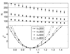
Figure 1: Left: The statistic $N$ as a function of $\alpha$ shown as the filled circles with error-bars representing the r.m.s scatter, $\sigma$ (see text). Three values of the number of tracers are considered, $n=200$, 300 and 500 and the three horizontal lines indicate corresponding limiting values $N=n/2$. Right: Curves of $\chi^{2}=(N-n/2)^{2}/\sigma^{2}$ as a function of $\alpha$ for several values of $n$, as indicated in the figure.

We start with the statistic $N$ computed from snapshots corresponding to an assumed $\alpha$. The filled circles in the left panel of Fig. 1 show $N$ as a function of $\alpha$, for three values of the number of tracers, $n=200$, 300 and 500. The error-bars represent the r.m.s scatter, $\sigma$. The horizontal solid lines indicate the limit, $N=n/2$, corresponding to the three values of $n$. For $\alpha$ close to unity, $N$ is indeed near $n/2$ even for $n=200$. For better quantification of these results we plot in the right panel the quantity $\chi^{2}(\alpha)=(N-n/2)^{2}/\sigma^{2}$. Curves of $\chi^{2}$ become narrower as $n$ is increased, but already with $n=200$ significant constraints on $\alpha$ could be derived. Note that $<(N_{\rm s}-n/2)^{2}>/\sigma^{2}=1+\chi^{2}$ so that $\chi^{2}=3$ correspond to a $2\sigma$ deviation of $N_{\rm s}$. We see that $n=200$ already constrains $\alpha$ to better than 25% at the $2\sigma$ level.

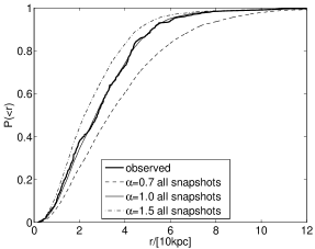
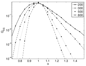
Figure 2: Left: CPDFs of the distances for $300$ tracers. The thick line shows $P(<r)$ computed from the observed “distances: at $t={t_{{}_{0}}}$, while the three smooth thin lines represent the model CPDF ${P_{{}_{\rm m}}}(<r)$ for three values of $\alpha$, as indicated in the figure. Right: The confidence level ${Q_{{}_{\rm KS}}}$ that $P(<r)$ and ${P_{{}_{\rm m}}}(<r)$ represent the same distribution, as a function of $\alpha$.

We now turn to the distribution function of $r$ and $\xi$ as described in §2. We define the cumulative distribution function (hereafter CPDF), $P(<y_{1})$, at any time, as the fraction of particles having $y<y_{1}$, where $y$ is either $r$ or $\xi$. Hereafter, we will treat the CPDF obtained from the ensemble of 1000 snapshots as the underlying actual model CPDF and denote it by ${P_{{}_{\rm m}}}$. In the left panel of Fig. 2 we illustrate the differences between the various CPDFs obtained with $300$ tracers. The thick solid curve is the CPDF $P(<r)$ obtained from the “observed” positions in the mock catalog, while the dashed, thin solid, and dot-dashed lines correspond to ${P_{{}_{\rm m}}}(<r)$ for $\alpha=0.7$, 1, and 1.5, respectively. The CPDF ${P_{{}_{\rm m}}}(<r)$ is sensitive to $\alpha$. The value $\alpha=0.7$ broadens the distribution of particles towards larger radii, relative to the “observed” CPDF, while $\alpha=1.5$ concentrates the particles nearer to the center. The CPDF ${P_{{}_{\rm m}}}(<r)$ for $\alpha=1$ (smooth thin solid line) seems consistent with the “observed” CPDF (thick solid). To quantify the differences between model and observed “observed” CPDFs, we compute the Kolmogorov-Smirnov (KS) “distance” $D_{\alpha}=\sup_{{}_{r}}|{P_{{}_{\rm m}}}(<r)-P(<r)|$ where the dependence on $\alpha$ is only through ${P_{{}_{\rm m}}}(<r)$. Given $D_{\alpha}$ and the number of tracers, $n$, we compute the significance level, $Q_{{}_{\rm KS}}$, of the hypothesis that $P(<r)$ and ${P_{{}_{\rm m}}}(<r)$ represent the same distribution. In the right panel of Fig. 2, we plot $Q_{{}_{\rm KS}}$ as a function of $\alpha$ for $n=200$, 300, 500 and 800, as indicated in the figure. All curves peak near the value, $\alpha=1$. The only uncertainty in determining $\alpha$ is due to the finite number of tracers, hence the peaks are narrower for larger $n$. For all values of $n$ considered here, the choice $\alpha=1$ is never “rejected” at more than the $32\%$ confidence level (i.e. ${Q_{{}_{\rm KS}}}<0.32$), equivalent to a $1\sigma$ level for a normal distribution. Thus the method produces unbiased estimates of $\alpha$ within the $1\sigma$ errors. For $n=200$, deviations of $\alpha$ larger than $\sim 30\%$ from unity are rejected at more than the $2\sigma$ level (i.e. ${Q_{{}_{\rm KS}}}<0.045$).

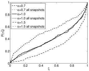
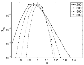
Figure 3: Left: CPDFs of $\xi$ for 300 tracers. The three thick lines represent “observed” $P(<\xi)$ computed with ${r_{{}_{\rm min}}}$ and ${r_{{}_{\rm max}}}$ corresponding to $\alpha=0.7$, 1 and $1.5$, as indicated in the figure. The nearly overlapping three smooth thin lines represent the model ${P_{{}_{\rm m}}}(<\xi)$ corresponding to the same choice of $\alpha$ values. Right: The confidence level ${Q_{{}_{\rm KS}}}$ as a function of $\alpha$.

We now explore the CPDFs of $\xi$. The CPDF $P(<\xi)$ computed from the “observed” particle positions in the mock catalog depend on the assumed $\alpha$ through the pericenters, ${r_{{}_{\rm min}}}$, and apocenters, ${r_{{}_{\rm max}}}$, of the orbits. This is in contrast to the observed $P(<r)$ which is completely independent of $\alpha$. The three thick lines in the left panel of Fig. 3 are the CPDFs $P(<\xi)$, computed from the “observed” positions of 300 particles, for $\alpha=0.7$, 1 and 1.5, as indicated in the figure. The three nearly overlapping thin dashed, thin solid and thin dot-dashed lines show ${P_{{}_{\rm m}}}(<\xi)$, respectively, for these three $\alpha$ values. The dependence of ${P_{{}_{\rm m}}}(<\xi)$ on $\alpha$ is very weak, in contrast to ${P_{{}_{\rm m}}}(<r)$ which is very sensitive to the assumed $\alpha$. This weak dependence is not entirely unexpected since $\xi$ eliminate the overall length scale of the problem. For $\alpha=0.7$, the difference between ${P_{{}_{\rm m}}}(<\xi)$ (thin dashed line) and $P(<\xi)$ (thick dashed) implies that most of the “observed” positions are closer to the pericenters than the positions in the snapshots. For $\alpha=1.5$ (thin and thick dot-dashed lines), the “observed” positions are closer to the apocenters than the positions in the snapshots. For the correct value $\alpha=1$, the distributions ${P_{{}_{\rm m}}}(<\xi)$ (thin solid) and $P(<\xi)$ (thick solid) appear to be consistent. To test whether the difference between ${P_{{}_{\rm m}}}(<\xi)$ and $P(<\xi)$ is large enough to rule an assumed $\alpha$ we show in Fig. 3 the corresponding quantity $Q_{{}_{\rm KS}}$ as a function of $\alpha$ for $n=200$, 300, 500 and 800, as indicated in the figure. As is the case for the CPDFs of $r$, the value $\alpha=1$ is never “rejected” at more than the $1\sigma$ level. All curves are narrower than the corresponding curves in the right panel of Fig. 2, implying a better ability to constrain $\alpha$ with the distribution of $\xi$ than of $r$. For $n=200$, deviations of more than $20\%$ from $\alpha=1$ are rejected at more than the $2\sigma$ (${Q_{{}_{\rm KS}}}<0.045$) level. For a given confidence level, the range of $\alpha$ (i.e. confidence interval) constrained by the distribution of $\xi$ is narrower by a factor of 2 than the range constrained by distribution of $r$.

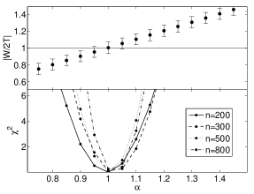
Figure 4: Left: The filled circles show the ratio, $|W/2T|$, versus $\alpha$ from the observed distances and velocities of 200 mock tracers at ${t_{{}_{0}}}$. The error-bars show the r.m.s. scatter, $\sigma$, computed from snapshots at $t>{t_{{}_{0}}}$. The horizontal line indicates the virial theorem value for $\overline{W}/2\overline{T}$. Right: The quantity $\chi^{2}=[|W/2T|-1]^{2}/\sigma^{2}$ versus $\alpha$.

The statistic $|W/2T|$ computed form the mock observations with $n=200$ is presented as a function of $\alpha$ by the filled circles in the left panel of Fig. 4. Here $T$ is computed with the “observed” velocities and the dependence on $\alpha$ is entirely due to the $W$ term (see Eq. 2). For each $\alpha$, the error-bars show the r.m.s scatter, $\tilde{\sigma}$, of $|W/2T|$ estimated from snapshots generated with that $\alpha$. As a consistency check we confirm that the departure from unity of the ratio $\overline{W}/2\overline{T}$, obtained by averaging $W$ and $T$ over the snapshots, is completely insignificant compared to the $1\sigma$ scatter. The deviation from unity of $|W/2T|$ computed from the mock observations is shown in the right panel of the Fig. 4 as $\chi^{2}=[|W/2T|-1]^{2}/{\tilde{\sigma}}^{2}$. For $n=200$, this statistic constrains $\alpha$ to better than $15\%$ at the $2\sigma$ confidence level. This is better than the $N$ statistic which constrains $\alpha$ to better than $25\%$ at the same confidence level. It also fares slightly better than the $\xi$ distribution.

3.2 Effect of measurement errors

So far we have assumed zero errors in the phase space coordinates. We present here only partial tests of the method when applied on noisy data. The amplitude of the errors depends on the distance of tracers from an observer at the solar position rather than the galactocentric distances. We assign a 15% error in the distance of a tracer from an observer present in the Galactic disk at 8$\rm kpc$ from the Galactic center. For GAIA a 10% parallax distance error corresponds to objects of 15 mag at $10\rm kpc$ from the observer. Errors in parallax distances scale quadratically with true distance and become very large at distances of tens of kpcs even for GAIA and SIM. Here we assume that distances of far away tracers are determined by other means so that a linear scaling of the errors is maintained. We also perturb the radial velocities and proper motions with errors that scale linearly with distance. The amplitude velocity errors is assumed equal in all three directions and is normalized to a r.m.s value of $10\mbox{km\,s${}^{-1}$}$ at a distance of $20{\;{\rm kpc}}$. For comparison, at 15 mag, GAIA after 5 years of operation will provide radial motions within an accuracy of $10-15\mbox{km\,s${}^{-1}$}$ and proper motions within an accuracy of $1\mbox{km\,s${}^{-1}$}$ at a $20{\;{\rm kpc}}$.

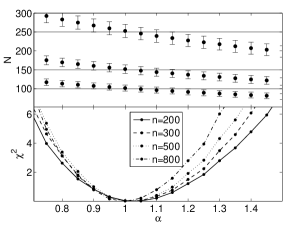
Figure 5: The same as Fig. 1, but with degraded mock observations by random errors as described in the text.

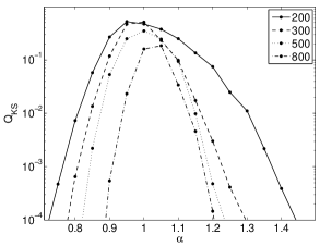
Figure 6: The same as the right panel of Fig. 3, but with degraded mock observations.

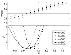
Figure 7: The same as Fig. 4, but with degraded mock observations.

We do not show results for $P(<r)$ computed with errors included as it yields less significant constraints than the remaining statistics. The results for $N$ and $\xi$ are shown in Fig. 5 and Fig. 6, respectively. For $n=200$ and 300, there is little difference between the curves of $\chi^{2}$ and ${Q_{{}_{\rm KS}}}$ in these figures and in Figs. 1 & 3 corresponding to zero errors. For larger $n$ the effect of the errors is more pronounced, especially in ${Q_{{}_{\rm KS}}}$. The reason for this behavior is that sampling errors resulting from the finite number of tracers are dominant over measurement errors for the smaller values of $n$. As $n$ increases, measurement errors become more pronounced resulting in the significant reduction of the value of ${Q_{{}_{\rm KS}}}$ at $\alpha=1$ for $n=800$. The $N$ statistic seems to be more resilient to measurement errors than the $\xi$ distribution. The virial ratio $|W/2T|$ computed with noisy mock data is shown in Fig. 7 with the same notation as Fig. 4 corresponding to results with zero measurement errors. In computing $T$, the mean of non-vanishing quadratic terms due to velocity errors have been removed. Measurement errors seem to affect the ratio more than the other statistics. Still, this ratio constraints $\alpha$ slightly better than the other statistics.

Overall, measurement errors of the amplitude we consider here have not degraded the ability of the method at constraining $\alpha$. Therefore, the method does not require unrealistically accurate data.

3.3 Effect of gradually growing disk

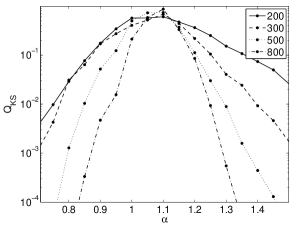
Figure 8: The confidence level ${Q_{{}_{\rm KS}}}$ as a function of $\alpha$, assuming a gradually growing disk (see text).

The method assumes a constant gravitational potential. However, the Galactic disk may have grown substantially in the last 8Gyr or so. Here we check whether this gradual growth seriously hampers the application of the method. We solve for the orbits of tracers assuming that the mass distribution of the disk grows like $t^{0.3}$. The method is then applied to the resultant distribution of tracers in phase space assuming a constant disk. In Fig. 8 we show the confidence level ${Q_{{}_{\rm KS}}}$ as a function of $\alpha$ where in this case the mass in the disk is assumed to be known and $\alpha$ describes the ratio of the assumed ${v_{{}_{\rm h}}}$ to the actual value.

4 Concluding Remarks

The ergodic method presented here requires a parametric functional form for the Gravitational potential, but does not impose any special symmetry on the mass distribution. The method assumes that the observations of a class of tracers are spatially complete. Tracers with observed distances smaller than $d_{0}$, could be present beyond $d_{0}$ in snapshots at later times. Therefore, Observational selection against tracers at distances $>d_{0}$ will make the statistical comparison between observations and snapshots at later times extremely difficult. The completeness is not too demanding a condition for tracers like globular clusters and Galactic satellites for which future observations should be accurate enough for quite large Galactic distances.

We have presented only partial testing of the method, with only a one parameter family for the form of the Galactic potential. Method is able to constrain the parameter to a good accuracy with measurements errors that are even larger than those expected to be achieved by future data. The tests show that the method could provide unbiased constraints on the Gravitational potential, but a more elaborate testing which includes a more realistic treatment of the errors should be done. Observations will likely assign distance and velocity measurement errors to tracers on an individual basis. Therefore, random errors and systematic biases tailored to the specific sample of tracers used by the method could be determined robustly.

The accuracy of the method is mainly limited by the number of tracers. The most obvious tracers are globular clusters and Galactic satellites. Our Galaxy includes 158 known globular clusters, and 23 known satellites (e.g. Simon & Geha, 2007). Distance measurements of RR Lyrae stars from their period-luminosity relation will be greatly improved by GAIA and SIM calibration of the zero point using a nearby sample of these stars. Therefore, luminous halo RR Lyrae stars could significantly enlarge the sample of tracers.

The method requires a system of tracers in dynamical equilibrium in the current Galactic potential. A pre-requist for dynamical equilibrium is that any recent changes in the Galactic potential must have occurred on a time scale longer that the dynamical time of the system of tracers. Spectroscopic studies stars in the Galaxy do not present evidence for substantial mergers in the last 8Gyr Gilmore et al. (2002); Helmi et al. (2006), implying a nearly static gravitational potential. We have demonstrated that adiabatic growth of the Galactic disk is not expected to pose a problem for the implementation of the method. The effect of any deviation from that should be modeled.

One issue which is exclusive to using disk stars as tracers is the effect of transient perturbations on the dynamics of those stars (e.g. Famaey et al., 2005; Quillen, 2003). However, the transient effects cause velocity perturbations at the level of  10 km/s which is much smaller that the total velocities of tracers. Observational uncertainties are larger than that and do not seem to cause significant biases in the results as indicated by the tests described above. Another issue to be considered is halo substructure which, in principle, could act as a stochastic component in the gravitational potential. Such a component is extremely difficult to model in the method proposed here. We offer the following argument demonstrating that substructure should not have an important effect on the long term dynamics of tracers. In the limit of fast encounters, a tracer passing a substructure at distance $b$ will change its velocity by $V_{1}\approx g(b)b/V$ where $V$ is the relative velocity and $g\approx GM/b^{2}$ is the gravitational force field of the substructure assuming that $b$ is larger than its tidal radius. Performing the usual summing in quadratures over encounters occurring in one orbital time we get that the r.m.s change $<V_{1}^{2}>^{1/2}\approx M\sqrt{\bar{n}R}/V$ where $\bar{n}$ is the number density of substructures and $R$ is the distance travelled by the tracer in one orbital time. Taking $V^{2}=GM_{{}_{\rm MW}}(R)/R$ with $M_{{}_{\rm MW}}(R)$ the mass of the Galactic halo within radius $R$, we get the condition $\sim M_{{}_{\rm MW}}\sqrt{\bar{n}R^{3}}>M_{{}_{\rm MW}}$ for having $<V_{1}^{2}>^{1/2}\sim V$. This means that neither single encounters nor collective stochastic effects can dominate the long term evolution of tracers even if the fraction of mass in substructures is large which is contrary to recent simulations (e.g. Colombi, 2008) which show that the smooth component greatly dominates the mass of Galactic size halos.

When details of future data from SIM and GAIA become available, all robust information about the distribution of baryons in the Galaxy should be used (e.g. Robin et al., 2003) in order to place tight constraints on the Galactic dark matter. The validity of the method should be tested with mock data that match the observations as much as possible and with the best possible available Galactic models.

5 Acknowledgments

The author wishes to thank an anonymous referee for comments which helped improve the paper. This work is supported by the German-Israeli Foundation for Research and Development and by the Asher Space Research Institute. This research was supported by S. Langberg Research Fund.

References

- Colombi (2008) Colombi, S. 2008, Nature, 456, 44
- Dinescu et al. (1999) Dinescu, D. I., Girard, T. M., & van Altena, W. F. 1999, AJ, 117, 1792
- Famaey et al. (2005) Famaey, B., Jorissen, A., Luri, X., Mayor, M., Udry, S., Dejonghe, H., & Turon, C. 2005, A&A, 430, 165
- Gilmore et al. (2002) Gilmore, G., Wyse, R. F. G., & Norris, J. E. 2002, ApJ, 574, L39
- Helmi et al. (2006) Helmi, A., Navarro, J. F., Nordström, B., Holmberg, J., Abadi, M. G., & Steinmetz, M. 2006, MNRAS, 365, 1309
- Kahn & Woltjer (1959) Kahn, F. D., & Woltjer, L. 1959, ApJ, 130, 705
- Kochanek (1996) Kochanek, C. S. 1996, ApJ, 457, 228
- Lindegren & Perryman (1996) Lindegren, L., & Perryman, M. A. C. 1996, A&AS, 116, 579
- Little & Tremaine (1987) Little, B., & Tremaine, S. 1987, ApJ, 320, 493
- Nusser (2008) Nusser, A. 2008, MNRAS, 384, 343
- Peebles (1989) Peebles, P. J. E. 1989, ApJ, 344, L53
- Quillen (2003) Quillen, A. C. 2003, AJ, 125, 785
- Robin et al. (2003) Robin, A. C., Reylé, C., Derrière, S., & Picaud, S. 2003, A&A, 409, 523
- Sakamoto et al. (2003) Sakamoto, T., Chiba, M., & Beers, T. C. 2003, A&A, 397, 899
- Simon & Geha (2007) Simon, J. D., & Geha, M. 2007, ApJ, 670, 313
- Unwin et al. (2008) Unwin, S. C., Shao, M., Tanner, A. M., Allen, R. J., Beichman, C. A., Boboltz, D., Catanzarite, J. H., Chaboyer, B. C., Ciardi, D. R., Edberg, S. J., Fey, A. L., Fischer, D. A., Gelino, C. R., Gould, A. P., Grillmair, C., Henry, T. J., Johnston, K. V., Johnston, K. J., Jones, D. L., Kulkarni, S. R., Law, N. M., Majewski, S. R., Makarov, V. V., Marcy, G. W., Meier, D. L., Olling, R. P., Pan, X., Patterson, R. J., Pitesky, J. E., Quirrenbach, A., Shaklan, S. B., Shaya, E. J., Strigari, L. E., Tomsick, J. A., Wehrle, A. E., & Worthey, G. 2008, PASP, 120, 38
- Wilkinson & Evans (1999) Wilkinson, M. I., & Evans, N. W. 1999, MNRAS, 310, 645
- Zwicky (1937) Zwicky, F. 1937, ApJ, 86, 217