Direct observation of current in type I ELM filaments on ASDEX Upgrade

Abstract

Magnetically confined plasmas are often subject to relaxation oscillations accompanied by large transport events. This is particularly the case for the high confinement regime of tokamaks where these events are termed edge localized modes (ELMs). They result in the temporary breakdown of the high confinement and lead to high power loads on plasma facing components. Present theories of ELM generation rely on a combined effect of edge current and the edge pressure gradients which result in intermediate mode number ($n\cong 10-15$) structures (filaments) localized in the perpendicular plane and extended along the field line. It is shown here by detailed localized measurements of the magnetic field perturbation associated to an individual type I ELM filament that these filaments carry a substantial current.

Edge localised modes (ELMs) are short (ms) breakdowns of the high confinement regime (H-mode), which is envisaged to be used in power producing tokamaks. Due to the high power fluxes associated, the presence of ELMs poses demands on the design of plasma facing components, that are hard to meet. Thus understanding, with the aim of controlling, ELM events is one of the foremost priorities in fusion research. Moreover, apart from the interest for fusion oriented plasmas, the interest in ELM physics is enhanced by some fascinating analogies with sporadic explosive events as observed for example in solar flares Fundamenski et al. (2007) or in magnetic substorms Lui (2000).

ELMs are at present thought to originate from a combination of current and pressure gradient driven MHD modes Snyder et al. (2005), and are known to result in a medium number ($n\approx 10-15$) of structures Kirk et al. (2006a); Fenstermacher et al. (2005); Herrmann et al. (2007); Kirk et al. (2006b), localised in the perpendicular plane and extended along the magnetic field. These filaments travel through the Scrape Off Layer (SOL) and have been measured using Langmuir probes on various machines, see e.g. Leonard et al. (2006), and observed through high speed cameras Kirk et al. (2006b) or Gas Puff Imaging diagnostic R Maqueda and R Maingi and NSTX team (2009). In this letter we present results of direct measurements of all three components of the magnetic field perturbations associated to ELM filament structures in the SOL together with an estimate of the current carried by filaments.

Magnetic fluctuations associated with ELMs are usually believed to originate from MHD activity. Measurements of the magnetic activity have previously been performed using magnetic pickup coils close to the vessel wall Kirk et al. (2006b); Takahashi et al. (2008) or on insertable probes Herrmann et al. (2008). These measurements generally take place far from the filaments in comparison to their radial extent. This makes it difficult to observe the magnetic perturbation going along with individual filaments and to examine the magnetic fine structure of the ELMs. Both would result in important information such as the excursion of magnetic field lines from their equilibrium position and if the ELMs are associated with reconnection events Fundamenski et al. (2007) .

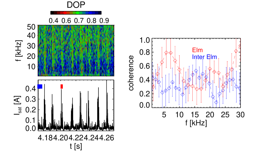
Figure 1: Top: Degree of Polarization (DOP) analysis as a function of time and frequency. Bottom: Ion saturation current (I_sat). Right: Coherence between I_sat and $b_{p}$ computed in the ELM and inter-ELM phases. The time intervals are shown in the bottom panel with colored boxes.

Here we report on measurements of type I ELMs carried out at ASDEX Upgrade (AUG) tokamak by means of a newly constructed probe head described in detail elsewhere Ionita et al. (2009). The probe head consists of a cylindrical graphite case (⌀=60 mm) which holds six graphite pins. One of the tips measured the ion saturation current, one tip was swept, whereas all the others had been kept floating. Inside the case, 20 mm behind the front side, a magnetic sensor measuring the time derivative of the three components of the magnetic field is mounted. The sensor has a measured bandwidth of 1 MHz. A similar probe with combined electrostatic and magnetic signals has already been used in AUG Herrmann et al. (2008), but with a wider magnetic coil and a larger radial separation between electrostatic and magnetic sensors. The probe head, mounted on the fast reciprocating midplane manipulator, is inserted from the low field side of the torus for 100 ms 12 mm inside the limiter position. The data have been obtained in type-I ELMy plasma discharges (# 23158,23159,23160,23161,23163) with a toroidal magnetic field of -2.5 T, 0.8 MA of plasma current, 6.5 $\times 10^{19}$ m^-3 central electron density and a $q_{95}$ value of 5.2.

During the analysis we have used the ion saturation current to infer the passing of a type-I ELM filament structure in front of the probe, as done for example in Endler et al. (2005).

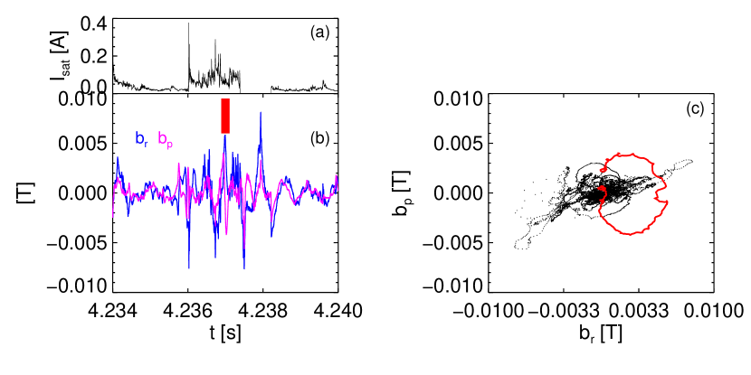
Figure 2: (a)Ion saturation current (b) Poloidal and radial component of the magnetic field. The red box highlights the time interval when the two components change their phase relation. (c) Hodogram of the radial/poloidal magnetic field component. The closed loop in red refers to the time intervals highlighted in panel (a,b).

In analyzing the ELM events we employ the idea that the magnetic signal during the ELM can be separated into different frequency components. Higher frequencies, above few hundred kHz, we presume to be generated mostly by Alfvénic activity or high frequency turbulence. These are not considered in the present analysis, also because of the frequency cut-off by the graphite shielding Ionita et al. (2009). Additional MHD activity will still be present in the signal at frequencies below 20 kHz, but during ELM filaments most of the signal is presumed to originate from slowly varying currents convected with the filaments. This is justified by the so-called Degree of Polarization (DOP) analysis Samson and Olson (1980); *Santolik:2003p3492, which is a test for a plane wave ansatz, quantifying how well the relation $\mathbf{k}\cdot\mathbf{B}=0$ is satisfied. It is based on the evaluation and diagonalization of the spectral matrix $S=\langle B_{i}^{*}B_{j}\rangle$, calculated in Fourier space. The DOP represents a measure to determine whether $S$ represents a pure state quantifying how much one single eigenvector approximates the state. A high value of DOP implies that the fluctuations considered are coherent over several wavelengths, and thus the method can be used to distinguish between propagating modes and coherent localized fluctuations. Figure 1, panel (a), shows the results of DOP analysis as a function of frequency and time. The temporal evolution of the ion saturation current is depicted in the lower panel. A sudden drop in the DOP is observed in correspondance with a steep increase of $I_{sat}$ signals: this implies that the magnetic field fluctuations during an ELM can be better represented by coherent structures than by plane wavepackets.

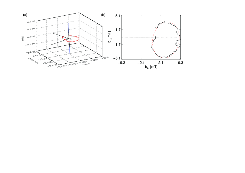
Figure 3: (a)Trajectory of ELM filament associated magnetic field excursions in all three spatial directions. The direction of minimum variance is shown (black line) together with the direction of the equilibrium field (blue line). (b) Hodogram of the magnetic perturbation associated with ELM current filament reconstructed in the maximum variance plane. The red line shows the elliptical fit.

A coherence analysis between the ion saturation current and the poloidal component of the magnetic field (Fig. 1 (c)) reveals an increase of coherence between the two signals during the ELM activity. A closer look on the behavior of magnetic fluctuations associated to an ELM event is shown in Figure 2 (b). When the magnetic fluctuation amplitude increases, the radial and poloidal components ($b_{r}$ and $b_{p}$ ) change their phase relation as highlighted by the color box. We now consider the hodogram of the perpendicular magnetic perturbation (Fig. 2 (c)), i.e. the magnetic field perturbation trajectory in the $b_{r}-b_{p}$ plane, during the passing of the ELM. Here one closed orbit corresponds to the time interval marked in Figure 2 b. Closed loops are compatible with the passing of current filaments in front of the probe. Outside the ELM, the magnetic field perturbation exhibits an almost linear polarization in the perpendicular plane. This shows clearly that magnetic activity in between ELMs (wavelike) differs qualitatively from the magnetic perturbation during an ELM, which seems to be due to the motion of current filaments.

The measurements of all three components of the magnetic perturbation allows to check the alignment of the current filaments directly. In Figure 3 (a) the trajectory of the magnetic field excursion during an ELM event in all three magnetic field components is shown. The time interval selected corresponds to the one highlighted in Figure 2. A closed elliptical loop lying in a plane slightly tilted with respect to the local frame of reference is observed, as expected for filamentary structures. The direction normal to this plane can be determined by using the minimum variance analysis Weimer (2003). The method is based on the solution of the eigenvalue problem $\sum_{\nu=1}^{3}M_{\mu\nu}^{B}n_{\nu}=\lambda n_{\mu}$ where $M_{\mu\nu}^{B}=\langle B_{\mu}B_{\nu}\rangle-\langle B_{\mu}\rangle\langle B_{\nu}\rangle$ is the Magnetic Variance Matrix, the brackets indicating the mean values averaged over the time the structure spends traveling in front of the probe, $\mu,\nu$ = 1,2,3 denoting the cartesian components of the $X,Y$ and $Z$ of the chosen system, $\lambda$ and $n$ being respectively the eigenvalues and eigenvectors of the system.

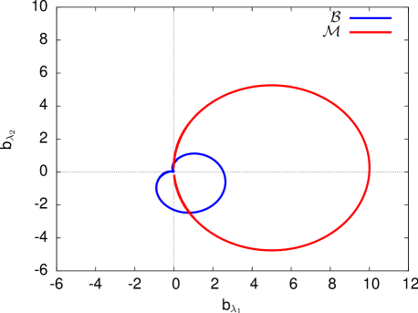
Figure 4: Hodograms calculated for a monopolar current distribution ($\mathcal{M}$) and bipolar one ($\mathcal{B}$).

The eigenvectors corresponding to the eigenvalues $\lambda_{1}$, $\lambda_{2}$ and $\lambda_{3}$, represent the direction of maximum, intermediate and minimum variance of the magnetic field respectively. The eigenvector corresponding to the minimum eigenvalue corresponds to the direction of minimum variance and is normal to the plane spanned by the magnetic field perturbations. This direction is observed to be parallel to that of the equilibrium magnetic field, shown in the same plot by a blue line. This confirms the hypothesis that the ELM filament is aligned with the equilibrium magnetic field. From the sense of the polarization the direction of the current is found to be colinear with the plasma current. The method allows the determination of the rotation matrix, so that the hodogram in the plane perpendicular to the current filaments may be reconstructed. This hodogram is shown in Figure 3 (b) together with a fit to an ellipse. The shape of the hodogram calculated in the rotated frame of reference can be used to determine the type of current distribution associated to an ELM. Theories have both proposed ELM filaments to be associated to monopolar Kirk et al. (2006a); Myra (2007) and bipolar current distributions Rozhansky and Kirk (2008). Up to now no clear evidence of one mechanism predominant with respect to the other has been reported. Figure 4 shows the anticipated shape of the hodogram in the bipolar and monopolar cases. The hodogram in the bipolar case exhibits a cardioid-like shape with a cusp at the origin, which represents a distinct signature and which can not be recognized in the experimental data (see Fig 3 (b)). To reinforce the statement we note that a bipolar-like hodogram with the presence of a cusp has been previously recognized in Spolaore et al. (2009) (cfr. fig 3(b)) where it has been associated to a direct measurement of a bipolar current structures. We emphasize, however, that the filaments observed in Spolaore et al. (2009) are of a completely different origin as induced by Drift-Alfvén turbulence Vianello et al. (2010). A further corroboration of the hypothesis of monopolar current filaments results from considering the quadrants occupied by the magnetic field trajectory. Indeed while the monopolar current hodogram regularly occupies two of the quadrants, the bipolar one always spans three of the quadrants: this latter behavior is not observed in the experimental data as can be verified by comparing Figure 3 (b) and Figure 4. These results make us confident that the magnetic fluctuations observed are indeed generated by a monopolar current distribution. Under this basic assumption the current carried by this filament may be estimated.

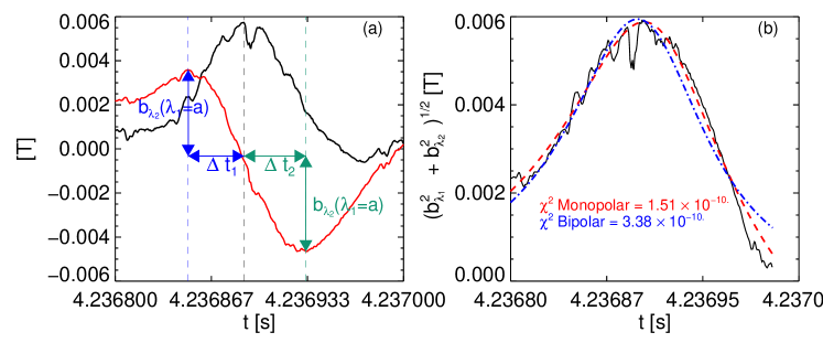
Figure 5: (a) Time traces of the two perpendicular components of magnetic field during an ELM filament. (b) Total perpendicular magnetic field as a function of time. Superimposed the results of a fit for an expected monopolar (red) and bipolar (blue) current distribution both modulated by an exponential decay.

In the rotated frame of reference for a circular monopolar symmetric filament drifting in the $\lambda_{1}$ direction, the two perpendicular magnetic field components may be written as $b_{\lambda_{1}}=\frac{-r_{0}B_{0}a}{\lambda_{1}^{2}+a^{2}}$ and $b_{\lambda_{2}}=-\frac{r_{0}B_{0}\lambda_{1}}{\lambda_{1}^{2}+a^{2}}$ where $B_{0}=\frac{\mu_{0}I_{0}}{2\pi r_{0}}$ and $a$ is the distance between the trajectory of the center of the filaments and the probe, representing also the distance of closest approach, $r_{0}$ is the radius of the filaments and $I_{0}$ its current. The distance $a$ can be approximated, assuming the filament to propagate with a constant velocity along the $\lambda_{1}$ direction: $a=\Delta tv_{\lambda_{1}}$ where $\Delta t$ is the time delay between the maximum of $b_{\lambda_{1}}$ and the maximum/minimum of $b_{\lambda_{2}}$, where $b_{\lambda_{1}}$ and $b_{\lambda_{2}}$ are the projections of the magnetic field in the maximum-intermediate variance plane. Thus within these approximations the current may be estimated noting that $|b_{\lambda_{2}}(\lambda_{1}=a)|=\frac{1}{2}\frac{\mu_{0}I_{0}}{2\pi a}=\frac{\mu_{0}I_{0}}{4\pi\Delta tv_{\lambda_{1}}}$ Applied to the experimental data, this computation is equivalent to calculate the quantities depicted in Figure 5, where $\Delta t$ has been calculated both at the maximum and at the minimum of $b_{\lambda_{2}}$. The two values $\Delta t_{1}$ and $\Delta t_{2}$ are equal to 38 $\mu$s and 42 $\mu$s respectively. The estimate of the current relies on the knowledge of local velocity in the $\lambda_{1}$ direction. This propagation has been reported for ASDEX Upgrade, e.g. Herrmann et al. (2008); Kirk et al. (2010). The experimental setup does not allow a reliable local measurements of $v_{r}$ or $v_{p}$, neither can we rely in the presented shots on correlation analysis of wall mounted probes (which are 160 degrees separated from the manipulator in the toroidal direction). Most likely these signals are indeed dominated by MHD mode activity in the confined plasma rather than current filaments in the SOL. As the best approximation we thus assume as radial propagation the most probable value $v_{r}=1.2$ km/s as determined in Kirk et al. (2010) and calculate $v_{\lambda_{1}}=v_{r}/\cos(\angle(\lambda_{1}-r))$, where $\angle(\lambda_{1}-r)$ is the nagle between $\lambda_{1}$ and the radial direction which for the present case is of the order of 7^∘. From Kirk et al. (2010) we also estimate a standard deviation of $v_{r}$ as $\sigma_{v_{r}}=700$ m/s, which ensure that 71 % of the events are observed within $(v_{r}\pm\sigma_{v_{r}})$. With these values the average distance of closest approach is approximately 4 cm and using the average value between the minimum and maximum of $b_{\lambda_{2}}$ we obtain an estimate of 1.9 kA.

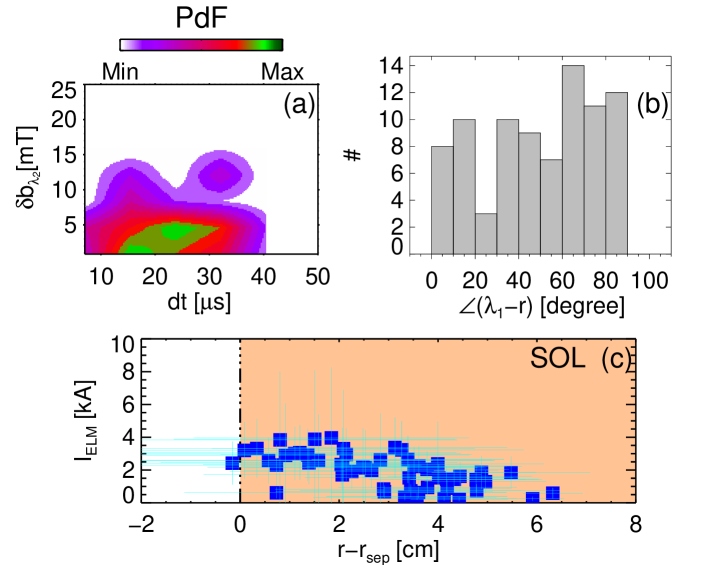
Figure 6: (a) Joint PDF of $\Delta t$ and $b_{\lambda_{2}}(\lambda_{1}=a)$ (b) )Histogram of the angle between $\lambda_{1}$ and the radial direction. (c) Filaments current estimate vs distance from the separatrix estimated with $v_{r}=1.2$ km/s. Error bars results from the propagation of velocity uncertainty in the estimate of $a$ and $I$.

The total perpendicular field $\sqrt{b_{\lambda_{1}}^{2}+b_{\lambda_{2}}^{2}}$ is shown in figure 5 (b). The magnetic field variation can be fitted with a function of the form $f=\left(\frac{\alpha}{\sqrt{(t-t_{0})^{2}+\beta}}-\gamma\right)e^{-(t-t_{0})/\tau_{e}}$, $t_{0}$ being the time instant corresponding to the maximum of the total perpendicular field and $\tau_{e}$ the e-folding time, and assuming the magnetic field is the response from a passing monopolar current filament. The good quality of the fit provides additional support for the monopolar nature of the filament, also comparing with the fit expected from a bipolar current distribution shown in blue line which exhibits an higher $\chi^{2}$. The average decay time is determined as $\tau_{e}\approx 200$ $\mu$s. In order to increase the statistic reliability of the previous estimate we have analyzed events from 5 different shots with similar conditions. The results are shown in Figure 6. In the panel (a) the joint PDF of the independent experimental values $\Delta t$ and $b_{\lambda_{2}}$ used for the current evaluation is shown, highlighting how the bulk of the filaments have values of approximately 25 $\mu s$ and 5 mT. In the panel (b) the histogram of the angle between $\lambda_{1}$ and the radial direction is shown, showing that the $\lambda_{1}$ direction is a complex combination of radial and poloidal propagation. Finally in the panel (c) the current estimated accordingly to the aforementioned formula is plotted vs the position of the filaments with respect to the separatrix, taking into account the position of the manipulator and the distance of closest approach estimated. The errors shown represent the influence of the velocity uncertainty on the estimate of $a$ and consequently on $I$. The bulk of the distribution of these filaments are thus observed in the SOL, even taking into account the uncertainty on $v_{r}$: the median of the distribution of the filaments detected in the SOL within the error in their position is 1.4 kA, corresponding to a $j_{\parallel}\approx 4.5MA/$m² for 1 cm radius filaments. These values are consistent with measurements of edge current as seen for example in Thomas et al. (2005). It has already been supposed in Wolfrum et al. (2008) that, in case ELM breakdown is driven by peeling instabilities, this will lead to a flattening of the current density profile over the separatrix and a subsequent increase of currents flowing into the SOL. These currents will be nearly force-free and will be accompanied by poloidal halo currents closing through the divertor tiles. Actually these currents have been measured Ionita et al. (2009); McCarthy et al. (2003) with values up to few tens of kA, supporting the presence of rapid flow of toroidal currents from the plasma into the SOL The resulting histogram may also be compared with the estimate for ELM filaments in JET given in P Migliucci and V Naulin (2010): in this case the most probable current has been found of the order of 450 A, but with a lower radial velocity postulated. For completeness it must be noted that the same current density was estimated in Herrmann et al. (2008) assuming the magnetic perturbation to be induced by a rotating helical structure with a bi-directional current close to, but still inside, the separatrix. The value found is higher than the measured $j_{sat}$ current density to the ion-biased tip (approximately 50 kA/m²). Concluding in this letter we have provided evidence that ELM filaments carry considerable currents for which we have found a reasonable estimate. The magnetic signals during ELM filaments differ substantially from wave activity in between ELMs. We have shown that the current in the filaments is co-aligned to the plasma current and approximately of a magnitude as expected for the edge. The current flows along the unperturbed magnetic field lines and has a unidirectional nature. This poses the question where the filament currents close in the SOL and why such high current densities are sustained in the ELM filaments. We hope that future experiments will contribute to answer these questions, which will throw new light on the instability mechanisms for ELMs.
This work, supported by the European Communities under the contract of Associations between EURATOM and ENEA, Risø/DTU, ÖAW Innsbruck, and IPP Garching, was carried out within the framework of the European Fusion Development Agreement. This work was also supported by project P19901 of the Austrian Science Fund (FWF).

References

- Fundamenski et al. (2007) W. Fundamenski et al., Plasma Phys. Control. Fusion 49, R43 (2007).
- Lui (2000) A. Lui, Ieee Trans. Plasma Sci. 28, 1854 (2000).
- Snyder et al. (2005) P. B. Snyder, H. R. Wilson, and X. Q. Xu, Phys. Plasmas 12, 056115 (2005).
- Kirk et al. (2006a) A. Kirk et al., Plasma Phys. Control. Fusion 48, B433 (2006a).
- Fenstermacher et al. (2005) M. Fenstermacher et al., Nucl. Fusion 45, 1493 (2005).
- Herrmann et al. (2007) A. Herrmann et al., J. Nucl. Mat. 363-365, 528 (2007).
- Kirk et al. (2006b) A. Kirk et al., Phys. Rev. Lett. 96, 185001 (2006b).
- Leonard et al. (2006) A. W. Leonard et al., Plasma Phys. Control. Fusion 48, A149 (2006).
- R Maqueda and R Maingi and NSTX team (2009) R Maqueda and R Maingi and NSTX team, Phys. Plasmas 16, 056117 (2009).
- Takahashi et al. (2008) H. Takahashi, E. D. Fredrickson, and M. J. Schaffer, Phys. Rev. Lett. 100, 205001 (2008).
- Herrmann et al. (2008) A. Herrmann et al., in in Proceedings of the 22nd Energy Fusion Conference, Geneva, IAEA-CN-165/ EX/P6-1 (2008).
- Ionita et al. (2009) C. Ionita et al., J. Plasma Fusion Res. Series 8, 413 (2009).
- Endler et al. (2005) M. Endler et al., Plasma Phys. Control. Fusion 47, 219 (2005).
- Samson and Olson (1980) J. Samson and J. Olson, Geophysical Journal International 61, 115 (1980).
- Santolík (2003) O. Santolík, Radio Sci. 38, 13 (2003).
- Weimer (2003) D. R. Weimer, J. Geophys. Res. 108, 12 (2003).
- Myra (2007) J. R. Myra, Phys. Plasmas 14, 102314 (2007).
- Rozhansky and Kirk (2008) V. Rozhansky and A. Kirk, Plasma Phys. Control. Fusion 50, 025008 (2008).
- Spolaore et al. (2009) M. Spolaore et al., Phys. Rev. Lett. 102, 165001 (2009).
- Vianello et al. (2010) N. Vianello et al., Nucl. Fusion 50, 042002 (2010).
- Kirk et al. (2010) A. Kirk et al., to be published on Plasma Phys. Contr. Fusion (2010).
- Thomas et al. (2005) D. Thomas et al., Phys. Plasmas 12, 056123 (2005).
- Wolfrum et al. (2008) E. Wolfrum et al., in Proceedings of the 22nd IAEA Energy Fusion Conference, Geneva (IAEA, 2008) pp. EX/P3–7.
- McCarthy et al. (2003) P. McCarthy et al., in In proceedings 30th EPS Conference on Plasma Physics, St.Petersburg, Vol. 27A (2003) pp. P–1.064.
- P Migliucci and V Naulin (2010) P Migliucci and V Naulin, Phys. Plasmas 17, 072507 (2010).