The Chemical Composition of Cernis 52 (BD+31^o 640)

Abstract

We present an abundance analysis of the star Cernis 52 in whose spectrum we recently reported the napthalene cation in absorption at 6707.4 Å. This star is on a line of sight to the Perseus molecular complex. The analysis of high-resolution spectra using a $\chi 2$-minimization procedure and a grid of synthetic spectra provides the stellar parameters and the abundances of O, Mg, Si, S, Ca, and Fe. The stellar parameters of this star are found to be $T_{\mathrm{eff}}=8350\pm 200$ K, $\log(g/{\rm cm~{}s}^{2})$$=4.2\pm 0.4$ dex. We derived a metallicity of $\mathrm{[Fe/H]}=-0.01\pm 0.15$. These stellar parameters are consistent with a star of $\sim 2$ M${}_{\odot}\;$in a pre-main-sequence evolutionary stage. The stellar spectrum is significantly veiled in the spectral range $\lambda\lambda 5150-6730$ Å up to almost 55 per cent of the total flux at 5150 Å and decreasing towards longer wavelengths. Using Johnson-Cousins and 2MASS photometric data, we determine a distance to Cernis 52 of 231${}^{+135}_{-85}$ pc considering the error bars of the stellar parameters. This determination places the star at a similar distance to the young cluster IC 348. This together with its radial velocity, $v_{r}=13.7\pm 1$ ${\rm km}\>{\rm s}^{-1}$, its proper motion and probable young age support Cernis 52 as a likely member of IC 348. We determine a rotational velocity of $v\sin i=65\pm 5$ ${\rm km}\>{\rm s}^{-1}\;$for this star. We confirm that the stellar resonance line of Li I at 6707.8 Å is unable to fit the broad feature at 6707.4 Å. This feature should have a interstellar origin and could possibly form in the dark cloud L1470 surrounding all the cluster IC 348 at about the same distance.

1 Introduction

In a recent study of the diffuse interstellar bands (DIBs) toward a region of anomalous microwave emission, Iglesias-Groth et al. (2008) have shown evidence for the presence of the naphthalene cation, ${\rm C}_{10}{\rm H}_{8}^{+}$, the simplest Policyclic Aromatic Hydrocarbon (PAH), in the line of sight towards the moderately reddened star Cernis 52 (BD+31^o 640, $V=11.4$, $E(B-V)=0.9$, Cernis 1993). The PAHs, including the naphthalene cation, have been also detected in a cometary dust sample returned to Earth by Stardust and in interplanetary dust particles, possibly of cometary origin (see the review by Li 2009).

Cernis 52 is an early type star, classified as A3V by Cernis (1993), has coordinates $\alpha=03^{\rm h}43^{\rm m}00.3^{\rm s}$ and $\delta=+31^{\circ}58^{\prime}26^{\prime\prime}$ (J2000.0), and is located at an angular separation of less than one degree from the very young stellar cluster IC 348 in the Perseus OB2 molecular complex. The photometric distance to star Cernis 52 is 240 pc (Cernis 1993), consistent with a location in the molecular complex OB2 where the microwave emitting cloud is also most likely located (see Watson et al. 2005). The uncertainties prevent to conclude whether the star is embedded in a cloud of this young star forming region or lay behind.

Iglesias-Groth et al. (2008) claimed that the relative strength of several diffuse interstellar bands detected in the spectrum of Cernis 52 was consistent with the presence of a molecular cloud in the line of sight. The anomalous microwave emission detected in the direction to Perseus (Watson et al. 2005, 2006) could be associated to electric dipole radiation of fast spinning hydrogenated carbon-based molecules in a molecular cloud, a mechanism originally proposed by Draine and Lazarian (1998). It is important to establish whether the cloud responsible for the excess color of Cernis 52 hosts the carriers of both, the diffuse interstellar bands observed in the spectrum of this star and the anomalous microwave emission detected in its line of sight.

Iglesias-Groth et al. (2008) also noted the near-coincidence in wavelength between the interstellar cation’s feature and the stellar Li I resonance line. To gain insight into the contribution of the stellar line to the observed broad feature, we undertook a thorough analysis by spectrum synthesis of Cernis 52’s spectrum with two principal goals - a general abundance analysis for the star and spectrum synthesis fits to the spectrum around 6707 Å in order assess the Li I line’s contribution.

Here we present a precise determination of the stellar parameters and a detailed chemical composition study of the star Cernis 52. This abundance analysis should provide indications of the likely Li abundance for the star, i.e., if the star is not chemically peculiar should have a lithium abundance no greater than the cosmic Li abundance of A(Li) $=3.3.$ In this paper we will discuss with special attention the naphthalene cation’s feature at 6707.4 Å in the spectrum of Cernis 52 and investigate the relationship of this star with the Perseus star forming region.

2 Observations

We have made use of spectroscopic data obtained with the 2dcoudé cross-dispersed echelle (CS23, Tull et al. 1995) at the 2.7 m Harlan J. Smith Telescope at McDonald Observatory (Texas, USA). We observed the star Cernis 52 on 26, 27 August 2007, and 1, 2 March 2008 in the spectral range $\lambda\lambda 3740-10160$ Å, with resolving power $\lambda/\delta\lambda\sim 60,000$ and $\sim 30,000$, respectively. These two datasets were independently reduced and properly combined to produce final spectra of SNR $\sim$150 and 250, respectively, at the position of H$\alpha$ for a dispersion of 0.05 Å/pixel.

We also performed spectroscopic observations with the cross-dispersed echelle spectrograph SARG (Gratton et al. 2001) at the Telescopio Nazionale Galileo (TNG) at the Observatorio del Roque de los Muchachos (La Palma, Canary Islands, Spain). We observed the target star on 4 November 2006 in the spectral ranges $\lambda\lambda 4600-7975$ and $\lambda\lambda 5600-10100$ Å, with a spectral resolution of $\lambda/\delta\lambda\sim 57,000$ and a final SNR $\sim 100$ at H$\alpha$ for a dispersion of 0.034 Å/pixel.

Early-type rapidly rotating hot stars were also observed for correction of possible telluric absorptions in all campaigns. All the spectra were reduced within IRAF, wavelength calibrated and co-added after correction for telluric lines.

3 Rotational and radial velocity

Firstly, each of the three final spectra was cross-correlated (within the package MOLLY) with a synthetic spectrum properly broadened with a $v\sin i=80$ ${\rm km}\>{\rm s}^{-1}$. Thus, we corrected these spectra for their radial velocities and derived a rotational velocity of $v\sin i=65\pm 5$ ${\rm km}\>{\rm s}^{-1}$by comparing broadened and veiled versions of a A3V synthetic spectrum in steps of 5 ${\rm km}\>{\rm s}^{-1}$, adopting an spherical rotational profile with linearized limb-darkening $\epsilon=0.46$, appropriate to the spectral type of the star (Al-Naimiy 1978).

Finally, we estimate a radial velocity of Cernis 52 at $v_{r}=+13.7\pm 1$ ${\rm km}\>{\rm s}^{-1}$. The cross-correlation was performed in the spectral range $\lambda\lambda 5140-6700$ Å and masking the broad H$\alpha$ profile and the interstellar features at 5889-95 Å and 6280 Å. This determination is consistent with the mean radial velocity of the young cluster IC 348, which has been recently estimated at $13.5\pm 1.2$ ${\rm km}\>{\rm s}^{-1}\;$from 30 near solar-mass cluster members (Dahm 2008). However, Nordhagen et al. (2006) derived a mean cluster velocity of $15.9\pm 0.8$ ${\rm km}\>{\rm s}^{-1}$, also from 30 cluster members.

We also determine a radial velocity of $14.2\pm 1.4$ ${\rm km}\>{\rm s}^{-1}\;$from the narrow atomic interstellar lines Na I D 5889-95 Å, Li I 6708 Å and K I 7698 Å. The uncertainty on the velocity comes from the dispersion of these velocity measurements.

These determinations share the velocity of the most luminous cluster member HD281159 ($\sim 14$ ${\rm km}\>{\rm s}^{-1}$, Evans 1967) and an expanding supernova shell in which the young cluster IC 348 is embedded ($\sim 12-15$ ${\rm km}\>{\rm s}^{-1}$, Snow et al. 1994). In addition, these atomic interstellar lines have a velocity consistent with that of the interstellar hyperfine transitions of the molecule ${\rm NH}_{3}$ measured in radio wavelegths (Rosolowsky et al. 2008): the LSR velocities are $7.5\pm 1.4$ ${\rm km}\>{\rm s}^{-1}\;$from the ISM lines and $6.1-8.4$ ${\rm km}\>{\rm s}^{-1}\;$from the radio transitions.

4 Companion star

Using the camera FastCam (Oscoz et al. 2008) attached to the Nordic Optical Telescope (NOT) at the Observatorio del Roque de los Muchachos, we obtained images in $V$, $R$ and $I$ bands of Cernis 52 on 25 October 2008. We found a companion star at a distance of $818\pm 7$ mas. This camera is able to obtain and record series of thousands of short exposures, and with a specially designed software can reach angular resolutions of roughly $0.1\arcsec$. In Fig. 1 we display the resulting image in the $R$ band. We have zoomed in the image to show the two stars clearly resolved. The camera has 512x512 pixels and a pixel size of $31.01\pm 0.01$ mas. The companion star is located in the North-West of Cernis 52, with a position angle North-East $\theta=325.9^{\circ}$.

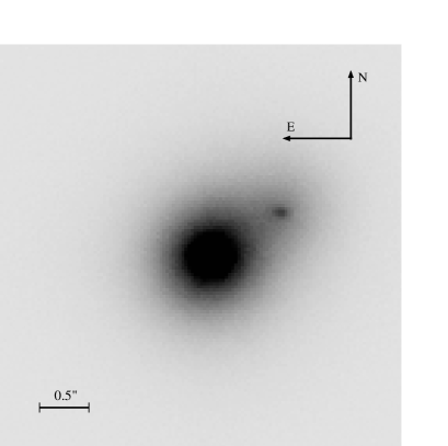
Figure 1: FastCam image in the $R$ band of Cernis [93]52. The displayed field size is $\sim 3.5\arcsec\times 3.5\arcsec$. There exists a companion star at a distance of $818\pm 7$ mas in the direction North-West of Cernis 52.

The companion star is roughly $1.7\pm 0.2$ mag fainter than Cernis 52 in the $R$ band. In our spectroscopic observations with the instrument CS23, obtained prior to the discovery of this companion star, the slit widths were $1.2\arcsec$ and $2.4\arcsec$ for the 2007 and 2008 campaigns, respectively. The slit length was $8.2\arcsec$ in both campaigns. Since the slit width was quite large and the seeing during the observations was typically $\simeq 2-2.5\arcsec$, most of the light from the companion star must have entered in the slit and contaminated the spectrum of Cernis 52. Assuming that the primary is A3V and that both stars are a physical pair we can estimate the spectral type of the companion from the observed magnitude difference in the R-band. We adopt a $T_{\rm eff}$ $=8500$ K and $\log\;g$ $=4.0$ for the primary. Thus, we find a probable $T_{\rm eff}$ $=5800$ K for the companion from suitable bolometric corrections (Bessell et al. 1998) and assuming that both stars share the same color excess. Thus, we search for evidence of the spectrum of a solar-type companion in the 2007 and 2008 final spectra of Cernis 52. We cross-correlated these spectra with the spectrum of the Sun (Kurucz et al. 1984), properly broadened with different rotational velocities and in a radial velocity range from -150 to 150 ${\rm km}\>{\rm s}^{-1}$, but we did not find any clear signature of this star in the cross-correlation function.

It is likely that the companion star have slightly contaminated the spectrum of Cernis 52. From the magnitude difference in the $R$ band and taking into account that the companion star was partially out from the slit, we estimate the flux ratio of both stars in our spectrum at $F_{\rm sec}/F_{\rm C52}=0.11\pm 0.05$ in the wavelength region corresponding to the $R$ band. However, as we will see this is not sufficient to explain the level of veiling found in the analysis of the photospheric features of Cernis 52. There must be another reason for the apparent weakness of the stellar features.

In Fig. 2 we display an optical image from the Palomar Digital Sky Survey of Cernis 52 with a field size of $5\arcmin\times 5\arcmin$. In this DSS-2 red image one can see an entended emission of interstellar gas surrounding the star which may be the reason why the spectrum of Cernis 52 is veiled. Our spectra were not background subtracted, since the star is very bright and the raw images do not show any clear sky line. However, in the raw images there is neither any indication of the presence of this nebulosity, appart from the high number of counts of the sky, and any signal must have been subtracted when correcting for the scattered light. In Fig. 2 we see that the interstellar cloud is more prominent towards the North of the star, $\sim 0.5\arcmin$ from the star center. However, we do not see any asymmetry in the signal of the sky spectrum which may indicate that the slit was not positioned South$-$North. The interstellar cloud may have contaminated our spectra but we suspect that most of the light coming from the cloud must have been subtracted during the data reduction. A discussion of the interstellar emission in the proximity of Cernis 52, using Spitzer data, is deferred to a forthcoming paper (S. Iglesias-Groth et al. 2009, in preparation).

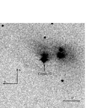
Figure 2: DDS-2 image in the $R$ band of Cernis [93]52. The displayed field size is $\sim 5\arcmin\times 5\arcmin$.

In the next section, we will concentrate on the determination of the stellar parameters of Cernis 52, taking into account any possible source of veiling in the spectrum, whose flux we will denote as $F_{\rm veil}$.

5 Stellar Parameters

Table 1: Ranges and steps of model parameters

Parameter	Range	Step
$T_{\mathrm{eff}}$ (K)	$7850\rightarrow 8750$	100
$\log(g/{\rm cm~{}s}^{2})$	$3.\rightarrow 5$	0.1
$\mathrm{[Fe/H]}$	$-0.5\rightarrow 0.5$	0.05
$f_{6562}$	$0\rightarrow 1.0$	0.05
$m_{0}$ (Å-1)	$0\rightarrow-0.001$	-0.0001

We have inspected the spectrum of Cernis 52 to search for atomic stellar lines appropriate to provide accurate element abundances. We realized that the stellar lines were significantly veiled even at a level of $\sim 50$ per cent at 5180 Å where the Mg Ib triplet is located. Thus, the Fe abundances obtained from the lines Fe I 5214 Å and Fe II 5273 Å if we do not include any veiling are [Fe/H] $=-0.55$ and -0.8, respectively. This metallicity seems to be too low for the location of this star in a star-forming region. In addition, the Mg Ib 5172 Å would require an abundance of [Mg/Fe]$\sim-1.0$. These results are achieved for all reasonable values of the atmospheric parameters, $T_{\rm eff}\;$and $\log\;g$. The analysis of this spectrum requires a tool able to take into account the effect of any possible veiling when computing atmospheric abundances. To simplify, we assumed the veiling to be a linear function of wavelength, and thus defined by two parameters, its value at 6562 Å, $f_{6562}=F^{6562}_{\rm veil}/F^{6562}_{\rm C52}$, and the slope, $m_{0}$. Note that the total flux is defined as $F_{\rm total}=F_{\rm veil}+F_{\rm C52}$, where $F_{\rm veil}$ and $F_{\rm C52}$ are the flux contributions of the source of veiling and the continuum of Cernis 52, respectively. We decided to split the determination of the stellar and veiling parameters in two steps: 1) using the H$\alpha$ profile to derive the stellar temperature and the veiling at 6562 Å; and 2) using Fe I and Fe II features to derive the surface gravity, the slope of the veiling and the metallicity of Cernis 52.

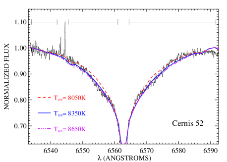
Figure 3: Synthetic H$\alpha$ profiles for three effective temperatures compared to the observed spectrum of Cernis 52 (SNR $\sim 150$) and normalized to the level of the observed spectrum of Cernis 52 at 6540 Å. We also depict the fitting regions at the top.

5.1 H$\alpha$ Profile

The wings of H$\alpha$ are a very good temperature indicator (e.g., Barklem et al. 2002). Adopting the theory of Ali & Griem (1965, 1966) for resonance broadening and Griem (1960) for Stark broadening, we computed H$\alpha$ profiles for several effective temperatures, using the code SYNTHE (Kurucz 2005; Sbordone 2005). For further details on the computations of hydrogen lines in SYNTHE, see Castelli & Kurucz (2001) and Cowley & Castelli (2002).

In this section, we will use the spectrum of Cernis 52 taken in 2007 since the 2008 spectrum had a different wavelength setting and the H$\alpha$ line appears in an interorder region. In Fig. 3 we compare the synthetic H$\alpha$ profiles with the observed profile for several temperatures. To evaluate the goodness of fit, we employ a reduced $\chi 2$ statistic,

$$\chi_{\nu}^{2}=\frac{1}{N-M}\sum^{N}_{i=1}\left(\frac{f_{i}-F_{i}}{\sigma_{i}}\right)2,$$ (1)

where $N$ is the number of wavelength points, $M$ is the number of free parameters (here two, $T_{\rm eff}\;$and $f_{6562}$), $f_{i}$ is the synthetic normalized flux, $F_{i}$ is the observed normalized flux, and $\sigma_{i}=1/{\rm SNR}$. The SNR was estimated as a constant average value in continuum regions close to the observed H$\alpha$ profile. The fitting regions are indicated in Fig. 3, which contains all of the spectral regions close the center of the H$\alpha$ profile where there are no stellar lines and where the normalized flux is greater than $\sim 0.7$. This figure also shows that the sensitivity of this method to the $T_{\rm eff}\;$decreases toward higher effective temperatures.

In order to estimate the uncertainties on temperature and veiling, we built 1000 realizations of the observed spectrum taking into account the SNR. We used a boostrap Monte Carlo method to define the 1-$\sigma$ confidence regions and found as most likely values $T_{\mathrm{eff}}=8300\pm 100$ K and $f_{6562}=0.50\pm 0.05$. The corresponding histograms are displayed in Fig. 4. The $T_{\rm eff}\;$and $f_{6562}$ were varied within the ranges given in Table 1. To check the influence of the spectrum of the companion star we perform another simulation by introducing the H$\alpha$ profile of a pre-main sequence solar metallicity star with $T_{\rm eff}\;$$=5800$ K and $\log\;g\;$$=3.8$, and assuming that this spectrum was contributing with the 10% of the stellar flux. The adopted surface gravity for the companion star coincides with the expected value for a pre-main sequence star of this temperature (see Section 6). We use a rotational velocity of $v\sin i=100$ ${\rm km}\>{\rm s}^{-1}\;$and a limb-darkening coefficient $\epsilon=0.6$, because the spectrum of Cernis 52 does not show any stellar narrow absorption and also to be consistent with the synthetic spectra computed for Section 6. However, we check that using lower rotational velocities does not affect the derived $T_{\rm eff}$. The result is shown in Fig. 5. The distribution of temperatures slightly changes but our adopted effective temperature remains almost the same, $T_{\mathrm{eff}}=8350\pm 100$ K. In contrast, the required veiling factor changes, being in this case $f_{6562}=0.40\pm 0.05$.

5.2 Ionization Equilibrium of Iron

Once we have determinated the veiling at 6562 Å and the effective temperature we try to derive the surface gravity and metallicity using Fe I and Fe II features of the spectrum of Cernis 52. In this case, we will neglect the presence of a companion spectrum since it hardly affects the spectrum of Cernis 52. We use a technique which compares a grid of synthetic spectra with the observed spectrum, via a $\chi 2$-minimization procedure. In this case, we will use the spectrum of Cernis 52 taken in 2008, since it has higher SNR. This procedure takes into account the effect that veiling causes on the stellar lines and it has been applied in X-ray binaries to derive the stellar parameters of the companion stars in these systems (A0620–00, González Hernández et al. 2004; Centaurus X-4, González Hernández et al. 2005; XTE J1118+480, González Hernández et al. 2006, 2008b; and Nova Scorpii 1994, González Hernández et al. 2008a). However, we needed to slightly modify this program in order to allow a fixed veiling at a given wavelength. In the previous version of this program, the slope of the veiling was defined using a given veiling at 4500 Å. We typically produce 10 different values for the slope, whose maximum value is zero, i.e. a constant veiling, and the minimum value provides a veiling of $f_{6562}=0.50$ and $f_{5000}=2$ (see Table 1).

Figure 4: Normalized distributions obtained for the effective temperature, $T_{\rm eff}$, measured from the H$\alpha$ profile and the veiling at 6562 Å, $f_{\rm 6562}$, using Monte Carlo simulations. The total number of simulations was 1000.

Figure 5: Same as Fig. 4, but including the spectrum of the Sun with a contribution of 10% of the stellar flux.

We already know the veiling at 6562 Å, but we need also to find the slope of the veiling in order to properly model the observed features. We selected 10 spectral features of iron in the spectral range $\lambda\lambda 5270-6400$ Å, containing in total 55 lines of Fe I and 25 lines of Fe II with excitation potentials between 0.5 and 10.5 eV. We compute synthetic spectra with the local thermodynamic equilibrium (LTE) code MOOG (Sneden 1973), adopting the atomic line data from the Vienna Atomic Line Database (VALD, Piskunov et al. 1995) and using a grid of LTE model atmospheres (Kurucz 1993). The oscillator strengths of the iron lines as well as other element lines used in this work were adjusted until reproducing both the solar atlas of Kurucz et al. (1984) with solar abundances (Grevesse et al. 1996) and the spectrum of Procyon with its derived abundances (Andrievsky et al. 1995). We generated a grid of synthetic spectra for the Fe I and Fe II features varying as free parameters, the star effective temperature ($T_{\mathrm{eff}}$), the surface gravity ($\log g$), the metallicity ([Fe/H]), and the veiling, charaterized by the $f_{6562}$ and $m_{0}$. The microturbulence, $\xi=2$ ${\rm km}\>{\rm s}^{-1}$, was fixed in each atmospheric model according to the spectral type of Cernis 52 (see e.g. Fossati et al. 2008). We choose an error of 0.5 ${\rm km}\>{\rm s}^{-1}\;$for the microturbulent velocity.

Figure 6: Normalized distributions obtained for the effective temperature, $T_{\rm eff}$, surface gravity, $\log\;g$, metallicity, [Fe/H], and veiling slope, $m_{0}$, using Monte Carlo simulations. The labels at the top of each bin indicate the number of simulations consistent with the bin value. The total number of simulations was 1000.

We fixed the veiling parameter at $f_{6562}=0.50$ and allowed the effective temperature to be in the range $8250<$ $T_{\rm eff}$ $<8450$. The other three free parameters were varied using the ranges and steps given in Table 1. We use a bootstrap Monte-Carlo method to derive the resulting histograms of these parameters shown in Fig. 6, corresponding again to 1000 realizations. We found strong evidence of high veiling in the spectral region under analysis (5270–6400 Å). This veiling increases toward shorter wavelengths, being as high as $f_{5180}\sim 1.2$ at the Mg Ib triplet 5167–83Å. This translates into a veiling of roughly 54% when computing the ratio of the flux $F^{5180}_{\rm veil}$ to the total flux, $F^{5180}_{\rm total}$. Therefore, at 5180 Å the star contributes almost with half of the total flux. By inspecting the histograms displayed in Fig. 6, we decided to choose as most likely values: $T_{\mathrm{eff}}=8350\pm 200$ K, $\log(g/{\rm cm~{}s}^{2})=4.2\pm 0.4$, $\mathrm{[Fe/H]}=0.20\pm 0.15$, $f_{6562}=0.50\pm 0.10$, and $m_{0}=-0.00055\pm 0.00010$. These stellar parameters are consistent with the spectral type already reported by Cernis (1993).

The surface gravity is the stellar parameter that is usually more difficult to determine when dealing with fast rotating and veiled stars (see e.g. González Hernández et al. 2005, 2008b). We warn the reader that the error bar given for the surface gravity comes from the range of values that shows the histogram of this parameter in Fig 6.

Table 2: Chemical Abundances of Cernis 52

Species	$\log\epsilon(\mathrm{X})_{\odot}$	$[{\rm X}/{\rm H}]$	$[{\rm X}/{\rm Fe}]$	${\sigma}$	$\Delta_{\sigma}$	$\Delta_{T_{\rm eff}}$	$\Delta_{\log g}$	$\Delta_{\rm veil}$	$\Delta_{\xi}$	$\Delta\mathrm{[X/H]}$	$N$
O I	8.74	0.54	0.55	0.28	0.20	0.00	0.03	0.15	-0.10	0.27	2
Mg I	7.58	0.35	0.36	0.25	0.25	0.20	-0.05	0.15	-0.30	0.47	5173
Si II	7.55	-0.10	-0.09	0.28	0.20	0.00	0.03	0.10	-0.15	0.27	2
S I	7.33	-0.19	-0.18	0.04	0.02	0.10	0.00	0.05	0.00	0.11	2
Ca I	6.36	-0.02	-0.01	0.22	0.08	0.17	-0.02	0.07	-0.05	0.21	7
Ca II	6.36	0.10	0.11	0.25	0.25	0.10	0.10	0.05	0.00	0.29	5307
Fe I	7.50	0.03	0.04	0.19	0.05	0.13	0.01	0.05	-0.03	0.15	13
Fe II	7.50	-0.06	-0.05	0.08	0.03	0.07	0.04	0.04	-0.06	0.11	8

Note. — Chemical abundances of Cernis 52 and uncertainties produced for $\Delta_{T_{\rm eff}}=+200$ K, $\Delta_{\log g}=+0.4$ dex, $\Delta_{\rm veil}=+0.1$, and $\Delta_{\xi}=+0.5~{}$${\rm km}\>{\rm s}^{-1}$. All the element abundances were determined by fitting the observed spectra with synthetic spectra computed with the LTE code MOOG.

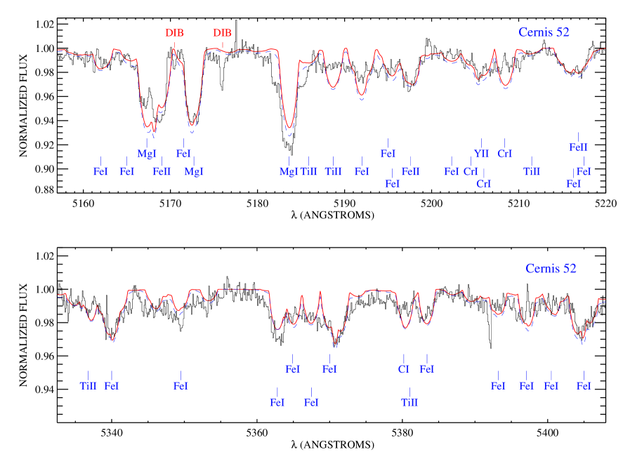
Figure 7: Best synthetic spectral fits (solid lines) to the observed spectrum of Cernis 52 for two spectral regions. We also display the combined spectrum (dashed line) including the spectrum of Cernis 52 contributing with 92% (top panel) and 91% (bottom panel) of the stellar flux and the spectrum of the companion star contributing at 8 and 9%, respectively. Note that the veiling factors $f_{5180}=1.25$ and $f_{5370}=1.15$ have been adopted. The label “DIB” refers to diffuse interstellar bands, whereas other labels show stellar absorption lines of Cernis 52.

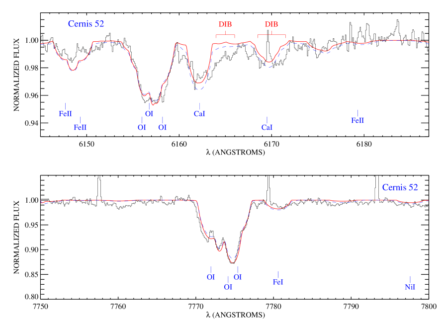
Figure 8: Same as Fig. 7, but for other spectral regions. In this case, the best fit abundance of each feature has been used, being [O/H] $=0.74$ in the upper panel and [O/H] $=0.34$ in the lower panel. We also display the combined spectrum (dashed line) including the spectrum of Cernis 52 contributing with 90% (top panel) and 87% (bottom panel) of the stellar flux and the spectrum of the companion star contributing at 10 and 13%, respectively. Note that the veiling factors $f_{6157}=0.75$ and $f_{7773}=0$ have been adopted.

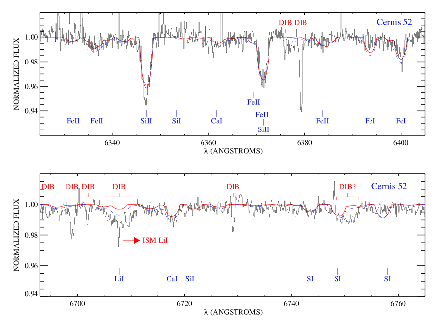
Figure 9: Same as Fig. 7, but for other spectral regions. We also display the combined spectrum (dashed line) including the spectrum of Cernis 52 contributing with 90% (both panels) of the stellar flux and the spectrum of the companion star contributing at 10%, respectively. In the bottom panel, the solid line show a synthetic spectrum of Cernis 52 with A(Li) $=3.3$, whereas the dashed line shows a combined spectrum in which both Cernis 52 and the companion star have A(Li) $=3.3$. Note that the veiling factors $f_{6360}=0.60$ and $f_{6720}=0.40$ have been adopted. The label “ISM LiI” gives the location of the atomic Li interstellar line.

6 Photospheric abundances

Using the derived stellar and veiling parameters, we firstly determined the abundance of Fe from each individual feature of Fe I and Fe II in the observed spectrum (see Table 2). We made use of a $\chi 2$ procedure to find the best fit to the observed features as in González Hernández et al. (2004, 2008a). In Fig. 7 we show some of the spectral regions analysed to obtain the Fe abundance. To determine the abundances of other elements, we adopted the average abundance of the Fe abundances extracted from Fe I and Fe II features, ${\rm[Fe/H]}=-0.01\pm 0.15$, for the metallicity of the model.

In Table 2 we provide the average abundance of each element together with the errors. The errors in the element abundances show their sensitivity to the uncertainties in the effective temperature ($\Delta_{T_{\mathrm{eff}}}$), surface gravity ($\Delta_{\log g}$), microturbulence ($\Delta_{\xi}$), veiling ($\Delta_{\rm veil}$) and the dispersion of the abundance measurements from different spectral features ($\Delta_{\sigma}$). The errors $\Delta_{\sigma}$ were estimated as $\Delta_{\sigma}=\sigma/\sqrt{N}$, where $\sigma$ is the standard deviation of the $N$ measurements. For those element species for which only one spectral feature was available we adopt $\sigma=0.25$. The total error in the abundance of each element is determined by adding in quadrature all these individual errors.

In Figs. 7, 8 and 9 we display several spectral regions of the observed spectrum of Cernis 52 in comparison with synthetic spectra computed using the derived abundances, except for oxygen, for which the best fit abundance was used for each feature. In these figures, we also show the combined synthetic spectrum of Cernis 52 and the companion star in which the companion star only contributes with $\sim 10$% of the stellar flux, and using the same veiling factors as for the single synthetic spectrum of Cernis 52. The stellar parameters, metallicity and radial velocity of the companion star were already specified in Section 5.1. We assumed that the radial velocity of the companion star is the same as for Cernis 52. For most of the features, the presence of the companion do not change significantly the line profiles, except for the Mg Ib 5167–83Å lines and the Ca I features. We note that we have not taken into account the presence of the companion star in the abundance determination, since this effect would be negligible and in any case, the abundances would remain within the error bars given in Table 2.

Table 3: Distance to Cernis 52

Parameter	$E(B-V)\tablenotemark{a}=0.9$	$T_{\rm eff}\;$$\tablenotemark{b}=8550$ K	$\log\;g\;$$\tablenotemark{b}=3.8$	$\log\;g\;$$\tablenotemark{b}=4.6$	$E(B-V)\tablenotemark{b}=0.8$	$M_{\star}\tablenotemark{b}=2.2~{}\hbox{\hbox{M}${}_{\odot}$}$
$d_{m_{V}}\tablenotemark{c}$ (pc)	$237\pm 9$	$247\pm 9$	$378\pm 14$	$149\pm 9$	$273\pm 5$	$249\pm 10$
$d_{m_{R}}$ (pc)	$229\pm 10$	$237\pm 10$	$363\pm 16$	$144\pm 11$	$256\pm 6$	$240\pm 11$
$d_{m_{I}}$ (pc)	$247\pm 10$	$253\pm 11$	$390\pm 17$	$157\pm 11$	$268\pm 6$	$259\pm 11$
$d_{m_{J}}$ (pc)	$233\pm 2$	$237\pm 2$	$369\pm 3$	$147\pm 2$	$242\pm 1$	$245\pm 2$
$d_{m_{H}}$ (pc)	$232\pm 2$	$235\pm 2$	$367\pm 4$	$147\pm 3$	$238\pm 1$	$243\pm 2$
$d_{m_{K}}$ (pc)	$227\pm 1$	$230\pm 1$	$359\pm 2$	$144\pm 2$	$231\pm 1$	$238\pm 1$
$d_{\rm av}^{d}$ (pc)	$231\pm 8$	$238\pm 8$	$366\pm 12$	$146\pm 5$	$257\pm 18$	$252\pm 9$

7 Discussion

7.1 Membership in IC 348

As shown in Section 3, the radial velocity of Cernis 52 is consistent with the mean radial velocity of known members of the cluster IC 348.

The membership of a star in a cluster is generally established if the star is located nearby on the plane of the sky and its radial velocity and proper motion coincide with those of the cluster. Fortunately, the proper motion of Cernis 52 has been measured with high accuracy by Röser et al. (2008), providing $(\mu_{\alpha}\cos\delta$, $\mu_{\delta}=(+7.22$,$-8.62)\pm(1.5$,$1.6)$ mas yr^-1.

The proper motion of the cluster IC 348 has been determined by Scholz et al. (1999) in several systems. In particular, using the Hipparcos system, they derive a mean proper motion of ($\mu_{\alpha}\cos\delta$, $\mu_{\delta}=(+4.6$,$-8.3)\pm(3.7$,$1.6)$ mas yr^-1, from nine Hipparcos stars of the cluster IC 348.

More recently, the measurement of proper motion of this cluster has been improved considerably by Loktin & Beshenov (2003). They determine a proper motion of $(\mu_{\alpha}\cos\delta$, $\mu_{\delta}=(+6.87$,$-9.15)\pm(0.56$,$0.49)$ mas yr^-1.

The radial velocity and proper motion of Cernis 52 strongly support its membership in the young cluster IC 348. In addition, the nine stars studied by Scholz et al. (1999) provide a mean distance of $261^{+27}_{-23}$ pc. Therefore, Cernis 52 must be located at this distance. In the following subsections we will discuss the mass, radius, age, luminosity and distance of Cernis 52.

7.2 Mass, Radius and Age

In Fig. 10 we depict theoretical evolutionary tracks for pre-main sequence stars from Siess et al. (2000). We also overplot the position of Cernis 52 which seems to be consistent with a theoretical $2.0\pm 0.2$ M${}_{\odot}\;$star with an age of $3-20$ Myr. The position of the star is in between the theoretical tracks with masses 2.2 and 1.8 M${}_{\odot}\;$. These masses and the derived $\log\;g\;$imply a radius in the range $1.1<R/R_{\odot}<2.8$.

The young cluster IC 348 has an age of 3–7 Myr, according to Trullols & Jordi (1997), from a sample of 123 stars in a wide range of spectral types. Their analysis relies on photometric data and is possibly affected by unknown extinctions. Luhman et al. (2003) discuss the age of IC 348 in detail and claimed that the observational data seems to imply ages ranging from 1 to 10 Myr, although it favours a mean age of 2 Myr. They used photometric data of a large sample of K7-M8 spectral-type stars, although they also obtained spectroscopic data. Herbig (1998) also studied the age of roughly 100 stars of this cluster and found a spread between 0.7 and 12 Myr. All these studies depend on spectral-type classifications which may be uncertain, however, they seem to support that the age of IC 348 likely range between 1 and 12 Myr. The position of Cernis 52 in Fig. 10 is in agreement with the most likely age range for the cluster IC 348.

7.3 Luminosity and Distance

There is no available paralax for Cernis 52. Here, we estimate the distance to Cernis 52 from different photometric magnitudes taking into account the stellar parameters. We know the photometric magnitudes in five different filters: $m_{V}=11.4\pm 0.1$ (from Cernis 1993), $m_{R}=10.65\pm 0.10$ and $m_{I}=10.04\pm 0.10$ mag, and $m_{J}=8.91\pm 0.02$, $m_{H}=8.49\pm 0.03$, and $m_{K_{\rm s}}=8.27\pm 0.02$ mag from the 2MASS catalog. Except for the 2MASS magnitudes, we adopted ad hoc the values for the uncertainties on the photometric magnitudes of Cernis 52. We derived the radius of the star from the surface gravity, $\log(g/{\rm cm~{}s}^{2})$ $=4.2\pm 0.4$ dex, and assuming a mass of 2  M_⊙. This radius, together with the spectroscopic estimate of the effective temperature, $T_{\rm eff}\;$$=8350\pm 200$ K, provides an intrinsic bolometric luminosity in the range $5.4<L_{\star}/L_{\odot}<34.2$. We determined the absolute bolometric magnitude from the following formula: $M_{\rm bol,\star}-M_{\rm bol,\odot}=-2.5\log(L_{\star}/L_{\odot})$, where the solar bolometric magnitude is $M_{bol,\odot}=4.75$ (IAU simposium 1999) and the solar luminosity is $L_{\odot}=3.847\,\times\,10^{33}$ erg s^-1.

The apparent bolometric magnitude, $m_{\rm bol,\star}=m_{i,0}-BC_{i}$, was derived using the bolometric corrections, $BC_{i}$, for non-overshooting ATLAS 9 models (Bessell, Castelli, & Plez 1998). The bolometric corrections were determined as $BC_{i}=BC_{V}+V-i$. For the 2MASS infrared magnitudes we computed the theoretical colors $V-i$, for $i=J$, $H$, $K_{\rm s}$, from González Hernández & Bonifacio (2009).

We adopt the color excess, $E(B-V)=0.9$ mag, from Cernis (1993) which seems to provide consistent distances when using optical and infrared magnitudes. We compute the magnitude corrected for extinction in each filter as $m_{i,0}=m_{i}-A_{i}$, where $A_{i}$ were obtained using the relation $A_{i}=R_{i}E(B-V)$, with $R_{i}$, the ratio of total to selective extinction, given by the coefficients provided in McCall (2004). This author gives $R_{V}=3.07$ with deviations unlikely to exceed 0.05. Note that using a different value, e.g. $R_{V}=3.31$ as derived for Cernis 77 (BD+31^o 643) in Snow et al. (1994) or $R_{V}=3.2$ as in Cernis (1993), lead to small corrections to the distance determination, by –21 and –12 pc respectively.

The apparent magnitude, $m_{i}$, was decontaminated from the magnitude of the companion star, according to the stellar parameters derived in Section 4. We estimate the flux ratio of both stars, $F_{\rm sec}/F_{\rm C52}$, from theoretical magnitudes which were interpolated in the grid of theoretical colors $V-R$ and $V-I$ (Bessel et al. 1998) and the color $V-K$ and magnitudes $J$, $H$, $K_{\rm s}$ (González Hernández & Bonifacio 2009). Finally, the corrected magnitude is derived from the following expression

$$m_{i}=m_{21,i}+\log(F_{21,i}+1)$$

where $m_{i}$ is the corrected magnitude in the filter $i$, $m_{21,i}$ is the observed magnitud which contains the flux of both stars, and $F_{21,i}$, the flux ratio $F_{\rm sec}/F_{\rm C52}$ in the filter $i$. In Table 3 we show the derived distance for each filter with different sets of the relevant parameters. Note that the relatively small formal error in the distance estimate for each filter is calculated by assuming the magnitudes equal $m_{i}+\Delta m_{i}$.

Figure 10: Theoretical evolutionary tracks from Siess et al. (2000) for pre-main sequence stars with masses 1.8, 2.0 and 2.2 M${}_{\odot}\;$and for solar metallicity, $Z=0.02$. The different ages of the tracks refer to the age of a star at the end of the track, i.e. close the main sequence. The filled circle represents the position of Cernis 52. The triangles and squares following the tracks represent the position of the theoretical stars at the age of 3 and 9 Myr respectively.

We have derived a distance of 231${}^{+135}_{-85}$ pc for the star Cernis 52, according to the adopted stellar parameters and mass in section 5.2 and 7.2. Cernis (1993) argued that the star Cernis 52 is a member of the young cluster IC 348. This author derived a distance to Cernis 52 of 236 pc from the $V$ magnitude, adopting a spectral type of A3V and a color excess $E(B-V)=0.9$. He also derived a distance to the cluster IC 348 of $260\pm 16$ pc from 13 probable members of the cluster. Trullols & Jordi (1997) provide a photometric determination of the distance to IC 348 based on the filter $V$ of $240^{+128}_{-84}$ pc from 43 cluster members. These distance determinations rely on spectral type classification. Herbig (1998) argued that spectral types derived from spectroscopy would produce types somewhat later, and thus smaller $A_{V}$, and concluded that the Trullols & Jordi (1997) photometric distance should correspond to a spectroscopic distance of 276 pc. Our distance determination to Cernis 52 seems to be in agreement with that of the young cluster IC 348.

To sum up, all the arguments provided in this paper support Cernis 52 as being a member of the young cluster IC 348, and place the star far enough to explain the large color excess, and the presence of the interstellar features recently discovered by Iglesias-Groth et al. (2008). These intestellar features must be caused by the known dark clouds already mentioned by Cernis (1993), in particular, the dark cloud L1470 which covers all the young cluster IC 348.

7.4 Photospheric abundances

The O I triplet 6156–8 Å required a high O abundance ([O/H] $=0.5$), whereas the best fit abundance of the O I triplet 7771–5 Å is [O/H] $=0.15$ (see Fig. 8). This is unexpected since the O I triplet at 7771–5 Å shows stronger negative NLTE corrections than the O I triplet 6156–8 Å (Baschek et al. 1977). This may indicate the existence of some veiling at 7773 Å, instead of the zero value adopted (according to the extrapolation of the veiling previously derived as a function of wavelength). Similar problems are found in the Mg Ib triplet 5167–83 Å (see Fig. 7). For these features we depict the synthetic spectra computed using the best fit abundance given by the feature Mg I 5173 Å, and this abundance is unable to reproduce both Mg features at 5167 and 5183 Å. There are other features over the whole spectrum that cannot be reproduced with the synthetic stellar spectra which may be related to the presence of unknown DIBs. We emphasize that for the chemical abundance analysis we have chosen only those features that are not affected by any known interstellar absorption band.

The photospheric abundances of the star seems to be almost solar within the error bars, i.e., the star does not belong to the group of chemically peculiar (CP) A-type stars. There appears to be a correlation between the presence of chemical anomalies and the rotational velocity of these stars (e.g. Fossati et al. 2008; Takeda et al. 2008). Thus, stars with $v\sin i\lesssim 50-75$ ${\rm km}\>{\rm s}^{-1}\;$are underabundant in O and Ca (down to [X/H]$\sim-0.8$), and overabundant in Fe ([Fe/H]$\sim 0.5$) and specially Ba (up to [Ba/H]$\sim 1.5$), whereas Si and S shows near-solar abundances. Cernis 52 has a rotational velocity on the edge between “peculiar” and “normal” A stars. In the bottom panel of Fig. 11, we depict the Ba line which gives an abundance [Ba/H]$\sim-0.8$, which is even lower than the solar abundance. This definitively discards Cernis 52 as a chemically peculiar A-type star.

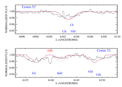
Figure 11: Same as Fig. 7, but for other spectral regions. Upper panel: synthetic spectra are computed with A(Li) $=4.0$ (solid line) and A(Li) $=3.3$ (dashed line). We emphasize that A(Li) $=3.3$ must be the maximum Li abundance in this star (see Section 7.5). Bottom panel: synthetic spectra are computed with [Ba/H] $=-0.8$ (solid line) and [Ba/H] $=-0.1$ (dashed line).

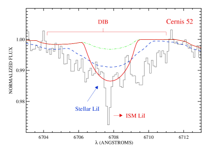
Figure 12: Same as Fig. 7, but for other spectral region. Synthetic spectra are computed with A(Li) $=4.0$ (solid line) and A(Li) $=3.3$ (dashed-dotted line). We also display the combined spectrum (dashed line) including the spectrum of Cernis 52 contributing with 90% of the stellar flux and the spectrum of the companion star contributing at 10%, respectively. The dashed line shows a synthetic spectrum with A(Li) $=3.3$ and 4.0, for Cernis 52 and the companion, respectively.

7.5 The naphthalene feature at 6707.4 Å

In our paper announcing the discovery of the naphthalene cation (Iglesias-Groth et al. 2008), we noted that the strongest band of the interstellar cation appeared at 6707.4 Å, i.e. very close to the stellar Li I resonance line. The abundance analysis presented in this paper was expected to provide indications of the likely Li abundance for the star, i.e., a star without abundance anomalies is very likely to have a lithium abundance no greater than the local abundance of A(Li)$=3.3$ (see bottom panel of Fig. 9).

In Fig. 12 we show three synthetic spectra: (i) two of them computed only considering the star Cernis 52 and with a already too high Li abundance, A(Li) $=4.0$ and a cosmic Li abundance, A(Li) $=3.3$, and, (ii) the other combining the spectrum of Cernis 52 with A(Li) $=3.3$ and the spectrum of the companion star with A(Li) $=4.0$, contributing with 90 and 10%, respectively, to the stellar flux. We estimated the rotational velocity (see Section 3) at $v\sin i\sim 65$ ${\rm km}\>{\rm s}^{-1}\;$from many stellar lines in the spectral range $\lambda\lambda 5270-6400$ Å. As seen in Fig. 9 and more clearly in Fig. 12, the stellar lithium line at 6707.8 Å is unable to fill the whole feature even if we increase the Li abundance up to A(Li) $=4.0$. In the second case, we choose a rotational velocity for the companion star of 100 ${\rm km}\>{\rm s}^{-1}\;$to reproduce this broad feature, but even using a very high Li abundance, A(Li) $=4.0$, is not enough to completely fill this broad feature. The required Li abundance able to fit this feature, A(Li) $=5.6$, is extraordinarily high. Again A(Li) $=3.3$ is a highly probably maximum for the companion at $T_{\rm eff}\;$$=5800$ K. We must emphasize that even with this large rotational velocity and abnormally high Li abundance for the companion star, the feature is still not perfectly reproduced by the synthetic spectrum.

In the upper panel of Fig. 11, we depict the subordinate Li I line at 6103.4 Å. The subordinate Li line is very weak and the feature at 6103 Å is dominated by a Ca I line at 6102.2 Å and a Fe II line at 6103.5 Å. Thus, increasing the Li abundance from A(Li) $=3.3$ to A(Li) $=4.0$ has a negligible effect on the line profile. Thus, we cannot estimate the Li abundance from this subordinate Li line. Polosukhina & Shavrina (2007) suggested that the Li abundance obtained in CP stars with magnetic fields from the Li subordinate line may be higher than that derived from the resonance Li line by 0.2–0.4 dex. This may suggest vertical stratification of Li. In addition, CP stars shows enhanced Li abudances up to A(Li) $=4.0$.

In Section 7.4 we discarded the possibility that Cernis 52 is a CP star, so its Li abundance must be at the most the cosmic Li abundance, i.e. A(Li) $=3.3$. Therefore, as seen in Fig. 12, the stellar Li line should only be responsible for a small fraction of the equivalent width of the broad feature at 6707.4 Å.

All the above statements confirm that this broad feature must have a insterstellar origin and most probably linked to the naphthalene molecule. The other broad feature at 6756 Å (see Fig. 9) is probably another interstellar feature (S. Iglesias-Groth et al. 2009, in preparation).

Finally, another detection of PAHs in the interstellar medium has been recently discovered by Iglesias-Groth et al. (2009). These authors report a PAH band at $\sim 7088$ Å, the anthracene cation, ${\rm C}_{14}{\rm H}_{10}^{+}$.

8 Conclusions

We have performed a detailed chemical analysis of the star Cernis 52. We apply a technique that provides a determination of the stellar parameters, taking into account any possible source of veiling. We find $T_{\mathrm{eff}}=8350\pm 200$ K, $\log(g/{\rm cm~{}s}^{2})=4.2\pm 0.4$, $\mathrm{[Fe/H]}=-0.01\pm 0.15$, and a veiling (defined as $F_{\rm veil}/F_{\rm total}$) of less than 55% at 5000 Å and decreasing toward longer wavelengths.

The spectrum of Cernis 52 shows many features very likely related with the interstellar medium. In addition, we discover in photometric images a companion 1.7 mag fainter star at a distance of $0.818\arcsec\pm 0.007\arcsec$, but this star only contributes with 10% of the stellar flux in our spectra and hardly affect the stellar features of Cernis 52. The derived chemical abundances are roughly solar within their error bars. This prevent the star from being a chemically peculiar star.

We have determined the radial velocity of Cernis 52 at $v_{r}=+13.7\pm 1$ ${\rm km}\>{\rm s}^{-1}$, being almost equal to the mean radial velocity of the young cluster IC 348.

We have compared the stellar parameters with pre-main-sequence evolutionary tracks of solar metallicity and see that the star is consistent with being a pre-main-sequence A-type star with an age of $3-20$ Myr.

We have estimated the distance to Cernis 52 using the available Johnson-Cousins and 2MASS photometric data, at 231${}^{+135}_{-85}$ pc according to the stellar parameters and its error bars. This value also agrees with the distance to the cluster IC 348.

The proper motion of Cernis 52, $(\mu_{\alpha}\cos\delta$, $\mu_{\delta}=(+7.22$,$-8.62)\pm(1.5$,$1.6)$ mas yr^-1, is consistent with the proper motion of IC 348.

All these measurements make it likely that the star Cernis 52 (BD+31^o 640) belongs to the young cluster IC 348.

We confirm that the feature at 6707.4 Å is not related with a stellar lithium line because the rotational velocity of the star, $v\sin i=65\pm 5$ ${\rm km}\>{\rm s}^{-1}$, is too low to explain the broad feature associated with the naphthalene cation. Furthermore, the presence of a companion star cannot either explain this feature even for an abnormally high Li abundance, $\log[N({\rm Li})/N({\rm H})]+12>5$ dex.

As already stated in Cernis (1993), the interstellar features, in particular, the naphthalene cation, that appear in the spectrum of Cernis 52 may form in the dark cloud L1470 which covers all the cluster IC 348 and is at about the same distance.

References

- Al-Naimiy (1978) Al-Naimiy, H. M. 1978, Ap&SS, 420, 183
- Ali & Griem (1965) Ali, A. W., & Griem, H. R. 1965, Phys. Review, 140, 1044
- Ali & Griem (1966) Ali, A. W., & Griem, H. R. 1966, Phys. Review, 144, 366
- Andrievsky et al. (1995) Andrievsky, S. M., Chernyshova, I. V., Usenko, I. A., Kovtyukh, V. V., Panchuk, V. E., & Galazutdinov, G. A. 1995, PASP, 107, 219
- Barklem et al. (2002) Barklem, P. S., Stempels, H. C., Allende Prieto, C., Kochukhov, O. P., Piskunov, N., & O’Mara, B. J. 2002, A&A, 385, 951
- Baschek et al. (1977) Baschek, B., Scholz, M., & Sedlmayr, E. 1977, A&A, 55, 375
- Bessel et al. (1998) Bessell, M. S., Castelli, F., & Plez, B. 1998, A&A, 333, 231B
- Castelli & Kurucz (2001) Castelli, F., & Kurucz, R. L. 2001, A&A, 372, 260
- Cernis (1993) Cernis, K. 1993, Baltic Astronomy, 2, 214
- Cowley & Castelli (2002) Cowley, C. R., & Castelli, F. 2002, A&A, 387, 595
- Dahm (2008) Dahm, S. E. 2008, AJ, 136, 521
- Draine & Lazarian (1998) Draine, B. T., & Lazarian, A. 1998, ApJ, 494, L19
- Ecuvillon et al. (2006) Ecuvillon, A., Israelian, G., & Santos, N. C. 2006, A&A, 445, 633
- Evans (1967) Evans, D. S. 1967, Determination of Radial Velocities and their Applications, 30, 57
- Fossati et al. (2008) Fossati, L., Bagnulo, S., Landstreet, J., Wade, G., Kochukhov, O., Monier, R., Weiss, W., & Gebran, M. 2008, A&A, 483, 891
- González Hernández et al. (2004) González Hernández, J. I., et al. 2004, ApJ, 609, 988
- González Hernández et al. (2005) González Hernández, J. I., Rebolo, R., Israelian, G., Casares, J., Maeda, K., Bonifacio, P., & Molaro, P. 2005, ApJ, 630, 495
- González Hernández et al. (2008a) González Hernández, J. I., Rebolo, R., & Israelian, G. 2008a, A&A, 478, 203
- González Hernández et al. (2008b) González Hernández, J. I., Rebolo, R., Israelian, G., Filippenko, A. V., Chornock, R., Tominaga, N., Umeda, H., & Nomoto, K. 2008b, ApJ, 679, 732
- González Hernández & Bonifacio (2009) González Hernández, J. I., & Bonifacio, P. 2009, A&A, 497, 497
- Gratton et al. (2001) Gratton, R. G., et al. 2001, Experimental Astronomy, 12, 107
- Grevesse et al. (1996) Grevesse, N., Noels, A., & Sauval, A. J. 1996, The sixth annual October Astrophysics Conference, ASP Conf. Ser. 99, 117
- Griem (1960) Griem, H. R. 1960, ApJ, 132, 883
- Herbig (1998) Herbig, G. H. 1998, ApJ, 497, 736