Generalized Slow Roll for Large Power Spectrum Features

Abstract

We develop a variant of the generalized slow roll approach for calculating the curvature power spectrum that is well-suited for order unity deviations in power caused by sharp features in the inflaton potential. As an example, we show that predictions for a step function potential, which has been proposed to explain order unity glitches in the CMB temperature power spectrum at multipoles $\ell=20-40$, are accurate at the percent level. Our analysis shows that to good approximation there is a single source function that is responsible for observable features and that this function is simply related to the local slope and curvature of the inflaton potential. These properties should make the generalized slow roll approximation useful for inflation-model independent studies of features, both large and small, in the observable power spectra.

I Introduction

The ordinary slow roll approximation provides a model-independent technique for computing the initial curvature power spectrum for inflationary models where the scalar field potential is sufficiently flat and slowly varying. Such models lead to curvature power spectra that are featureless and nearly scale invariant (e.g. Lidsey:1995np ).

On the other hand, features in the inflaton potential produce features in the power spectrum. Glitches in the observed temperature power spectrum of the cosmic microwave background (CMB) Bennett:2003bz have led to recent interest in exploring such models (e.g. Peiris:2003ff ; Covi:2006ci ; Hamann:2007pa ; Mortonson:2009qv ; Pahud:2008ae ; Joy:2008qd ). To explain the glitches as other than statistical flukes, these models require order unity variations in the curvature power spectrum across about an $e$-fold in wavenumber.

Such cases are typically handled by numerically solving the field equation on a case-by-case basis (e.g. Adams:2001vc ). For model-independent constraints and model building purposes it is desirable to have a simple but accurate prescription that relates features in the inflaton potential to features in the power spectrum (cf. Hunt:2004vt ; Habib:2004kc ; Joy:2005ep ; Kadota:2005hv ).

The generalized slow roll (GSR) approximation was introduced by Stewart Stewart:2001cd to overcome some of the problems of the ordinary slow roll approximation for potentials with small but sharp features. In this approximation, the ordinary slow roll parameters are taken to be small but not necessarily constant. In this paper we examine and extend the GSR approach for the case of large features where the slow-roll parameters are also not necessarily small.

In §II, we review the GSR approximation and develop the variant for large power spectrum features. In the Appendix, we compare this variant to other GSR approximations in the literature Stewart:2001cd ; Choe:2004zg ; Dodelson:2001sh ; Kadota:2005hv ; Gong:2005jr . We show that our variant provides both the most accurate results and is the most simply related to the inflaton potential. In §III, we show how this technique can be used to develop alternate inflationary models to explain a given observed feature. We discuss these results in §IV.

II Generalized Slow Roll

The GSR formalism was developed to calculate the curvature power spectrum for inflation models in which the usual slow roll parameters, defined in terms of time derivatives of the inflaton field $\phi$ and the expansion rate $H$,

$$\epsilon_{H} \equiv {1\over 2}\left({\dot{\phi}\over H}\right)^{2}\,,$$

$$\eta_{H} \equiv -\left(\ddot{\phi}\over H\dot{\phi}\right)\,,$$ (1)

are small but $\eta_{H}(=-\delta_{1})$ is not necessarily constant. In these models, the third slow-roll parameter

$$\delta_{2}={\dddot{\phi}\over H^{2}\dot{\phi}}\,,$$ (2)

can be large for a small number of $e$-folds Stewart:2001cd ; Choe:2004zg ; Dodelson:2001sh . Here and throughout we choose units where the reduced Planck mass $(8\pi G)^{-1/2}=1$.

We study here the more extreme case where $\eta_{H}$ is also allowed to become large for a fraction of an $e$-fold. These models lead to order unity deviations in the curvature power spectrum. As we shall see, different implementations of the GSR approximation perform very differently for such models.

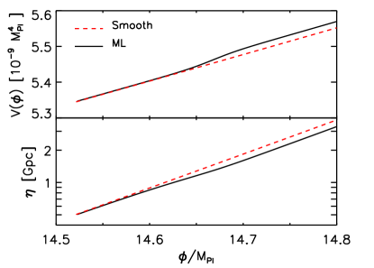
Figure 1: Upper panel: inflationary potential with a step from Eq. (3) with parameters that maximize the WMAP5 likelihood (ML, black/solid) and an $m^{2}\phi^{2}$ potential that matches the WMAP5 normalization (smooth, red/dashed). Lower panel: conformal time to the end of inflation as a function of the value of the field.

An example of such a case is a step in the inflaton potential of the form $V(\phi)=m^{2}_{\rm eff}(\phi)\phi^{2}/2$, where the effective mass of the inflaton potential is given by Adams:2001vc

$$m_{\rm eff}^{2}(\phi)=m^{2}\left[1+c\tanh\left(\frac{\phi-b}{d}\right)\right]\,.$$ (3)

This form for the potential has been shown to be a good description of large features in the temperature power spectrum at $\ell\sim 20-40$ tentatively seen in the WMAP data Covi:2006ci ; Hamann:2007pa . The maximum likelihood (ML) parameters values for WMAP5 are $b=14.668$, $c=1.505\times 10^{-3}$, $d=0.02705$ and $m=7.126\times 10^{-6}$ Mortonson:2009qv . The potential for this choice of parameters is shown in Fig. 1 (upper panel). For comparison we also show the best fit smooth model ($c=0$) with $m=7.12\times 10^{-6}$. Since it will be convenient to express results in terms of physical scale instead of field value, we also show in the lower panel the relationship to the conformal time to the end of inflation $\eta=\int^{t_{\rm end}}_{t}dt^{\prime}/a.$ Note that $\eta$ is defined to be positive during inflation. The two models have comparable power at wavenumbers $k\sim\eta^{-1}\sim 0.02$ Mpc^-1.

The slow-roll parameters for these models as a function of $\eta$ are shown in Fig. 2. Notice that $\epsilon_{H}$ remains small in the ML model though its value changes fractionally by order unity. On the other hand, $\eta_{H}$ is of order unity and $\delta_{2}$ is greater than unity in amplitude in this model around $\eta\sim 1$ Gpc when the inflaton rolls across the feature.

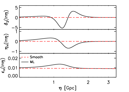
Figure 2: Slow-roll parameters $\epsilon_{H}$, $\eta_{H}$ and $\delta_{2}$ for the two models of Fig. 1: ML step model (black/solid) and smooth model (red/dashed).

II.1 Exact Relations

It is useful to begin by examining the exact equations and solutions. The exact equation of motion of each $k$-mode of the inflaton field is given by

$${d^{2}u_{k}\over d\eta^{2}}+(k^{2}-{1\over z}{d^{2}z\over d\eta^{2}})u_{k}=0\,,$$ (4)

where

$$z={f\over 2\pi\eta}\,,\quad f=2\pi{{\dot{\phi}}a\eta\over H}\,.$$ (5)

The field amplitude is related to the curvature power spectrum by

$$\Delta^{2}_{\cal R}(k)={k^{3}\over 2\pi^{2}}\lim_{k\eta\rightarrow 0}\left|\frac{u_{k}}{z}\right|^{2}\,.$$ (6)

Following Stewart:2001cd , we begin by transforming the field equation into dimensionless variables $y=\sqrt{2k}u_{k}$, $x=k\eta$

$${d^{2}y\over dx^{2}}+\left(1-{2\over x^{2}}\right)y={g(\ln x)\over x^{2}}y\,,$$ (7)

where

$$g={f^{\prime\prime}-3f^{\prime}\over f}\,.$$ (8)

Primes here and throughout are derivatives with respect to $\ln\eta$.

The functions $f$ and $g$ carry information about deviations from perfect slow roll $\epsilon_{H}=0$, $\eta_{H}=0$ and $\delta_{2}=0$. Specifically, without assuming that these three parameters are small or slowly varying

$$f^{2} = 8\pi^{2}{\epsilon_{H}\over H^{2}}(aH\eta)^{2}\,,$$

$${f^{\prime}\over f} = -aH\eta(\epsilon_{H}-\eta_{H})+(1-aH\eta)\,,$$

$${f^{\prime\prime}\over f} = 3{f^{\prime}\over f}+2[(aH\eta)^{2}-1]$$

$$+(aH\eta)^{2}[2\epsilon_{H}-3\eta_{H}+2\epsilon_{H}^{2}-4\eta_{H}\epsilon_{H}+\delta_{2}]\,,$$

and the dynamics of the slow-roll parameters themselves are given by

$${d\epsilon_{H}\over d\ln a} = 2\epsilon_{H}(\epsilon_{H}-\eta_{H})\,,$$ (10)

$${d\eta_{H}\over d\ln a} = \epsilon_{H}\eta_{H}+\eta_{H}^{2}-\delta_{2}\,.$$ (11)

Moreover, these quantities are related to the inflaton potential by

$$({V_{,\phi}\over V})^{2} = 2\epsilon_{H}{(1-\eta_{H}/3)^{2}\over(1-\epsilon_{H}/3)^{2}}\,,$$

$${V_{,\phi\phi}\over V} = {\epsilon_{H}+\eta_{H}-\delta_{2}/3\over 1-\epsilon_{H}/3}\,,$$ (12)

which in the limit of small and nearly constant $\eta_{H}$, $\epsilon_{H}$ return the ordinary slow roll relations.

In general, there is no way to directly express the source function $g$ in terms of the potential without approximation. Here we want to consider a situation where the feature in the potential is not large enough to interrupt inflation and hence $\epsilon_{H}\ll 1$, but is sufficiently large to make $\eta_{H}$ of order unity for less than an $e$-fold. By virtue of Eq. (11), $|\delta_{2}|\gg 1$ during this time. This differs from other treatments which assume $|\eta_{H}|\ll 1$ and by virtue of Eq. (10) a nearly constant $\epsilon_{H}$ Stewart:2001cd .

Even under these generalized assumptions there are some terms in $\eta_{H}$ and $\delta_{2}$ that can be neglected. For example, even if $\eta_{H}$ is not small, it suffices to take

$$aH\eta-1=\epsilon_{H}+\epsilon_{H}{\cal O}(\eta_{H})\,.$$ (13)

This expression preserves the ordinary slow roll relations when $|\eta_{H}|\ll 1$. When $\eta_{H}$ is not small, this quantity remains of order $\epsilon_{H}$ and so is negligible compared with bare $\eta_{H}$ and $\delta_{2}$ terms. Hence this approximation suffices everywhere.

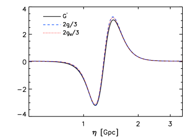
Figure 3: Source functions for the deviations from slow roll used in the GSR approximations: $2g/3$, $2g_{V}/3$ and $G^{\prime}$ (see §II.3) for the maximum likelihood model. To good approximation $g=g_{V}$ which directly relates the source function to features in the inflaton potential. Likewise $G^{\prime}\approx 2g_{V}/3$ and is most simply related to the curvature power spectrum for large deviations.

Following this logic, we obtain

$$g=g_{V}+\epsilon_{H}{\cal O}(\epsilon_{H},\eta_{H},\delta_{2})\,,$$ (14)

where $g_{V}$ is directly related to the potential

$$g_{V} \equiv {9\over 2}({V_{,\phi}\over V})^{2}-3{V_{,\phi\phi}\over V}$$ (15)

$$= 6\epsilon_{H}-3\eta_{H}+\delta_{2}+\epsilon_{H}{\cal O}(\epsilon_{H},\eta_{H},\delta_{2})\,.$$

As shown in Fig. 3, this relationship between the source function $g$ and features in the potential $V$ holds even for the ML step potential. Thus, if we can express the functional relationship between $g$ and the curvature power spectrum that is valid for large $g$ we can use features in the power spectrum to directly constrain features in the inflaton potential.

To determine this relation note that in the $x$ and $y$ variables the curvature is ${\cal R}={xy/f},$ and its power spectrum is $\Delta^{2}_{\cal R}(k)=\lim_{x\ll 1}\left|{\cal R}\right|^{2}.$ The LHS of Eq. (7) is simply the equation for scale invariant perfect slow roll and is solved by

$$y_{0}(x)=\left(1+{i\over x}\right)e^{ix}\,,$$ (16)

and its complex conjugate $y_{0}^{*}(x)$. An exact, albeit formal solution to the field equation can be constructed with the Green function technique Stewart:2001cd

$$y(x)=y_{0}(x)-\int_{x}^{\infty}{du\over u^{2}}g(\ln u)y(u){\rm Im}[y_{0}^{*}(u)y_{0}(x)]\,.$$ (17)

The solution is only formal since $y$ appears on both the left and right hand side of the equation. The corresponding formal solution for the curvature power spectrum can be made more explicit by parameterizing the source $y(u)$ as

$$y(u)=F_{\rm R}(u){\rm Re}[y_{0}(u)]+iF_{\rm I}(u){\rm Im}[y_{0}(u)]$$ (18)

so that

$$\lim_{x\ll 1}{(xy)} = i-{i\over 3}\int_{x}^{\infty}{du\over u}{x^{3}\over u^{3}}F_{\rm I}(u)g(\ln u)$$

$$+{i\over 3}\int_{x}^{\infty}{du\over u}W(u)F_{\rm I}(u)g(\ln u)$$

$$+{1\over 3}\int_{x}^{\infty}{du\over u}X(u)F_{\rm R}(u)g(\ln u)$$

$$+{x^{3}\over 9}\int_{x}^{\infty}{du\over u}W(u)F_{\rm R}(u)g(\ln u)+{\cal O}(x^{2})\,,$$

where

$$W(u) \equiv -{3\over u}{\rm Im}[y_{0}(u)]{\rm Re}[y_{0}(u)]$$

$$= {3\sin(2u)\over 2u^{3}}-{3\cos 2u\over u^{2}}-{3\sin(2u)\over 2u}\,,$$

$$X(u) \equiv {3\over u}{\rm Re}[y_{0}(u)]{\rm Re}[y_{0}(u)]$$ (20)

$$= -{3\cos(2u)\over 2u^{3}}-{3\sin(2u)\over u^{2}}$$

$$+{3\cos(2u)\over 2u}+{3\over 2u^{3}}(1+u^{2})\,.$$

Note that $\lim_{u\rightarrow 0}W(u)=1$ and $\lim_{u\rightarrow 0}X(u)=u^{3}/3$ and we have utilized the fact that

$${\rm Im}[y_{0}(u)]{\rm Im}[y_{0}(u)]={1+{1\over u^{2}}}-{u\over 3}X(u)$$ (21)

goes to $1/u^{2}$ in the limit $u\rightarrow 0$.

Finally, the curvature power spectrum becomes

$$\Delta^{2}_{\cal R}(k)=\lim_{x\ll 1}x^{2}{[{\rm Im}(y)]^{2}+[{\rm Re}(y)]^{2}\over f^{2}}\,,$$ (22)

with $y$ given by Eq. (II.1).

II.2 GSR for Small Deviations

The fundamental assumption in GSR is that one recovers a good solution by setting $F_{\rm I}(u)=F_{\rm R}(u)=1$ in the formal solution for the field fluctuations in Eq. (II.1). Equivalently, $y(u)\rightarrow y_{0}(u)$ in the source term on the RHS of Eq. (7). Note that this does not necessarily require that $g$ itself is everywhere much less than unity. For example, modes that encounter a strong variation in $g$ while deep inside the horizon do not retain any imprint of the variation and hence the GSR approximation correctly describes the curvature they induce.

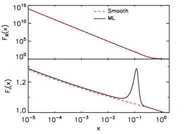
Figure 4: Ratio of field solution $y$ to the scale invariant approximation $y_{0}$. Upper panel: real part $F_{\rm R}$ for a smooth case (red/dashed line), and for the maximum likelihood model (black/solid line), both at $k=10^{-4}$ Mpc^-1. Lower panel: imaginary part $F_{\rm I}$ for the same models.

In Fig. 4, we show an example of $F_{\rm I}$ and $F_{\rm R}$ for a mode with $k=10^{-4}$ Mpc^-1 for both the ML and smooth models. For the ML model, this mode is larger than the horizon when the inflaton crosses the feature. Note that even in the smooth model, the two functions deviate substantially from unity at $x\ll 1$. In fact, they continue to increase indefinitely after horizon crossing and $F_{\rm R}\propto x^{-3}$ diverges to compensate for $|{\rm Re}(y_{0})|\propto x^{2}$. For the ML model, even $F_{\rm I}$ deviates strongly from unity during the crossing of the feature at $x\sim 0.1$.

The impact that these deviations have on the curvature spectrum can be better understood by reexpressing the various contributions in a more compact form. First note that

$$\lim_{x\ll 1}{x^{3}\over 3}\int_{x}^{\infty}{du\over u}u^{-3}g(\ln u) = -{1\over 3}\left({f^{\prime}\over f}\right)\,,$$ (23)

and so Eq. (II.1) becomes

$$\lim_{x\ll 1}{|{\cal R}_{\rm GSRS}|}={1\over f}\left[1+{1\over 3}{f^{\prime}\over f}+{1\over 3}\int_{x}^{\infty}{du\over u}W(u)g(\ln u)\right]\,,$$ (24)

where note that we have dropped the Re($xy$) contribution since it adds in quadrature to the power spectrum and hence is second order in $g$. We call this the “GSRS” approximation for the curvature power spectrum $\Delta_{\cal R}^{2}=\lim_{x\ll 1}|{\cal R}_{\rm GSRS}|^{2}$ given its validity for small fluctuations in the field solution from $y\rightarrow y_{0}$.

The choice of $x$ is somewhat problematic Stewart:2001cd . From Fig. 4, we see that taking $x$ too small will cause spurious effects since $F_{\rm I}$ increases as $x$ decreases. On the other hand, $x$ cannot be chosen to be too large for the ML model since it will cause some $k$ modes to have their curvature calculated when the inflaton is crossing the feature. Moreover, if $x$ is set to be some fixed conformal time during inflation $\eta_{\rm min}$, then it will vary with $k$.

We illustrate these problems in Fig. 5. For $\eta_{\rm min}=10^{-1}$ Mpc (upper panel), GSRS underpredicts power at low $k$ for the smooth model and overpredicts it for the ML model. Agreement for the smooth model is improved by choosing $x=10^{-2}$, i.e. nearer to horizon crossing (cf. Appendix for variants that take $x\approx 1$). On the other hand, the agreement for the ML model becomes worse and has a spurious feature at $k\sim 10^{-5}$ Mpc^-1 where the inflaton is crossing the feature at $x=10^{-2}$. In the next section, we shall examine the origin of the deviations from the exact solution and how a variant of the GSR approximation can fix most of them.

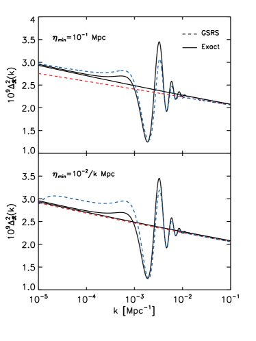
Figure 5: GSRS approximation to the curvature power spectrum (dashed lines) compared to the exact solution (solid lines) for a choice of $\eta_{\rm min}=10^{-1}$ Mpc (upper panel) and $\eta_{\rm min}=10^{-2}/k$ Mpc (lower panel). The ML model is shown in blue and the smooth model in red for GSRS.

II.3 GSR for Large Deviations

When considering large deviations from scale invariance, either due to sharp features in the potential or due to extending the calculation for many $e$-folds after horizon crossing, the first qualitative problem with the GSRS approximation of Eq. (24) is that it represents a linearized expansion for a correction that is not necessarily small. When the correction becomes large, ${\cal R}_{\rm GSRS}$ can pass through zero leaving nodes in the spectrum. While this is not strictly a problem for the ML model, it is better to have a more robust implementation of GSR for likelihood searches over the parameter space.

We can finesse this problem by replacing the linearized expansion $1+x$ by $e^{x}$ and write the power spectrum in the form

$$\ln\Delta_{\cal R}^{2}(k)=G(\ln\eta_{\rm min})+{2\over 3}\int_{\eta_{\rm min}}^{\infty}{d\eta\over\eta}W(k\eta)g(\ln\eta)\,,$$ (25)

where

$$G(\ln\eta)=\ln\left({1\over f^{2}}\right)+{2\over 3}{f^{\prime}\over f}\,.\\$$ (26)

This procedure returns the correct result at first order since $g$ and $f^{\prime}/f$ are both first order in the slow-roll parameters (see Eq. (II.1)). We shall see below that it can be further modified to match the fully non-linear result for superhorizon modes.

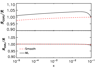
Figure 6: Curvature evolution after horizon crossing in the GSRS (upper panel) and GSRL (lower panel) approximations, both normalized to the exact solution. The ML model (black/solid line) and smooth model (red/dashed line) are both shown at $k=10^{-4}$ Mpc^-1.

The more fundamental problem with GSRS is the deviation of the true solution $y$ from the scale invariant solution $y_{0}$ when the mode is outside the horizon (see Fig. 4). The origin of this problem is that the exact solution requires the curvature ${\cal R}=xy/f$ to be constant outside the horizon, independently of how strongly $f$ evolves. Thus, if $f$ is allowed to vary significantly, either due to the large number of $e$-folds that have intervened since horizon crossing or due to a feature in the potential, then $y$ must follow suit and deviate from $y_{0}$ breaking the GSRS approximation.

Fig. 6 (upper panel) illustrates this problem. Even for the smooth model, the curvature is increasingly underestimated as $x\rightarrow 0$ . With the ML model, the crossing of the feature induces an error of the opposite sign. For $x\sim 10^{-5}$ these problems fortuitously cancel but not for any fundamental or model independent reason.

Given this problem, GSRS actually works better than one might naively expect. For example at $k=10^{-4}$ Mpc^-1, even though $F_{\rm I}\sim 1.28$ at $x=10^{-5}$, the GSRS approximation gives a $\sim 2.5\%$ difference in the curvature and a $\sim 5\%$ difference in the power spectrum with the exact solution for the smooth model instead of the $28\%$ and the $64\%$ differences one might guess. The main contribution to the GSRS correction from scale invariance is given by the integral term in Eq. (24), which is $\sim 0.25$ for the smooth case. Given that $F_{I}$ is a linear function in $\ln\eta$ and $g$ is slowly varying, we can approximate enhancement due to $F_{I}$ of the integral term by its average interval ($\sim 1.14$). With this rough estimate we obtain an approximately $(1+0.25)^{2}/(1+0.25\times 1.14)^{2}\sim 5-6\%$ error in power in agreement with the power spectrum result in Fig. 5.

Furthermore although $F_{\rm R}$ diverges as $x^{-3}$ in Fig. 4, the contribution to the power spectrum of the real part of $y$ remains small. Its absence in the GSRS approximation produces a negligible effect for modes that are larger than the horizon when the inflaton crosses the feature. The integrands for the real contribution contain either the function $X$, which peaks at horizon crossing $x\sim 1$, or $x^{3}W(u)$ which is likewise suppressed at $x\ll 1$. The correction adds in quadrature to the imaginary part and so it is intrinsically a second order correction (see §II.5). For $k=10^{-4}$ Mpc^-1 its contribution to the power spectrum is $0.08\%$ of the power spectrum in the ML model. The fact that integrals over the deviation of $y$ from $y_{0}$ can remain small even when neither $g$ nor the maximum of $y-y_{0}$ is small is crucial to explaining why the GSR approximation works so well and why we can extend GSRS with small, controlled corrections.

Nonetheless these problems with GSRS are significant and exacerbated by the presence of sharp features in the potential. The fundamental problem with GSRS is that its results depend on an arbitrarily chosen value of $x\ll 1$, i.e. ${\cal R}$ is not strictly constant in this regime. Phrased in terms of Eq. (26) the problem is that $g$ is not directly related to $G$ but rather

$${2\over 3}g=G^{\prime}+{2\over 3}\left({f^{\prime}\over f}\right)^{2}\,,$$ (27)

where

$$G^{\prime}={dG\over d\ln\eta}={2\over 3}({f^{\prime\prime}\over f}-3{f^{\prime}\over f}-{f^{\prime 2}\over f^{2}})\,.$$ (28)

In GSRS, replacing $g$ with $3G^{\prime}/2$ amounts to a second order change in the source function. In fact even for the ML step function this change is a small fractional change of the source everywhere in $\ln\eta$: it is small as the inflaton rolls past the feature since $|f^{\prime\prime}/f|\gg(f^{\prime}/f)^{2}$ and it is small before and after this time since $|f^{\prime}/f|\ll 1$. In terms of the slow-roll parameters, this replacement is a good approximation if $\eta_{H}^{2}\sim O(1)$ only where $|\delta_{2}|\gg 1$ and $g\approx\delta_{2}$ (see Eqs. (14) and (15)).

$$G^{\prime}={2\over 3}g+{2\over 3}\eta_{H}^{2}+\epsilon_{H}{\cal O}(\epsilon_{H},\eta_{H},\delta_{2})$$ (29)

Moreover $G^{\prime}\approx 2g_{V}/3$ and remains directly relatable to the inflaton potential through Eq. (15). For comparison we show all three versions of the GSR source function in Fig. 3.

Nonetheless, the replacement can have a substantial effect on the curvature once the source is integrated over $\ln\eta$ because the difference is a positive definite term in the integral. Moreover, this cumulative effect is exactly what is needed to recover the required superhorizon behavior. Replacing $2g/3\rightarrow G^{\prime}$ in the power spectrum expression, we obtain Kadota:2005hv

$$\ln\Delta_{\cal R}^{2}(k)=G(\ln\eta_{\rm min})+\int_{\eta_{\rm min}}^{\infty}{d\eta\over\eta}W(k\eta)G^{\prime}(\ln\eta)\,,$$ (30)

which we call the GSRL approximation. The field solution corresponding to this approximation, valid for $x\ll 1$, is given by

$$\lim_{x\ll 1}{|xy|}=\exp\left[{1\over 3}{f^{\prime}\over f}+{1\over 2}\int_{x}^{\infty}{du\over u}W(u)G^{\prime}(\ln u)\right]\,.$$ (31)

Now any variation in $f$ while the mode is outside the horizon and $W(k\eta)\approx 1$ integrates away and gives the same result as if $\ln\eta_{\rm min}$ were set to be right after horizon crossing for the mode in question. This can be seen more clearly by integrating Eq. (30) by parts Kadota:2005hv

$$\ln\Delta_{\cal R}^{2}(k)=-\int_{\eta_{\rm min}}^{\infty}{d\eta\over\eta}W^{\prime}(k\eta)G(\ln\eta)\,.$$ (32)

Since $-\int_{0}^{\infty}d\ln xW^{\prime}(x)=1$ and $\lim_{x\rightarrow 0}W^{\prime}(x)\rightarrow 0$, the curvature spectrum does not depend on the evolution of $f$ outside the horizon. Moreover, the integral gets its contribution near $x\sim 1$ so for smooth functions $G(\ln\eta)$ we recover the slow roll expectation that

$$\ln\Delta_{\cal R}^{2}(k)\approx G(\ln\eta)\Big{|}_{k\eta\approx 1}\,.$$ (33)

If the slow-roll parameters are all small then the leading order term in Eq. (33) returns the familiar expression for the curvature spectrum $\Delta_{\cal R}^{2}\approx f^{-2}\approx H^{2}/8\pi^{2}\epsilon_{H}$ at $k\eta\approx 1$. Choe et al. Choe:2004zg showed that Eq. (32) is correct up to second order in $g$ for $k\eta\ll 1$. Here we show that it is correct for arbitrary variations in $f$ and $g$ outside the horizon.

The superhorizon curvature evolution for $k=10^{-4}$ Mpc^-1 corresponding to the GSRL approximation is shown in Fig. 6 (lower panel). In the $x\ll 1$ domain of applicability of Eq. (31), the curvature is now appropriately constant for both the ML and smooth models. The net result is that the curvature power spectrum shown in Fig. 7 is now a good match to the exact solution for low $k$.

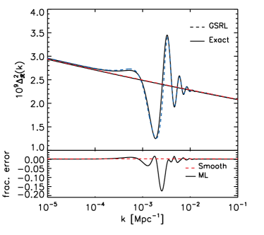
Figure 7: GSRL approximation to the curvature power spectrum. Upper panel: approximation compared with the exact solution (solid lines) for the maximum likelihood model. Lower panel: fractional error between the approximation and the exact solution.

II.4 Power Spectrum Features

We now turn to issues related to the response of the field and curvature for $k$ modes that are inside the horizon when the inflaton rolls across the feature. Fig. 7 shows that the GSRL approximation works remarkably well for the ML model despite the fact that the power spectrum changes by order unity there. The main problem is a $\sim 10-20\%$ deficit of power for a small range in $k$ near the sharp rise between the trough and the peak.

In Fig. 8, we show the deviation of the exact solution $y$ from the scale invariant $y_{0}$ that is at the heart of the GSR approximation. The three modes shown, $k_{\rm dip}=1.8\times 10^{-3}$ Mpc^-1, $k_{\rm node}=2.5\times 10^{-3}$ Mpc^-1, $k_{\rm bump}=3.2\times 10^{-3}$ Mpc^-1, correspond to the first dip, node and bump in the power spectrum of the ML model.

The first thing to note is that for higher $k$, the inflaton crosses the feature at increasing $x$ where the deviations of $y$ from $y_{0}$ actually decrease. Hence the fundamental validity of the GSR approximation actually improves for subhorizon modes. Combined with the GSRL approximation that enforces the correct result at $x\ll 1$, this makes the approximation well behaved nearly everywhere.

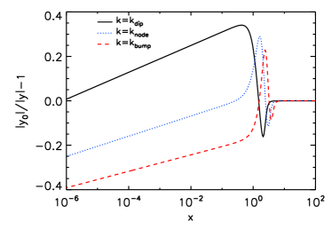
Figure 8: Fractional difference between $|y_{0}|$ and $|y|$ for the ML model at $k$ values at the dip, node and bump of the feature in the power spectrum (see text).

The small deviations from GSRL appear for modes that cross the horizon right around the time that the inflaton crosses the feature. It is important to note that the step potential actually provides two temporal features in $g$ or $G^{\prime}$ displayed in Fig. 3. Each mode first crosses a positive feature at high $\eta$ and $x$ and then goes through a nearly equal and opposite negative feature. The end result for the field amplitude or curvature is an interference pattern of contributions from both temporal features. For example, the peak in power is due to the constructive interference between a positive response to the positive feature and a negative response to the negative feature. This suggests that one problem with the GSRL approach is that it does not account for the deviation of the field $y$ from $y_{0}$ that accumulates through passing the positive temporal feature when considering how the field goes through the negative feature. This is intrinsically a non-linear effect.

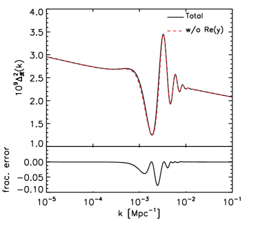
Figure 9: Contribution of the real part of the $y$ field to the curvature power spectrum. Upper panel: spectrum with and without the real part. Lower panel: fractional error between the two solutions.

The final thing to note is that, since $g$ and $G^{\prime}$ are of order unity as these modes exit the horizon, the real part of the field solution is not negligible. Moreover, it contributes a positive definite piece to the power spectrum. In Fig. 9, we show the result of dropping the real part from the exact solution. Note that the fractional error induced by dropping the real part looks much like the GSRL error in Fig. 7 but with $\sim 1/2$ the amplitude.

II.5 Iterative GSR Correction

The good agreement between GSRL and the exact solution even in the presence of large deviations in the curvature spectrum suggests that a small higher order correction may further improve the accuracy. Moreover, the analysis in the previous section implies that there are two sources of error: the omission of the field response from inside the horizon $x>1$ when computing the response of the field to features at horizon crossing $x\sim 1$ and the dropping of the real part of the field solution.

Both of these contributions come in at second order in the GSR approximation. All first order GSR variants involve the replacement of the true field solution $y$ with the scale invariant solution $y_{0}$ in Eq. (7). This replacement can be iterated with successively better approximations to $y$. We begin with the GSRS approximation of replacing $y\rightarrow y_{0}$ to obtain the first order solution $y_{1}$. We then replace $y\rightarrow y_{1}$ in the source to obtain a second order solution $y_{2}$, etc.

We show the fractional error between the iterative solutions and the exact solution for $k=k_{\rm node}$ in Fig. 10, where the error in GSRL is roughly maximized. As in the first order GSRS approach, the accuracy depends on the arbitrary choice of $x=k\eta_{\rm min}$ when the curvature is computed. The number of iterations required for a given accuracy increases with decreasing $x$. We show the curvature spectrum in Fig. 11 for the same two choice of $\eta_{\rm min}=10^{-1}$ Mpc (upper panel) and $\eta_{\rm min}=10^{-2}/k$ Mpc (lower panel) as in Fig. 5. Note that in both cases, the result has converged at the $0.5\%$ percent level or better to the exact solution within three iterations.

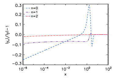
Figure 10: Fractional difference between the exact ($y$) and $n$th order iterative solutions ($y_{n}$) for the ML model at $k=k_{\rm node}$ where the errors in the GSRL approximation are maximized.

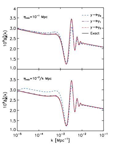
Figure 11: Curvature power spectrum in the GSRS approximation for $\eta_{\rm min}=10^{-1}$ Mpc (upper panel) and $\eta_{\rm min}=10^{-2}/k$ Mpc (lower panel) when $y\rightarrow y_{n}$ in the GSRS source compared to the exact solution.

Unfortunately the iterative GSRS approach is not of practical use in that each iteration requires essentially the same effort as a single solution of the exact approach. On the other hand, rapid convergence in the iterative GSRS approach suggests that a nonlinear correction to GSRL based on a second order expansion might suffice. A second order GSRL approach differs conceptually from the iterative GSRS approach in that it is formally an expansion in $g$ where in our case $|g|\ll 1$ is not satisfied. The iterative GSRS approach is exact in $g$ but expands in $y-y_{0}$. What makes a second order GSRL approach feasible is that the critical elements involve time integrals over $g$ which can be small even if $g$ is not everywhere small.

Our strategy for devising a non-linear correction to GSRL is to choose a form that reproduces GSRL at first order in $g$, is exact at second order in $g$, is simple to relate to the inflaton potential, and finally is well controlled at large values of $g$. The second order in $g$ expressions for the curvature are explicitly given in Choe:2004zg and come about by both iterating the integral solution in Eq. (II.1) and dropping higher order terms. Our criteria are satisfied by

$$\Delta^{2}_{\cal R}=\Delta^{2}_{\cal R}|_{\rm GSRL}\left\{[1+{1\over 4}I_{1}^{2}(k)+{1\over 2}I_{2}(k)]^{2}+{1\over 2}I_{1}^{2}(k)\right\}$$ (34)

where

$$I_{1}(k) = {1\over\sqrt{2}}\int_{0}^{\infty}{d\eta\over\eta}G^{\prime}(\ln\eta)X(k\eta)\,,$$

$$I_{2}(k) = -4\int_{0}^{\infty}{du\over u}[X+{1\over 3}X^{\prime}]{f^{\prime}\over f}F(u)\,,$$ (35)

with

$$F(u)=\int_{u}^{\infty}{dv\over v^{2}}{f^{\prime}\over f}\,.$$ (36)

We call this the GSRL2 approximation. In the Appendix we discuss alternate forms Choe:2004zg .

In the GSRL2 approach, $I_{1}$ corrections come half from the first order calculation of the real part of the field and half from iterating the imaginary part to second order. In Fig. 12 we show $I_{1}^{2}$ and $I_{2}$ for the ML model. Note that $I_{1}^{2}$ dominates the correction to the net power as it always enhances power, while $I_{2}$ is both smaller and oscillates in its correction. Furthermore, both $|I_{1}^{2}|\ll 1$ and $|I_{2}|\ll 1$ for the ML model which justifies a second order approach to these corrections. The GSRL2 correction can be taken to be $\{1+I_{1}^{2}+I_{2}\}$ in this limit.

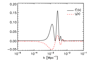
Figure 12: Second order GSRL2 power spectrum correction functions $I_{1}^{2}$ and $I_{2}$ for the ML model.

We show in Fig. 13 how the GSRL2 corrections reduce the power spectrum errors of GSRL in Fig. 7 for the ML model. For the full GSRL2 expression the power spectrum errors are reduced from the $10-20\%$ level to the $\lesssim 4\%$ level. We show that the GSRL2 approximation remains remarkably accurate for substantially larger features in the Appendix.

Moreover, the errors are oscillatory and their observable consequence in the CMB is further reduced by projection. The temperature and polarization power spectra are shown in Fig. 14 and 15 and the errors are $\lesssim 0.5\%$ and $\lesssim 2\%$ for the respective spectra.

Given the intrinsic smallness of $I_{2}$ and its oscillatory nature, the most important correction comes from the positive definite $I_{1}$ piece. Note that it is a single integral over the same $G^{\prime}$ function as in the linear case. Thus, $I_{1}$ corrections simply generalize the GSRL mapping between $G^{\prime}$ and curvature in a manner that is equally simple to calculate. $I_{2}$ on the other hand is more complicated and involves a non-trivial double integral with a different dependence on the inflaton potential.

We also show in Figs. 13-15 the results for the GSRL2 expression with $I_{2}$ omitted. While the curvature power spectrum errors increase slightly to $\sim 5\%$, the temperature power spectrum errors at $\lesssim 2\%$ are still well below the $\sim 20\%$ cosmic variance errors per $\ell$ at $\ell\sim 30$. They are even sufficient for the cosmic variance limit of coherent deviations across the full range of the feature ($20\lesssim\ell\lesssim 40$) $20\%/\sqrt{20}\sim 4-5\%$ in the ML case. The polarization spectrum has slightly larger errors due to the reduction of projection effects but still satisfies these cosmic variance based criteria.

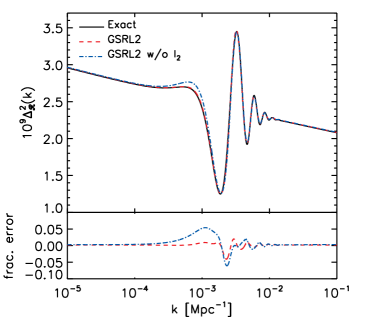
Figure 13: GSRL2 approximation to the curvature power spectrum. Upper panel: approximation of Eq. (34) (red/dashed line) compared to the exact solution (black/solid line). We also show the GSRL2 approximation omitting the $I_{2}$ term (blue/dashed-dotted line). Lower panel: fractional error between these GSRL2 approximations and the exact solution.

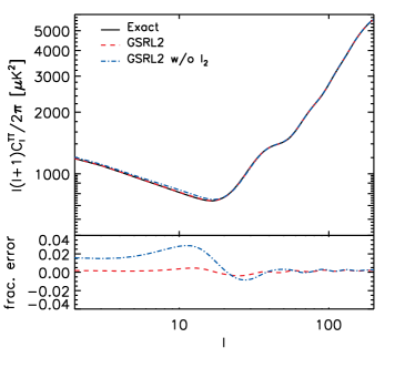
Figure 14: GSRL2 approximation to the CMB temperature power spectrum. Upper panel: approximation (red/dashed line) compared to the exact solution (black/solid line). We also show the GSRL2 approximation omitting the $I_{2}$ term (blue/dashed-dotted line). Lower panel: fractional error between the GSRL2 approximations and the exact solution.

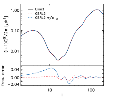
Figure 15: GSRL2 approximation to the CMB $E$-mode polarization power spectrum. The same as in Fig. 14.

III Applications

In the previous section, we have shown that a particular variant of the GSR approximation which we call GSRL2 provides a non-linear mapping between $G^{\prime}$ and the curvature power spectrum. $G^{\prime}$ quantifies the deviations from slow roll in the background and moreover is to good approximation directly related to the inflaton potential. These relations remain true even when the slow-roll parameter $\eta_{H}$ is not small compared to unity for a fraction of an $e$-fold.

This relationship is useful for considering inflation-model independent constraints on the inflaton potential. It is likewise useful for inverse or model building approaches of finding inflaton potential classes that might fit some observed feature in the data. We intend to further explore these applications in a future work.

Here as a simple example let us consider a potential that differs qualitatively from the step potential but shares similar observable properties through $G^{\prime}$: $V(\phi)=m^{2}_{\rm eff}\phi^{2}/2$ where the effective mass of the inflaton now has a transient perturbation instead of a step

$$m^{2}_{\rm eff}=m^{2}\left[1+Ae^{-(\phi-b)^{2}/(2\sigma^{2})}(\phi-b)\right]$$ (37)

In Fig. 16 we show the potential for the choice of parameters $b=14.655$, $A=0.0285$, $\sigma=0.025$, and $m=7.126\times 10^{-6}$ (upper panel) and we also show $G^{\prime}$ in the lower panel. For comparison we show the smooth case $A=0$. Comparison with Figs. 1 and 2 shows that this potential, which has a bump and a dip instead of a step, produces a similar main feature in $G^{\prime}$ but has additional lower amplitude secondary features.

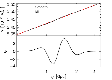
Figure 16: Alternate inflationary model with a perturbation in the mass. Upper panel: comparison of potential in Eq. (37) (black/solid line) and the smooth potential (red/dashed line). Lower panel: source function of the deviation from slow roll $G^{\prime}$ for the same models.

In Fig. 17 we compare the GSRL2 approximation with and without the double integral $I_{2}$ term compared to the exact solution. Notice that GSRL2 performs equally well for this very different sharp potential feature. Furthermore, similarity in $G^{\prime}$ with the step potential carries over to similarity in the curvature power spectrum.

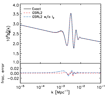
Figure 17: GSRL2 approximation to the alternate model of Fig. 16. Upper panel: approximation (red/dashed line) compared to the exact solution (black/solid line) for an effective mass given by Eq. (37). We also show the GSRL2 approximation with $I_{2}$ omitted (blue/dashed-dotted line). Lower panel: fractional error between GSRL2 approximations and the exact solution.

IV Discussion

We have shown that a variant of the generalized slow roll (GSR) approach remains percent level accurate at predicting order unity deviations in the observable CMB temperature and polarization power spectra from sharp potential features. Unlike other variants which explicitly require $|\eta_{H}|\ll 1$, and hence nearly constant $\epsilon_{H}$, our approach allows $\eta_{H}$ to be order unity, as long as it remains so for less than an $e$-fold, and hence $\epsilon_{H}$ to vary significantly. We have tested our GSR variant against a step function model that has been proposed to explain features in the CMB temperature power spectrum at $\ell\sim 20-40$.

Our analysis also shows that to good approximation a single function, $G^{\prime}(\ln\eta)$, controls the observable features in the curvature power spectrum even in the presence of large features. We have explicitly checked this relationship and the robustness of our approximation by constructing two different inflationary models with similar $G^{\prime}$.

Therefore observational constraints from the CMB can be mapped directly to constraints on this function independently of the model for inflation. Moreover, this function is also simply related to the slope and curvature of the inflaton potential in the same way that scalar tilt is related to the potential in ordinary slow roll $G^{\prime}\approx 3(V_{,\phi}/V)^{2}-2(V_{,\phi\phi}/V)$. These model independent constraints can then be simply interpreted in terms of the inflation potential. We intend to explore these applications in a future work.

Acknowledgments: We thank Hiranya Peiris for sharing code used to crosscheck exact results. We thank Michael Mortonson, Kendrick Smith and Bruce Winstein for useful conversations. This work was supported by the KICP under NSF contract PHY-0114422. WH was additionally supported by DOE contract DE-FG02-90ER-40560 and the Packard Foundation.

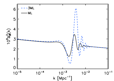
Figure 18: Curvature power spectrum for the ML and 3ML models.

Appendix A Other GSR Variants

In this Appendix, we compare various alternate forms discussed in the literature for the curvature power spectrum under the GSR approximation. We test these approximations against the GSRL and GSRL2 approximations of the main text for the ML model and a more extreme case with $c=3c_{\rm ML}=0.004515$ (with other parameters fixed) denoted 3ML (see Fig. 18). We begin by considering variants that are linear in the GSR approximation and then proceed to second order iterative approaches.

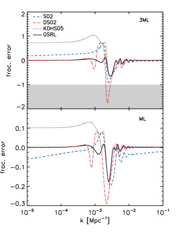
Figure 19: Fractional error in the curvature power spectrum for first order GSR variants for the ML model (lower) and the 3ML model (upper).

The first variant is the original linearized form of GSRS given in Stewart:2001cd (“S02”)

$$\Delta^{2}_{\cal R}(k)={1\over f^{2}}\left[1+{2\over 3}{f^{\prime}\over f}+{2\over 3}\int_{x}^{\infty}{du\over u}W(u)g(\ln u)\right]\,.$$ (38)

Like GSRS, this approximation depends on an arbitrary choice of $x$ but its impact is exacerbated by the linearization of the correction here. In Fig. 19 we show the fractional error in this approximation for $\eta_{\rm min}=10^{-1}$ Mpc. Note that because of the linearization, the curvature power spectrum can reach the unphysical negative regime (shaded region).

A second variant further exploits the relationship between the GSR source functions $f$, $f^{\prime}/f$ and $g$ and the potential through the slow-roll parameters (see Eq. (II.1)). By further assuming that $|\eta_{H}|\ll 1$, terms involving $V_{,\phi}/V$ can be taken to be constant and evaluated instead at horizon crossing $k=aH$ (see Eq. (10)). Finally by rewriting the change in $f^{\prime}/f$ as the integral of $(f^{\prime}/f)^{\prime}$, one obtains Dodelson:2001sh (“DS02”)

$$\Delta^{2}_{\cal R}(k) = {V\over 12\pi^{2}}\left({V\over V_{,\phi}}\right)^{2}\Big{\{}1+(3\alpha-{1\over 6})({V_{,\phi}\over V})^{2}|_{k=aH}$$ (39)

$$-2\int_{0}^{\infty}{du\over u}W_{\theta}(1,u){V_{,\phi\phi}\over V}\Big{\}},$$

where $\alpha\approx 0.73$ and with $\eta\approx 1/aH$, $u=k/aH$. Here

$$W_{\theta}(u_{*},u)=W(u)-\theta(u_{*}-u)$$ (40)

with the step function $\theta(x)=0$ for $x<0$ and $\theta(x)=1$ for $x\geq 0$. Note that $\lim_{u\rightarrow 0}W_{\theta}(1,u)=0$ and hence the function has weight only near horizon crossing at $u\approx 1$.

For cases like the ML and 3ML models where $\eta_{H}$ is neither small nor smoothly varying, these DS02 assumptions have both positive and negative consequences. They largely solve the problem for superhorizon modes discussed in §II.3 by extrapolating the evaluation of the potential terms from $k\eta\ll 1$ to $k\eta\sim 1$. On the other hand, a large $\eta_{H}$ means that $\epsilon_{H}$ evolves significantly. Artifacts of this evolution appear through the prefactor $(V/V_{,\phi})^{2}\propto 1/\epsilon_{H}$ in Eq. (39) most notably in the form of a spurious feature at $k\sim 10^{-3}$ Mpc^-1 in Fig. 19. Finally, like S02, DS02 does not guarantee a positive definite power spectrum.

A third variant is to replace $G^{\prime}$ with $2g_{V}/3$ in Eq. (30) so that the source directly reflects the potential Kadota:2005hv (“KDHS05”)

$$\ln\Delta_{\cal R}^{2}(k)=G(\ln\eta_{\rm min})+{2\over 3}\int_{\eta_{\rm min}}^{\infty}{d\eta\over\eta}W(k\eta)g_{V}\,.$$ (41)

As we have seen in §II.3, this approximation is actually fairly good locally in $\ln\eta$ and hence locally in $k$ around the feature. However the omission of $\eta_{H}^{2}$ terms causes a net error in the spectrum for $k$ modes that cross out of the horizon before the inflaton reaches the feature. Hence like the GSRS approximation, KDHS05 overpredicts power at low $k$ for the ML and 3ML models. Fig. 19 shows a choice with $\eta_{\rm min}=10^{-1}$ Mpc.

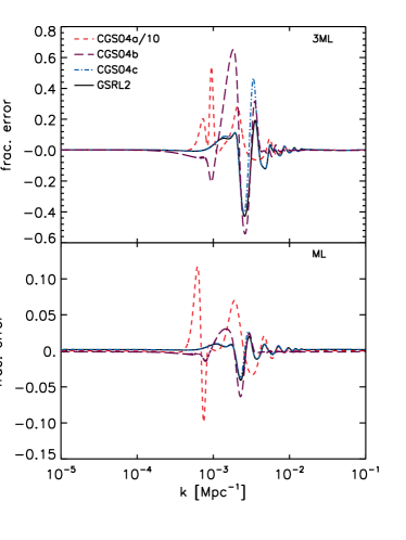
Figure 20: Fractional error in the curvature power spectrum for second order GSR variants (see text) for the ML model (lower panel) and the 3ML model (upper panel). Note that the error in CGS04a has been divided by a factor of 10 for plotting purposes.

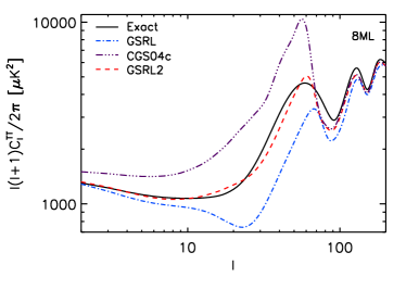
Figure 21: Temperature power spectrum for $c=8c_{\rm ML}$ (and the other parameters fixed). Note that even in this extreme, observationally unviable, case the temperature power spectrum has $<22\%$ errors everywhere for GSRL2 whereas the linear GSRL and CGS04c approximations substantially under and over predict power respectively.

We consider next second order GSR variants. The first variant Choe:2004zg begins with a second order approach as in GSRL2 but then further assumes that functions such as $f^{\prime}/f$ can be approximated by a Taylor expansion around $x_{*}$ to obtain (“CGS04a”)

$$\Delta^{2}_{\cal R} = {1\over f_{*}^{2}}\Big{\{}1-2\alpha_{*}{f^{\prime}_{*}\over f_{*}}+\left(-\alpha_{*}^{2}+{\pi^{2}\over 12}\right){f^{{}^{\prime\prime}}_{*}\over f_{*}}$$ (42)

$$+\left(3\alpha_{*}^{2}-4+{5\pi^{2}\over 12}\right)\left({f^{\prime}_{*}\over f_{*}}\right)^{2}$$

$$+\left[-{1\over 3}\alpha_{*}^{3}+{\pi^{2}\over 12}\alpha_{*}-{4\over 3}+{2\over 3}\zeta(3)\right]{f^{\prime\prime\prime}_{*}\over f_{*}}$$

$$+\left[3\alpha_{*}^{3}-8\alpha_{*}+{7\over 12}\pi^{2}\alpha_{*}+4-2\zeta(3)\right]{f^{\prime}_{*}f^{{}^{\prime\prime}}_{*}\over f^{2}_{*}}$$

$$+A\left({f^{\prime}_{*}\over f_{*}}\right)^{3}\Big{\}},$$

where $A=-4\alpha_{*}^{3}+16\alpha_{*}-5/3\pi^{2}\alpha_{*}-8+6\zeta(3)$, $\zeta$ is the Riemann zeta function, and $\alpha_{*}=\alpha-\ln(x_{*})$. This approach is essentially a standard slow roll approximation carried through to third order with the help of an exact solution for power law inflation. For the ML and 3ML models, applying this approximation leads to qualitatively incorrect results as one might expect. We show this variant in Fig. 20 with $x_{*}=1$.

A second variant attempts to retain both the generality of GSR and the evaluation of central terms at horizon crossing by implicitly modifying terms of order $(f^{\prime}/f)^{3}$ and higher when compared with GSRL2 Choe:2004zg (“CGS04b”)

$$\ln\Delta^{2}_{\cal R} = \ln\left({1\over f_{*}^{2}}\right)+{2\over 3}{f^{\prime}_{*}\over f_{*}}+{1\over 9}\left({f^{\prime}_{*}\over f_{*}}\right)^{2}$$

$$+{2\over 3}\int_{0}^{\infty}{du\over u}W_{\theta}(u_{*},u)g(u)$$

$$+{2\over 9}\left[\int_{0}^{\infty}{du\over u}X(u)g(u)\right]^{2}$$

$$-{2\over 3}\int_{0}^{\infty}{du\over u}X(u)g(u)\int_{u}^{\infty}{dv\over v^{2}}g(v)$$

$$-{2\over 3}\int_{0}^{\infty}{du\over u}X_{\theta}(u_{*},u)g(u)\int_{u}^{\infty}{dv\over v^{4}}g(v)\,,$$

where $W_{\theta}$ was given in Eq. (40) and

$$X_{\theta}(u_{*},u)=X(u)-{u^{3}\over 3}\theta(u_{*}-u)\,.$$ (44)

Here, the subscript $*$ denotes evaluation near horizon crossing. In Fig. 20 we show the result with $u_{*}=1$. Notably it performs worse than the first order GSRL approximation for the 3ML model.

Finally, the last variant considered takes Choe:2004zg (“CGS04c”)

$$\ln\Delta^{2}_{\cal R} = -\int_{0}^{\infty}{du\over u}W^{\prime}(u)\left[\ln\left({1\over f^{2}}\right)+{2\over 3}{f^{\prime}\over f}\right]$$

$$+2\left[\int_{0}^{\infty}{du\over u}\left(X(u)+{1\over 3}X^{\prime}(u)\right){f^{\prime}\over f}\right]^{2}$$

$$-4\int_{0}^{\infty}{du\over u}\left(X(u)+{1\over 3}X^{\prime}(u)\right){f^{\prime}\over f}F(u),$$

where $F(u)$ is given by Eq. (36). CGS04c is closely related to GSRL2 as integration by parts shows

$$\Delta^{2}_{\cal R}=\Delta^{2}_{\cal R}|_{\rm GSRL}e^{I_{1}^{2}(k)+I_{2}(k)}\,.$$ (46)

The main difference is that the second order corrections are exponentiated. This causes a noticeable overcorrection for the 3ML model when compared with GSRL2. In Fig. 20 we compare the three variants mentioned above.

Furthermore, in spite of the $20-40\%$ errors in the curvature power spectrum in the 3ML model for GSRL2, the CMB temperature power spectrum has only $1-2\%$ errors for $\ell\geq 20$ and a maximum of $<5\%$ errors at $\ell<20$. As discussed in the text, this level of error is sufficient for even cosmic variance limited measurements at the $\ell\lesssim 40$ multipoles of the feature. This reduction is due to the oscillatory nature of the curvature errors and projection effects in temperature.

In fact for even larger deviations GSRL2 still performs surprisingly well for the temperature power spectrum. In Fig. 21 we show the temperature power spectra for the GSRL2 approximation, and compare it with GSRL and CGS04c for a very extreme case with $c=8c_{\rm ML}$ (and the other parameters fixed). GSRL2 has a maximum of $22\%$ error in the temperature power spectrum and predicts qualitatively correct features. Finally, the dominant correction is from the term that is quadratic in $I_{1}$. The simplified GSRL2 form of

$$\Delta^{2}_{\cal R}=\Delta^{2}_{\cal R}|_{\rm GSRL}[1+{I_{1}^{2}(k)}]\,,$$ (47)

works nearly as well. Thus, the curvature power spectrum still depends only on $G^{\prime}$ to good approximation even in the most extreme case.

References

- (1) J. E. Lidsey et al., Rev. Mod. Phys. 69, 373 (1997), [arXiv:astro-ph/9508078].
- (2) WMAP, C. L. Bennett et al., Astrophys. J. Suppl. 148, 1 (2003), [arXiv:astro-ph/0302207].
- (3) WMAP, H. V. Peiris et al., Astrophys. J. Suppl. 148, 213 (2003), [arXiv:astro-ph/0302225].
- (4) L. Covi, J. Hamann, A. Melchiorri, A. Slosar and I. Sorbera, Phys. Rev. D74, 083509 (2006), [arXiv:astro-ph/0606452].
- (5) J. Hamann, L. Covi, A. Melchiorri and A. Slosar, Phys. Rev. D76, 023503 (2007), [arXiv:astro-ph/0701380].
- (6) M. J. Mortonson, C. Dvorkin, H. V. Peiris and W. Hu, Phys. Rev. D79, 103519 (2009), [arXiv:0903.4920].
- (7) C. Pahud, M. Kamionkowski and A. R. Liddle, Phys. Rev. D79, 083503 (2009), [arXiv:0807.0322].
- (8) M. Joy, A. Shafieloo, V. Sahni and A. A. Starobinsky, JCAP 0906, 028 (2009), [arXiv:0807.3334].
- (9) J. A. Adams, B. Cresswell and R. Easther, Phys. Rev. D64, 123514 (2001), [arXiv:astro-ph/0102236].
- (10) P. Hunt and S. Sarkar, Phys. Rev. D70, 103518 (2004), [arXiv:astro-ph/0408138].
- (11) S. Habib, A. Heinen, K. Heitmann, G. Jungman and C. Molina-Paris, Phys. Rev. D70, 083507 (2004), [arXiv:astro-ph/0406134].
- (12) M. Joy, E. D. Stewart, J.-O. Gong and H.-C. Lee, JCAP 0504, 012 (2005), [arXiv:astro-ph/0501659].
- (13) K. Kadota, S. Dodelson, W. Hu and E. D. Stewart, Phys. Rev. D72, 023510 (2005), [arXiv:astro-ph/0505158].
- (14) E. D. Stewart, Phys. Rev. D65, 103508 (2002), [arXiv:astro-ph/0110322].
- (15) J. Choe, J.-O. Gong and E. D. Stewart, JCAP 0407, 012 (2004), [arXiv:hep-ph/0405155].
- (16) S. Dodelson and E. Stewart, Phys. Rev. D65, 101301 (2002), [arXiv:astro-ph/0109354].
- (17) J.-O. Gong, JCAP 0507, 015 (2005), [arXiv:astro-ph/0504383].