Finite size analysis of a two-dimensional Ising model within a nonextensive approach

Abstract

In this work we present a thorough analysis of the phase transitions that occur in a ferromagnetic 2D Ising model, with only nearest-neighbors interactions, in the framework of the Tsallis nonextensive statistics. We performed Monte Carlo simulations on square lattices with linear sizes L ranging from 32 up to 512. The statistical weight of the Metropolis algorithm was changed according to the nonextensive statistics. Discontinuities in the m(T) curve are observed for $q\leq 0.5$. However, we have verified only one peak on the energy histograms at the critical temperatures, indicating the occurrence of continuous phase transitions. For the $0.5<q\leq 1.0$ regime, we have found continuous phase transitions between the ordered and the disordered phases, and determined the critical exponents via finite-size scaling. We verified that the critical exponents $\alpha$, $\beta$ and $\gamma$ depend on the entropic index $q$ in the range $0.5<q\leq 1.0$ in the form $\alpha(q)=(10\,q^{2}-33\,q+23)/20$, $\beta(q)=(2\,q-1)/8$ and $\gamma(q)=(q^{2}-q+7)/4$. On the other hand, the critical exponent $\nu$ does not depend on $q$. This suggests a violation of the scaling relations $2\,\beta+\gamma=d\,\nu$ and $\alpha+2\,\beta+\gamma=2$ and a nonuniversality of the critical exponents along the ferro-paramagnetic frontier.

I Introduction

Inspired in the geometrical theory of multifractals, Tsallis has suggested a generalization of the Boltzmann-Gibbs entropy ($S_{BG}$), which is known as the nonadditive entropy 1988_JSP_52_479 ; livro_tsallis . The entropy form is postulated to be

$$S_{q}=k\frac{1-\sum_{i}p_{i}^{q}}{q-1}~{},$$ (1)

where $\sum_{i}p_{i}=1$ and $k$ is a constant. The idea behind this generalization is that $S_{q}$ is the measure of the information of biased systems. Thus, being $p_{i}$ the probability of finding a given system on the state $i$, the factor $q$ introduces a bias into the probability set, i.e., if $0<p_{i}<1$ then $p_{i}^{q}>p_{i}$ for $q<1$ and $p_{i}^{q}<p_{i}$ for $q>1$. In other words, $q<1$ privileges the less probable events in opposition to the more probable ones, and vice-versa. This entropy is invariant under permutations, becomes zero for the maximum knowledge about the system, and for $q=1$, i.e. for unbiased systems, it would recover the BG entropy. The bias factor $q$ is called the entropic index and $q\in\Re$. Recently, it has been proposed that $q$ is connected to the dynamics of the system 2002_PRE_66_045104 ; 2004_PhysA_340_1 ; 2005_EPL_71_339 ; 2006_PRB_73_092401 ; 2006_EPJB_50_99 ; 2008_BJP_38_203 . Besides representing a generalization, the nonextensive entropy $S_{q}$, as much as $S_{BG}$, is positive, concave and Lesche-stable ($\forall q>0$). It has also been shown that for systems with certain types of correlations that induces scale invariance in the phase space, the entropy $S_{q}$ becomes additive website_TEMUCO ; 2005_PNAS_102_15377 ; 2008_JSMTE_09_006 ; 2008_PRE_78_021102 . The optimization of the entropy in Eq.(1) leads to the equilibrium distribution and a generalization of the Boltzmann-Gibbs statistics, that is called nonextensive statistics. This generalization has been successfully applied in many areas of physics, biology and computation in the past few years 2006_dosp_bio ; 2007_silvio_epjb ; 2006_pre_boghosian ; 2007_jstat_dosp .

On the other hand, magnetic models are one of the most studied systems in condensed matter, and the Ising model is a prototype that has been extensively investigated for the last 30 years. More recently, some works have investigated the magnetic properties of some manganese oxides, called manganites, and connections with the nonextensive statistics have been proposed 2006_PRB_73_092401 ; 2002_PRB_66_134417 ; 2002_EPL_58_42 ; 2003_PRB_68_014404 . In a recent work, Reis et al. 2003_PRB_68_014404 studied the phase transitions that occur in a classical spin system within the mean-field approximation, in the framework of Tsallis nonextensive statistics, and some interesting properties were found: the system presents first-order phase transitions for $q<0.5$, but only continuous transitions were found for $0.5<q<1.0$. The results present qualitative agreement with experimental data in the $\mathrm{La_{0.60}Y_{0.07}Ca_{0.33}MnO_{3}}$ manganite 2002_jmmm_amaral .

From this, two natural questions appear: What properties of infinite-range-interaction models can appear in short-range-interaction ones? Can the mean-field predictions be verified on low dimensional systems? Although a 2D Ising model, defined in the limit of nearest-neighbors interactions, is usually treated according the BG statistics, a nonextensive approach can be seen as a toy model for the elucidation of the question: will the mean-field behavior be also present in a short-range-interaction model? Furthermore, using this kind of study one can also verify the accuracy of the nonextensive statistics applied to magnetic systems.

In a attempt to clarify some of these questions, we report in this paper results on the study of the phase transitions that occur on a 2D Ising model within a nonextensive approach. These results were obtained through Monte Carlo (MC) simulations upon replacing the statistical weight of the Metropolis algorithm by the nonextensive one. We performed a finite size scaling in order to estimate the critical exponents for different values of the entropic index $q\in[0,1]$. As discussed in Ref.2008_EPJB_62_337 , the critical temperatures $T_{c}$ depend on $q$ ($\forall\,q\in[0,1]$), but we have found in the present work that the critical exponents $\alpha$, $\beta$ and $\gamma$ depend on the entropic index $q$, in the range $0.5<q\leq 1.0$.

II Nonextensive statistics and Monte Carlo simulation

In nonextensive statistics theory (see, e.g., Refs.livro_tsallis ; 1998_PhysA_102_15377 ; livro_TsallisCap1 for details), the energy constraint is given by

$$\langle\mathcal{H}\rangle_{q}\equiv\sum_{i=1}^{\Omega}P_{i}\,\varepsilon_{i}=U_{q}~{},$$ (2)

in which $\mathcal{H}$ is the hamiltonian of the system under consideration, $\varepsilon_{i}$ represent the $\Omega$ possible energy states, and we have introduced the concept of escort distribution livro_beck

$$P_{i}\equiv\frac{p_{i}^{q}}{\sum_{j=1}^{\Omega}p_{j}^{q}}=\frac{\left[e_{q}^{-\beta_{q}^{\prime}\,\varepsilon_{i}}\right]^{q}}{\sum_{j=1}^{\Omega}\left[e_{q}^{-\beta_{q}^{\prime}\,\varepsilon_{j}}\right]^{q}},$$ (3)

where

$$\beta_{q}^{\prime}=\frac{\beta}{\sum_{j=1}^{\Omega}p_{j}^{q}+(1-q)\,\beta\,U_{q}},$$ (4)

being $\beta$ the Lagrange parameter associated with the constraint in Eq.(2), $e_{q}^{x}\equiv\left[1+(1-q)\,x\right]_{+}^{1/(1-q)}$ the $q-$exponential and $[y]_{+}\equiv y\,\theta(y)$, where $\theta(y)$ denotes the Heaviside step function. This implies a cutoff for $\varepsilon_{i}$ given by

$$\beta_{q}^{\prime}\,\varepsilon_{i}<\frac{1}{1-q}.$$ (5)

The definition of the physical temperature in the nonextensive statistics is still an open issue 1999_PhysA_268_553 ; 2000_PhysA_283_59 ; 2001_PhysA_295_246 ; 2001_PhysA_295_416 ; 2001_PLA_281_126 ; 2002_PhysA_305_52 ; 2003_PhysA_317_209 ; 2004_EPL_65_606 ; 2006_PhysA_368_430 . From a pragmatic point of view, since $(\beta_{q}^{\prime})^{-1}$ has the dimension of energy, $(\beta_{q}^{\prime}k)^{-1}$ is a temperature scale which can be used to interpret experimental results. The validity of this choice was first shown experimentally 2002_EPL_58_42 , and later theoretically 2006_PRB_73_092401 ; 2006_EPJB_50_99 ; 2002_PRB_66_134417 ; 2003_PRB_68_014404 for manganites.

The MC technique has been successfully used to study the physical properties of Ising models 1995_PhysA_222_205 ; 1997_PhysA_244_344 . Thus, in order to generalize the study of the properties of this model by a nonextensive approach, we modified the Metropolis method for the nonextensive statistics. To proceed the single spin flip MC calculations livro_compphys and to obtain the physical quantities of interest of the system (magnetization, susceptibility, specific heat, and other quantities), we have changed the usual statistical weight to 2008_EPJB_62_337

$$w_{q}=\frac{P_{i,after}}{P_{i,before}}=\left[\frac{e_{q}^{-\varepsilon_{i}^{after}/k\,T}}{e_{q}^{-\varepsilon_{i}^{before}/k\,T}}\right]^{q}~{}.$$ (6)

The above equation is the ratio between the escort probabilities, Eq.(3), before and after the spin flip, and $\varepsilon_{i}$ are the energy states related to the Hamiltonian:

$$\mathcal{H}=-J\sum_{\langle ij\rangle}s_{i}s_{j},$$ (7)

where $\langle ij\rangle$ denotes the sum over nearest-neighbors on a square lattice of size $N=L^{2}$, $s_{i}=\pm 1$ and $J>0$ (which implies a ferromagnetic interaction).

Since Eq. (6) is a ratio, the calculated weight can also be written as the ratio between the $q-$exponentials with a bias $q$ 2008_EPJB_62_337 . It is important to emphasize that $w_{q}$ is the quantity that will be compared to a random number in the Metropolis algorithm and also to note that the cutoff procedure, Eq.(5), must be taken into account, i.e., it must be included into $w_{q}$ to avoid complex probabilities.

Taking into account Eqs. (5), (6), and (7), we performed MC simulations with the entropic index $q\in[0,1]$ and linear lattice sizes of $L=32,64,128,256$ and $512$, with periodic boundary conditions and a random initial configuration of the spins. The following results were obtained after $10^{7}$ MC steps per spin.

Figure 1: (Color online) Magnetization versus temperature (left side) and scaling plots (right side) for some values of $0.5<q\leq 1.0$. We observe phase transitions for all values of $q$ in that range at different critical temperatures and with distinct critical exponents, that are given in Table I.

III Numerical results and finite size scaling

In the following we will show results for the magnetization per spin, $m$, and for the susceptibility $\chi$ and the specific heat $C$, which can be obtained of the simulations from the fluctuation-dissipation relations,

$$\chi = \frac{\langle\,m^{2}\rangle-\langle m\rangle^{2}}{T}~{},$$ (8)

$$C = \frac{\langle\,e^{2}\rangle-\langle e\rangle^{2}}{T^{2}}~{},$$ (9)

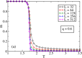
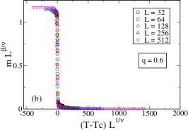
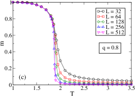
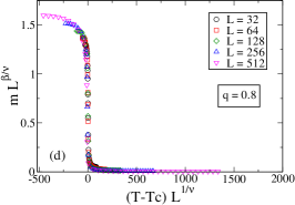
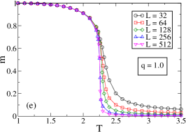
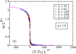
where $\langle\;\rangle$ stands for MC averages and $e$ is the energy per spin (we have considered $J=k=1$ for simplicity). In Fig. 1 it is shown the simulations in the range $0.5<q\leq 1.0$, where we present on the left side the magnetization versus the temperature for $q=0.6$, $q=0.8$, and $q=1.0$. As may be observed on this figure, the magnetization curves changes continuously from a ordered ferromagnetic phase to a disordered paramagnetic one. Thus, the critical exponents and the critical temperatures of the model can be obtained by the standard finite-size scaling (FSS) forms,

$$m(T,L) = L^{-\beta/\nu}\;\tilde{m}((T-T_{c})\;L^{1/\nu})~{},$$

$$\chi(T,L) = L^{\gamma/\nu}\;\tilde{\chi}((T-T_{c})\;L^{1/\nu})~{},$$

$$C(T,L) = L^{\alpha/\nu}\;\tilde{C}((T-T_{c})\;L^{1/\nu})~{},$$

$$T_{c}(L) = T_{c}+a\;L^{-1/\nu}~{},$$

Figure 2: (Color online) The pseudo-critical temperatures $T_{c}(L)$ versus $L^{-1}$ for some values of $q$. The extrapolation given us the critical temperatures $T_{c}$ in the thermodynamic limit ($L^{-1}\to 0$). Notice that for the $q\leq 0.5$ case the $T_{c}(L)$ values do not depend on $L$.

$q$	$T_{c}$	$\alpha$	$\beta$	$\gamma$	$\nu$
0.6	1.761 $\pm$ 0.003	0.34 $\pm$ 0.01	0.025 $\pm$ 0.001	1.69 $\pm$ 0.04	1.00 $\pm$ 0.01
0.8	1.891 $\pm$ 0.007	0.15 $\pm$ 0.02	0.075 $\pm$ 0.002	1.71 $\pm$ 0.04	1.00 $\pm$ 0.01
1.0	2.259 $\pm$ 0.011	0.00 $\pm$ 0.00	0.124 $\pm$ 0.006	1.75 $\pm$ 0.01	1.00 $\pm$ 0.02

Table 1: Three different entropic indexes in the range $0.5<q\leq 1.0$ and its respective critical temperatures and exponents $\alpha$, $\beta$, $\gamma$ and $\nu$. For $q=1$, the critical exponents and temperature are very close those expected, $\alpha=0.0$, $\beta=0.125$, $\nu=1.0$, $\gamma=1.75$ and $T_{c}=2.269$. Notice that the exponents $\nu$ are essentially the same for the three cases, whereas $\alpha$, $\beta$, $\gamma$ and $T_{c}$ depends on $q$. We have found a logarithmic dependence of $\alpha$ on the lattice size $L$ in the $q=1$ case, as expected, which give us $\alpha(q=1)=0$. The errors in the numerical estimates of the critical temperatures and the critical exponents are also presented.

Figure 3: (Color online) Upper figures: Binder cumulant, Eq.(11), versus temperature for $q=0.6$ [Fig. 3(a)] and the best collapse of data [Fig. 3(b)], based on the FSS in Eq.(12). The parameters are $\nu=1.0$ and $T_{c}=1.761$. Lower figures: magnetization values at each pseudo-critical temperature $T_{c}(L)$ for various lattice sizes $L$ [Fig. 3(c)] and the corresponding values of the susceptibility peaks [Fig. 3(d)], for $q=0.6$. The fittings in the log-log scale give us the corresponding values of the critical exponents ratios $\beta/\nu$ and $\gamma/\nu$, $0.025\pm 0.001$ and $1.69\pm 0.04$, respectively.

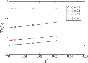
where $a$ is a constant. In Eqs. (III), the exponent $\beta$ is related to the behavior of the magnetization near the critical point $T_{c}$, $\nu$ is related to the divergence of the correlation length, $\gamma$ governs the divergence of the susceptibility at the critical point, $\alpha$ is related to the divergence of the specific heat at $T_{c}$ and $\tilde{m}$, $\tilde{\chi}$ and $\tilde{C}$ are scaling functions. The critical temperatures of the infinite lattices $T_{c}$ were obtained by extrapolating the $T_{c}(L)$ values given by the susceptibility peaks positions¹ (see Fig. 2). On the other hand, the exponents $\nu$ were obtained by means of the Binder cumulant binder , defined as

$$U_{L}=1-\frac{\langle\,m^{4}\rangle}{3\langle\,m^{2}\rangle^{2}}~{},$$ (11)

which has the FSS form

$$U_{L}=\tilde{U_{L}}((T-T_{c})\;L^{1/\nu})~{},$$ (12)

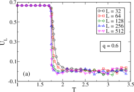
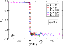
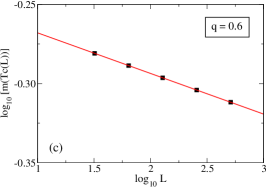
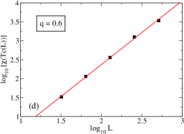
where $\tilde{U_{L}}$ is a scaling function that is independent of $L$. The error bars in the estimations of $\nu$ were obtained following the standard procedure for collapsing data of the Binder cumulant in the finite-size scaling approach, i.e., by monitoring small variations around the best collapsing pictures. In Fig.3 we show, as an example, the Binder cumulant for $q=0.6$ [Fig. 3(a)] and the best collapse of data [Fig. 3(b)], based on Eq.(12), obtained with the critical temperature $T_{c}$ and the exponent $\nu$ given in Table 1. Also in Fig.3 we show, for $q=0.6$, the values of the magnetization at the pseudo-critical points $T_{c}(L)$ for various lattice sizes $L$ [Fig. 3(c)] and the corresponding values of the susceptibility peaks positions [Fig. 3(d)], in the log-log scale. Linear fitting of data yield the parameters:

$$\beta/\nu = 0.025\pm 0.001~{},$$ (13)

$$\gamma/\nu = 1.69\pm 0.04~{}.$$ (14)

By repeating the fitting procedures of the specific heat peaks positions versus the lattice size $L$, in the log-log scale, we have estimated the ratio $\alpha/\nu=0.34\pm 0.01$, for $q=0.6$ (see Table 1). We have calculated the exponent $\nu$ by means of the Binder cumulant, as above-discussed, which allowed us to estimate the critical exponents $\alpha$, $\beta$ and $\gamma$. The procedure was the same for the other values of the entropic index $q$, and the best collapse of the magnetization data, presented on the right side of Fig. 1, supports the validity of the FSS forms in Eqs. (III) and the reliability of the numerical results for the critical exponents. The obtained numerical results are summarized on Table 1. Note that for $q=1$, the critical exponents $\alpha$, $\beta$, $\gamma$ and $\nu$ are quite close to the exact known values of the standard 2D Ising model, as expected. However, for different values of $q$ in this range, we have found different values of the exponents $\alpha$, $\beta$ and $\gamma$, as we can see in Table 1, whereas the values of $\nu$ are the same, within the determined uncertainty. These results will be discussed in with more details bellow.

Figure 4: (Color online) Results for the magnetic susceptibility $\chi$ for $L=128$ and typical cases of $q<0.5$ [$q=0.2$, (a)] and $q>0.5$ [$q=0.8$, (b)]. It is also shown the specific heat curves for the same values of $q$ [(c) and (d), respectively]. Although it is possible to observe a jump on the left figures, the histograms of the energy states visited during the MC simulation [Figs. 4(e) and 4(f)], at the corresponding critical temperatures, show only one-peak structures, indicating continuous phase transitions, even for the case $q<0.5$. We have defined the energy as the fraction of unhappy bonds in the system, $e=(E+2N)/(4N)$, where $E$ is the total energy given by Eq. (7) and $N$ is the total number of spins.

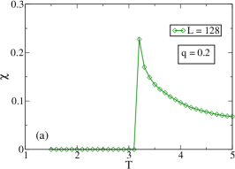
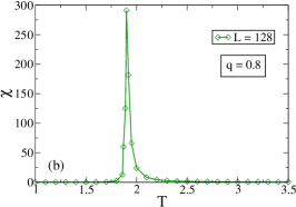
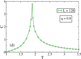
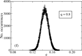
In Fig. 4 (right side) we show as example the susceptibility and the specific heat for $q=0.8$, as well as a histogram of the energy states visited during the dynamics of the system, at the critical temperature. This histogram shows only one peak, i.e., we have a continuous phase transition, as shown in the magnetization curves, Fig.1.

Figure 5: (Color online) Magnetization versus temperature for $q=0.2$ and $q=0.5$. We observe jumps on the curves at the corresponding critical points, but these $T_{c}$ values are independent of the lattice size, showing that the scaling naturally occurs on the $q\leq 0.5$ regime.

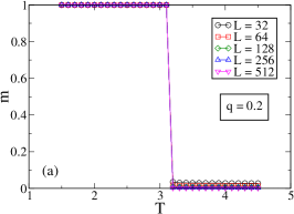
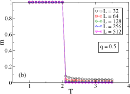
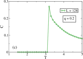
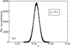
In Fig. 5 it is shown the behavior of the magnetization as a function of the temperature for two cases of $q\leq 0.5$. One can see that the critical temperatures, $T_{c}$ ², are the same for all lattice sizes, as shown in Fig. 2. This result is a consequence of the cutoff of the escort distribution, Eq.(3), and the magnetization jumps at $T_{c}$ from $m=1$ to $m=0$ (for more details, see 2008_EPJB_62_337 ). The cutoff also affects the susceptibility and the specific heat, as we can see in Figs. 4(a) and 4(c), respectively. However, if we compute histograms of the energy states visited during the dynamics³, at the critical temperatures, we can verify that we have only one peak for all $q\in[0,1]$, indicating the occurrence of continuous phase transitions [see Figs. 4(e) and (f)]. In other words, the cutoff keep the MC simulation trapped in the ground state for $T<T_{c}$ and the thermodynamic quantities suddenly change at $T_{c}$.

Figure 6: (Color online) The critical exponents $\alpha$, $\beta$ and $\gamma$ as functions of the entropic index $q$. In the range $0.5<q\leq 1.0$, the dependencies on $q$ are given by $\alpha(q)=(10\,q^{2}-33\,q+23)/20$, $\beta(q)=(2\,q-1)/8$ and $\gamma(q)=(q^{2}-q+7)/4$. The error bars for $\alpha$, $\beta$ and $\gamma$ fittings are less than 5%.

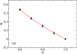
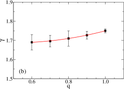
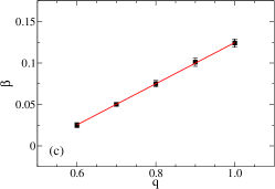
We can see from Table 1 that the critical exponent $\nu$ does not depends on $q$ in the range $0.5<q\leq 1.0$, and we conjecture that the correct value for any $q$ is $\nu=1.0$. However, $\alpha$, $\beta$ and $\gamma$ depend on the value of $q$. Fitting the numerical values of $\alpha$ with a second-order polynomial function of $q$, we have found that $\alpha(q)=0.5\,q^{2}-1.65\,q+1.15$, for $0.5<q\leq 1.0$ (see Fig. 6), or

$$\alpha(q)=\frac{1}{20}(10q^{2}-33q+23),$$ (15)

which give us the exact known value $\alpha(q=1)=0$ ⁴, and $\alpha(q=0.8)=0.15$ and $\alpha(q=0.6)=0.34$, in agreement with the values given in Tab. 1. In addition, fitting the numerical values of $\gamma$ also with a second-order polynomial function of $q$, we have found that $\gamma(q)=0.25\,q^{2}-0.25\,q+1.75$, for $0.5<q\leq 1.0$ (see Fig. 6), or

$$\gamma(q)=\frac{1}{4}(q^{2}-q+7),$$ (16)

which give us the exact known value $\gamma(q=1)=\frac{7}{4}$, $\gamma(q=0.8)=1.69$ and $\gamma(q=0.6)=1.71$. These results are also close to the ones obtained numerically. On the other hand, fitting the numerical values of $\beta$ with a straight line, we have found that $\beta(q)=-0.124+0.249\,q$, for $0.5<q\leq 1.0$ (see Fig. 6). We may conjecture that the exact dependence of $\beta$ on $q$ in this range is

$$\beta(q)=\frac{1}{8}(2q-1),$$ (17)

which give us the exact known value $\beta(q=1)=\frac{1}{8}$, $\beta(q=0.8)=0.075$ and $\beta(q=0.6)=0.025$, values that are also close to ones the obtained numerically.

These results suggest a nonuniversality of the critical exponents along the ferromagnetic-paramagnetic frontier. In addition, it also suggest that the scaling relations

$$2\,\beta+\gamma = d\,\nu~{},$$

$$\alpha+2\,\beta+\gamma = 2~{},$$ (18)

where $d$ is the dimension of the lattice ($d=2$ for the square lattice), should be changed. Thus, if we consider the above dependence of $\alpha$, $\beta$ and $\gamma$ on $q$, the first scaling relation of Eqs. (III), will become

$$2\,\beta+\gamma = (d+n_{q})\,\nu~{},$$ (19)

where

$$n_{q} = \frac{1}{4}\left(q^{2}+q-2\right)~{}.$$ (20)

Notice that for $q=1$, one has $n_{1}=0$, and the standard scaling relation is recovered. On the other hand, although $\alpha$, $\beta$, and $\gamma$ depend on the entropic index $q$, the Rushbrooke equality is satisfied for all $0.5<q\leq 1.0$, within uncertainty.

IV Conclusions

We have studied the Ising model with nearest-neighbors interactions on a square lattice by means of numerical Monte Carlo simulations. In our approach, different from other authors 1999_PhysA_268_553 ; 2000_PhysA_283_59 ; 1996_PhysA_233_395 ; 1997_PhysA_242_250 ; 1997_PhysA_247_553 , we simply changed the weight in the Metropolis algorithm to a ratio between the escort probabilities of the nonextensive statistics. This study was motivated by possible connection of the Tsallis statistics and some manganese oxides, called manganites, like $\mathrm{La_{0.60}Y_{0.07}Ca_{0.33}MnO_{3}}$ 2006_PRB_73_092401 ; 2002_PRB_66_134417 ; 2002_EPL_58_42 ; 2003_PRB_68_014404 . Due to computational cost, our simulations were done after $10^{7}$ Monte Carlo steps, with the entropic index $q\in[0,1]$ and the linear lattice sizes $L=32,64,128,256$ and $512$.

The Monte Carlo simulation of an Ising model with nearest-neighbors interactions showed a distinct behavior of the same system considered in the infinite-range-interaction limit 2003_PRB_68_014404 . Jumps on the magnetization and susceptibility curves in the range $0.0<q<0.5$ occur in both approaches, but for short-range interactions we do not have first-order phase transitions. In addition, the mean-field calculations foresee the same critical exponents of the 2D Ising model in the framework of the Boltzmann-Gibbs statistics. However, our calculation of the magnetization, the susceptibility and the specific heat for the short-range interacting system showed that three of the critical exponents depend on $q$ in the range $0.5<q\leq 1.0$.

Finite-size scaling analysis of the results showed that the critical exponents $\alpha$, $\beta$ and $\gamma$, that are related to the behavior of the specific heat, the magnetization and the susceptibility near the critical point $T_{c}$, respectively, depend on $q$ in the range $0.5<q\leq 1.0$. Based on the numerical estimates of these exponents, we conclude that the dependencies are of the form $\alpha(q)=(10\,q^{2}-33\,q+23)/20$, $\beta(q)=(2\,q-1)/8$ and $\gamma(q)=(q^{2}-q+7)/4$. Although the exponents $\alpha$, $\beta$ and $\gamma$ depend on $q$, as well as the critical temperatures $T_{c}$ 2008_EPJB_62_337 , the exponent $\nu$ does not; we found that $\nu=1.0$ $\forall$ $q$. These dependencies of the critical exponents on the entropic index suggest a nonuniversality of those exponents along the ferromagnetic-paramagnetic frontier. It also suggest a violation of the scaling relations $\alpha+2\,\beta+\gamma=2$ (Rushbrooke equality) and $2\,\beta+\gamma=d\,\nu$. However, when we take into account the $q-$dependence of the critical exponents showed in Table 1, we notice that the former scaling relation should be changed to $2\,\beta+\gamma=(d+n_{q})\,\nu$, where $n_{q}=\left(q^{2}+q-2\right)/4$ (note that for $q=1$, we obtain $n_{1}=0$), but the Rushbrooke equality is not altered. Thus, the inhomogeneities introduced in the system by the nonextensive statistics may be responsible for the $q-$dependence of the critical exponents $\alpha$, $\beta$ and $\gamma$, as well as the critical temperatures $T_{c}$.

On the other hand, we have a completely different scenario in the range $0.0<q\leq 0.5$. The cutoff of the Tsallis distribution keep the system in the ground state (with $m=1$) for $T<T_{c}=4(1-q)$, and at $T_{c}$ the magnetization jumps suddenly to zero, i.e., to a equiprobable state 2008_EPJB_62_337 . In the same way, the susceptibility and the specific heat curves also present jumps at $T_{c}$, due to the cutoff. Although the presence of these jumps, the histograms of the energy states visited during the dynamics, at the critical temperatures, show only one-peak structures, which is a indicative of the occurrence of continuous phase transitions.

Previous works on long- and short-range interactions 1D Ising models 1999_PRL_83_4233 ; 2000_EPJB_17_679 ; 2001_PhysA_290_159 predict that the magnetization scales differently for $q<1.0$ and $q=1.0$ regimes. Therefore, in this work we showed that the magnetization of the short-range 2D Ising model scales also differently in two regimes: for $0.5<q\leq 1.0$ the system scales as a 2D Ising model, but for $q\leq 0.5$ the magnetization and the critical temperature are independent of the lattice size due to the cutoff; thus, the scaling appears naturally on the system.

Also in a previous work 1999_PhysA_268_553 , it was shown that 2D Ising model with nearest-neighbors interactions does not undergo phase transitions, except for $q=1.0$. The main difference between their approach and ours is related to the definition of the temperature scale. In that work 1999_PhysA_268_553 , the authors have chosen $\beta$ as the parameter related to the temperature scale and, in this work, we have chosen $\beta_{q}^{\prime}$. The relation between these parameters is given in Eq.(4). The advantage of our approach over previous one, for the choice of the temperature scale, is that ours is supported by previous description of the magnetic properties, experimentally and theoretically investigated, of manganites 2006_PRB_73_092401 ; 2006_EPJB_50_99 ; 2002_PRB_66_134417 ; 2002_EPL_58_42 ; 2003_PRB_68_014404 . Thus, based on that, we believe that the 2D Ising model undergoes a phase transition even for $q\neq 1.0$, and the scaling relations should be changed as described above.

Extensions of this work to describe inhomogeneous magnetic systems, i.e., systems in which the exchange interaction changes along the sites of the lattice, as well as the study of the effects of uniform and random magnetic fields, within a nonextensive approach would be of great interest, because it can yield some clues to questions about the connection of such systems and the nonextensive statistics.

Acknowledgments

The authors acknowledge S.M.D. Queirós for his comments. We would like to thanks the Brazilian funding agencies CNPq, CAPES and the Brazilian Millennium Institute for Quantum Information for the financial supports. D.O.S.P. thanks FAPESP for financial support, M.S.R. thanks the financial support from PCI-CBPF program and A.M.S. would like to thanks the Ontario Goverment.

References

- (1) C. Tsallis, J. Stat. Phys. 52, 479 (1988).
- (2) C. Tsallis, Introduction to Nonextensive Statstical Mechanics: Approaching a Complex World. Springer, New York, 2009.
- (3) F. Baldovin and A. Robledo, Phys. Rev. E 66, 045104 (2002).
- (4) C. Tsallis, Physica A 340, 1 (2004).
- (5) S. M. D. Queirós, Europhys. Lett. 71, 339 (2005).
- (6) M. S. Reis, V. S. Amaral, R. S. Sarthour, and I. S. Oliveira, Phys. Rev. B 73, 092401 (2006).
- (7) M. S. Reis, V. S. Amaral, R. S. Sarthour and I. S. Oliveira, Eur. Phys. J. B 50, 99 (2006).
- (8) S. M. D. Queirós, Braz. J. Phys. 38, 203 (2008).
- (9) For a complete and updated list of references, see the web site: tsallis.cat.cbpf.br/biblio.htm.
- (10) C. Tsallis, M. Gell-Mann and Y. Sato, Proc. Natl. Acad. Sc. USA 102, 15377 (2005).
- (11) A. Rodríguez, V. Schwämmle and C. Tsallis, J. Stat. Mech. P09006 (2008).
- (12) F. Caruso and C. Tsallis, Phys. Rev. E 78, 021102 (2008).
- (13) F. P. Agostini, D. O. Soares-Pinto, M. A. Moret, C. Oshtoff and P. G. Pascutti, J. Comput. Chem. 27, 1142 (2006).
- (14) S. M. D. Queirós, L. G. Moyano, J. de Souza and C. Tsallis, Eur. Phys. J. B 55, 161 (2007).
- (15) B. M. Boghosian, Phys. Rev. E 53, 4754 (1996).
- (16) D. O. Soares-Pinto, M. S. Reis, R. S. Sarthour and I. S. Oliveira, J. Stat. Mech. P0807 (2007).
- (17) M. S. Reis, J. P. Araújo, V. S. Amaral, E. K. Lenzi and I. S. Oliveira, Phys. Rev. B 66, 134417 (2002).
- (18) M. S. Reis, J. C. C. Freitas, M. T. D. Orlando, E. K. Lenzi and I. S. Oliveira, Europhys. Lett. 58, 42 (2002).
- (19) M. S. Reis, V. S. Amaral, J. P. Araújo and I. S. Oliveira, Phys. Rev. B 68, 014404 (2003).
- (20) V. S. Amaral, J. P. Araújo, Y. P. Pogorelov, P. B. Tavares, J. B. Sousa and J. M. Vieira, J. Magn. Magn. Mater. 242, 655 (2002).
- (21) D. O. Soares-Pinto, I. S. Oliveira and M. S. Reis, Eur. Phys. J. B 62, 337 (2008).
- (22) C. Tsallis, R. S. Mendes and A. R. Plastino, Physica A 261, 534 (1998).
- (23) C. Tsallis, Nonextensive Entropy - Interdisciplinary Applications, chapter Nonextensive statistical mechanics: Construction and physical interpretation. eds. M. Gell-Mann and C. Tsallis. Oxford University Press, New York, 2004.
- (24) C. Beck and F. Schlogl, Thermodynamics of Chaotic Systems: An Introduction. Cambridge University Press, Cambridge, 1993.
- (25) A. R. Lima, J. S. S. Martins and T. J. P. Penna, Physica A 268, 553 (1999).
- (26) R. Salazar and R. Toral, Physica A 283, 59 (2000).
- (27) S. Martínez, F. Pennini and A.Plastino, Physica A 295, 246 (2001).
- (28) S. Martínez, F. Pennini and A. Plastino, Physica A 295, 416 (2001).
- (29) S. Abe, S. Martínez, F. Pennini and A. Plastino, Phys. Lett. A 281, 126 (2001).
- (30) R. Toral and R. Salazar, Physica A 305, 52 (2002).
- (31) R. Toral, Physica A 317, 209 (2003).
- (32) Q. A. Wang, L. Nivanen, A. LeMéhauté and M. Pezeril, Europhys. Lett. 65, 606 (2004).
- (33) S. Abe, Physica A 368, 430 (2006).
- (34) A. Linke, D. W. Heermann, P. Altevogt and M. Siegert, Physica A 222, 205 (1995).
- (35) D. Stauffer, Physica A 244, 344 (1997).
- (36) R. H. Landau and M. J. Paez, Computational Physics: Problem solving with computers. Wiley-VHC, Weinheim, 2004.
- (37) K. Binder, Z. Phys. B 43, 119 (1981).
- (38) C. Tsallis and D. A. Stariolo, Physica A 233, 395 (1996).
- (39) U. H. E. Hansmann, Physica A 242, 250 (1997).
- (40) I. Andricioaei and J. E. Straub, Physica A 247, 553 (1997).
- (41) R. Salazar and R. Toral, Phys. Rev. Lett. 83, 4233 (1999).
- (42) R. Salazar, A. R. Plastino and R. Toral, Eur. Phys. J. B 17, 679 (2000).
- (43) R. Salazar and R. Toral, Physica A 290, 159 (2001).