On the modification of the Efimov spectrum in a finite cubic box

Abstract

Three particles with large scattering length display a universal spectrum of three-body bound states called “Efimov trimers”. We calculate the modification of the Efimov trimers of three identical bosons in a finite cubic box and compute the dependence of their energies on the box size using effective field theory. Previous calculations for positive scattering length that were perturbative in the finite volume energy shift are extended to arbitrarily large shifts and negative scattering lengths. The renormalization of the effective field theory in the finite volume is explicitly verified. We investigate the effects of partial wave mixing and study the behavior of shallow trimers near the dimer energy. Moreover, we provide numerical evidence for universal scaling of the finite volume corrections.

I Introduction

Few-body systems with resonant interactions characterized by a large scattering length $a$ show interesting universal properties. If $a$ is positive, two particles of mass $m$ form a shallow dimer with energy $E_{2}\approx-{\hbar^{2}}/{(ma^{2})}\,$, independent of the mechanism responsible for the large scattering length. Examples for such shallow dimer states are the deuteron in nuclear physics, the ⁴He dimer in atomic physics, and possibly the new charmonium state $X(3872)$ in particle physics Braaten:2004rn ; Platter:2009gz . In the three-body system, the universal properties include the Efimov effect Efimov-70 . If at least two of the three pairs of particles have a large scattering length $|a|$ compared to the range $r_{0}$ of their interaction, there is a sequence of three-body bound states whose energies are spaced geometrically between $-\hbar^{2}/mr_{0}^{2}$ and $-\hbar^{2}/ma^{2}$. In the limit $1/a\to 0$, there are infinitely many bound states with an accumulation point at the three-body scattering threshold. These Efimov states or trimers have a geometric spectrum Efimov-70 :

$$E^{(n)}_{3}=-(e^{-2\pi/s_{0}})^{n-n_{*}}\hbar^{2}\kappa^{2}_{*}/m,$$ (1)

which is specified by the binding momentum $\kappa_{*}$ of the Efimov trimer labeled by $n_{*}$. This spectrum is a consequence of a discrete scaling symmetry with discrete scaling factor $e^{\pi/s_{0}}$. In the case of identical bosons, $s_{0}\approx 1.00624$ and the discrete scaling factor is $e^{\pi/s_{0}}\approx 22.7$. The discrete scale invariance persists if $a$ is large but finite, but in this case it connects states corresponding to different values of the scattering length. The scaling symmetry becomes also manifest in the log-periodic dependence of scattering observables on the scattering length $a$ Efimov79 . The consequences of discrete scale invariance and “Efimov physics” can be calculated in an effective field theory for short-range interactions, where the Efimov effect appears as a consequence of a renormalization group limit cycle Bedaque:1998kg .

While the Efimov effect was established theoretically already in 1970, first experimental evidence for an Efimov trimer in ultracold Cs atoms was provided only recently by its signature in the three-body recombination rate Kraemer-06 . It could be unravelled by varying the scattering length $a$ over several orders of magnitude using a Feshbach resonance. Since this pioneering experiment, there was significant experimental progress in observing Efimov physics in ultracold quantum gases. More recently, evidence for Efimov trimers was also obtained in atom-dimer scattering Knoop08 and in three-body recombination in a balanced mixture of atoms in three different hyperfine states of ⁶Li Ottenstein08 ; Huckans08 , in a mixture of Potassium and Rubidium atoms Barontini09 , and in an ultracold gas of ⁷Li atoms Gross09 . In another experiment with Potassium atoms Zaccanti09 , two bound trimers were observed.

The observation of Efimov physics in nuclear and particle physics systems is complicated by the inability to vary the scattering length and one has to focus on the detection of excited states. While two-neutron halo nuclei could be bound due to the Efimov effect, the analysis of known halo nuclei does not show much promise for an unambiguous identification (See Ref. Canham:2008jd and references therein). Another opportunity to observe Efimov physics is given by lattice QCD simulations of three-nucleon systems Wilson:2004de . A number of studies of the quark-mass dependence of the chiral nucleon-nucleon ($NN$) interaction found that the inverse scattering lengths in the relevant ${}^{3}{\rm S}_{1}$–${}^{3}{\rm D}_{1}$ and ${}^{1}{\rm S}_{0}$ channels may both vanish if one extrapolates away from the physical values to slightly larger quark masses Beane:2001bc ; Beane:2002xf ; Epelbaum:2002gb . This implies that QCD is close to the critical trajectory for an infrared renormalization group limit cycle in the three-nucleon sector. It was conjectured that QCD could be tuned to lie precisely on the critical trajectory by tuning the up and down quark masses separately Braaten:2003eu . As a consequence, the triton would display the Efimov effect. More refined studies of the signature of Efimov physics in this case followed Epelbaum:2006jc ; Hammer:2007kq . However, a proof of this conjecture can only be given by an observation of this effect in a lattice QCD simulation Wilson:2004de . The first full lattice QCD calculation of nucleon-nucleon scattering was reported in Beane:2006mx but statistical noise presented a serious challenge. A promising recent high-statistics study of three-baryon systems presented also initial results for a system with the quantum numbers of the triton such that lattice QCD calculations of three-nucleon systems are now within sight Beane:2009gs . For a review of these activities, see Ref. Beane:2008dv . Since lattice simulations are carried out in a cubic box, it is important to understand the properties of Efimov states in the box. The first step towards this goal is to understand these modifications for a system of three identical bosons.

The corresponding modifications of the Efimov spectrum can be calculated in effective field theory (EFT) since the finite volume modifies the infrared properties of the system. The properties of two-body systems with large scattering length in a cubic box were calculated in Ref. Beane:2003da . Some properties of three-body systems in a finite volume have also been studied previously. For repulsive and weakly attractive interactions without bound states, Tan has determined the volume dependence of the ground state energy of three bosons up to $\mathcal{O}((a/L)^{7})$ Tan08 . In Refs. Beane:2007qr ; Detmold:2008gh , this result was extended for general systems of $N$ bosons. It was used to analyze recent results for three and more boson systems from lattice QCD Beane:2007es ; Detmold:2008fn ; Detmold:2008yn . For the unitary limit of infinite scattering length, some studies have been carried out as well. The properties of three spin-1/2 fermions in a box were investigated in Pricoup07 . However, this system has no three-body bound states in the infinite volume. The volume dependence of energy levels in a finite volume can also be used to extract scattering phase shifts and resonance properties from lattice calculations Luscher:1990ux ; Luscher:1991cf . For a recent application of this idea to the $\Delta(1232)$ resonance, see Refs. UGM1 ; UGM2 .

In a previous letter, we have investigated the finite volume corrections for a three-boson system with large but finite scattering length Kreuzer:2008bi . We have studied the modification of the bound state spectrum for positive scattering length using an expansion valid for small finite volume shifts and explicitly verified the renormalization in the finite box within this approximation. In the current paper, we present an extension of this work that avoids the expansion in the energy shift and can be applied to arbitrarily large shifts. Moreover, we extend our previous studies to the case of negative scattering lengths. Our results indicate that the finite volume corrections are subject to a universal scaling relation. We also provide a more detailed discussion of the technical details and our numerical method.

II Theoretical Framework

II.1 Lagrangian and Boson-Diboson Amplitude

Three identical bosons interacting via short-range forces can be described by the Lagrangian Bedaque:1998kg ; Braaten:2004rn

$$\mathcal{L}=\psi^{\dagger}\left(i\partial_{t}+\frac{1}{2}\nabla^{2}\right)\psi+\frac{g_{2}}{4}d^{\dagger}d-\frac{g_{2}}{4}\left(d^{\dagger}\psi^{2}+\mathrm{h.c.}\right)-\frac{g_{3}}{36}d^{\dagger}d\psi^{\dagger}\psi+\ldots\,,$$ (2)

where the dots indicate higher order terms. The degrees of freedom in the Lagrangian are a boson field $\psi$ and a non-dynamical auxiliary field $d$ representing the composite of two bosons. Units have been chosen such that $\hbar=m=1$. This Lagrangian corresponds to the zero range limit with $r_{0}=0$. Our results will therefore be applicable to physical states whose size is large compared to $r_{0}$. Corrections from finite range can be included via higher order terms in the Lagrangian but will not be considered here. The coupling constants $g_{2}$ and $g_{3}$ will be determined by matching calculated observables to a two-body datum and a three-body datum, respectively. The central quantity in the three-body sector of this EFT is the boson-diboson scattering amplitude. It determines all three-body observables and is given as the solution of an inhomogeneous integral equation, depicted diagrammatically in Fig. 1. A detailed discussion of the infinite volume case can be found in Braaten:2004rn . Here we follow the strategy of Refs. Kreuzer:2008bi ; Beane:2003da and focus on the finite volume case.

Figure 1: Integral/sum equation for the boson-diboson amplitude. The narrow lines denote the boson propagator and the thick lines denote the full diboson propagator.

The system of three bosons is assumed to be contained in a cubic box with side length $L$ and periodic boundary conditions. This leads to quantized momenta $\vec{k}=\frac{2\pi}{L}\vec{n},\,\vec{n}\in\mathbb{Z}^{3}$. In particular, the possible loop momenta are quantized. As a consequence, the integration over loop momenta is replaced by an infinite sum. The divergent loop sums are regulated by a momentum cutoff $\Lambda$ similar to the infinite volume case.

The finite volume modifies the infrared physics of the system but does not change the ultraviolet behavior of the amplitudes. Therefore, the renormalization is the same in the infinite and finite volume cases. Of course, this statement only holds if the momentum cutoff $\Lambda$ is large compared to the momentum scale set by the size of the volume, namely $2\pi/L$, such that the infrared and the ultraviolet regime are well separated. In the numerical calculations presented in this work, the consistent renormalization of the results will always be verified explicitly. The two-body sector can be completely renormalized by matching the two-body coupling constant $g_{2}$ to a low-energy two-body observable, namely the two-body scattering length $a$ or the dimer binding energy. Because of the discrete scaling symmetry, the three-body coupling approaches an ultraviolet limit cycle. For convenience, the three-body coupling constant $g_{3}$ is expressed in the form $g_{3}=-9g_{2}^{2}H(\Lambda)/\Lambda^{2}$. The cutoff dependence of the dimensionless function $H(\Lambda)$ is then given by Braaten:2004rn

$$H(\Lambda)=\frac{\cos\left[s_{0}\log(\Lambda/\Lambda_{\ast})+\arctan s_{0}\right]}{\cos\left[s_{0}\log(\Lambda/\Lambda_{\ast})-\arctan s_{0}\right]},$$ (3)

where $s_{0}\approx 1.00624\dots$ and $\Lambda_{\ast}\approx 2.62\kappa_{*}$ is a three-body parameter that can be fixed from a trimer binding energy or another three-body datum.

Figure 2: The full diboson propagator (thick solid line) is obtained by dressing the bare diboson propagator (double lines) with bosonic loops (narrow solid lines).

For the diboson lines in the three-body equation depicted in Fig. 1, the full, interacting diboson propagator $D$ has to be used. This quantity corresponds to the exact two-body scattering amplitude. It is obtained by dressing the bare diboson propagator, given by the constant $4i/g_{2}$, with bosonic loops as shown in Fig. 2. This leads to an infinite sum that can be evaluated analytically. For a diboson with energy $E$, the propagator is

$$D(E)=\frac{32\pi}{g_{2}^{2}}\Bigg{[}\frac{1}{a}-\sqrt{-E}+\frac{1}{L}\sum_{\begin{subarray}{c}\vec{\jmath}\in\mathbb{Z}^{3}\\ \vec{\jmath}\neq 0\end{subarray}}\frac{1}{|\vec{\jmath}|}\mathrm{e}^{-|\vec{\jmath}|L\sqrt{-E}}\Bigg{]}^{-1}\,.$$ (4)

In the limit $L\to\infty$, this expression reduces to the full diboson propagator in the infinite volume case.

Having obtained the full diboson propagator, the integral equation for the boson-diboson scattering amplitude can be written down explicitly. Using the diagrammatical representation in Fig. 1 and the Feynman rules derived from the effective Lagrangian (2), we obtain:

$$\mathcal{A}(\vec{p},\vec{k};E) = -\frac{g_{2}^{2}}{4}\frac{1}{E-p^{2}/2-k^{2}/2-(\vec{p}+\vec{k})^{2}/2}-\frac{g_{3}}{36}$$

$$\quad+i\int\frac{\mathrm{d}{q_{0}}}{(2\pi)}\,L^{-3}\sum_{\vec{q}\in\frac{2\pi}{L}\mathbb{Z}^{3}}\left[\frac{g_{2}^{2}}{4}\;\frac{1}{q_{0}-q^{2}/2}\;\frac{D(E-q_{0}+q^{2}/4)}{E-p^{2}/2-q_{0}-(\vec{p}+\vec{q})^{2}/2}\right.$$

$$\hskip 128.0374pt\left.+\frac{g_{3}}{36}\frac{1}{q_{0}-q^{2}/2}D(E-q_{0}+q^{2}/4)\right]\mathcal{A}(\vec{q},\vec{k};E)$$

Here, $\vec{p}$ ($\vec{k}$) are the momenta of the incoming (outgoing) dibosons, while the momenta of the incoming (outgoing) bosons are $-\vec{p}$ ($-\vec{k}$). The boson legs have been put on shell but the diboson legs remain off-shell. The total energy of the system, $E$, can be treated as a parameter of the equation. The integration over the loop energy can be performed by virtue of the residue theorem. This yields the sum equation

$$\mathcal{A}(\vec{p},\vec{k};E)=-\frac{g_{2}^{2}}{4}\mathcal{Z}_{E}(\vec{p},\vec{k})+\frac{8\pi}{L^{3}}\sum_{\vec{q}\in\frac{2\pi}{L}\mathbb{Z}^{3}}\mathcal{Z}_{E}(\vec{p},\vec{q})\tau_{E}(q)\mathcal{A}(\vec{q},\vec{k};E),$$ (6)

with

$$\mathcal{Z}_{E}(\vec{p},\vec{k}) =\left[\left(p^{2}+\vec{p}\cdot\vec{k}+k^{2}-E\right)^{-1}+\frac{H(\Lambda)}{\Lambda^{2}}\right],$$ (7)

$$\tau_{E}(q) =\bigg{[}\frac{1}{a}-\sqrt{\frac{3q^{2}}{4}-E}+\sum_{\begin{subarray}{c}\vec{\jmath}\in\mathbb{Z}^{3}\\ \vec{\jmath}\neq 0\end{subarray}}\frac{1}{L|\vec{\jmath}|}\mathrm{e}^{-|\vec{\jmath}|L\sqrt{\frac{3q^{2}}{4}-E}}\bigg{]}^{-1}.$$ (8)

If the energy $E$ is near a trimer energy $E_{3}^{(n)}<0$, the amplitude $\mathcal{A}$ exhibits a simple pole and the dependence on the momenta seperates:

$$\mathcal{A}(\vec{p},\vec{k};E)\longrightarrow\frac{\mathcal{F}(\vec{p})\mathcal{F}(\vec{k})}{E-E_{3}^{(n)}},\quad\mbox{as }E\rightarrow E_{3}^{(n)}.$$ (9)

Matching the residues on both sides of Eq. (6), the bound-state equation

$$\mathcal{F}(\vec{p})=\frac{8\pi}{L^{3}}\sum_{\vec{q}\in\frac{2\pi}{L}\mathbb{Z}^{3}}\mathcal{Z}_{E}(\vec{p},\vec{q})\tau_{E}(q)\mathcal{F}(\vec{q})$$ (10)

is obtained. Values of the energy $E$, for which this homogeneous sum equation has a solution, are identified with the energies $E_{3}^{(n)}$ of the trimer states.

II.2 Cubic symmetry

In the infinite volume case, only s-wave bound states are formed. However, in a finite cubic volume, the spherical symmetry of the infinite volume is broken to a cubic symmetry. In the language of group theory, the infinitely many irreducible representations of the spherical symmetry group $O(3)$ are mapped onto the five irreducible representations of the cubic group $O$. The representations of the spherical symmetry group are now reducible and can therefore be decomposed in terms of the five irreducible representations of the cubic group. On the other hand, a quantity $\psi_{s}$ transforming according to the irreducible representation $s$ of $O$ can be written in terms of the basis functions of the spherical symmetry, i.e. the spherical harmonics $Y_{lm}$, via

$$\psi_{s}(\vec{r})=\sum_{\ell,t}R_{\ell t}(r)K_{s\ell t}(\hat{r})=\sum_{\ell,t}R_{\ell t}(r)\left[\sum_{m}C_{s\ell m}^{(t)}Y_{\ell m}(\hat{r})\right],$$ (11)

where $\hat{r}=\vec{r}/|\vec{r}|$ and $t$ is an additional index needed if the representation labeled by $\ell$ appears in the irreducible representation $s$ more than once. The linear combinations $K_{s\ell t}$ of spherical harmonics are called “kubic harmonics” BetheVdLage:47 . The values of the coefficients $C_{s\ell m}^{(t)}$ are known for values of $\ell$ as large as 12 Altmann:65 .

In order to make contact with the infinite volume formalism, Eq. (10) is rewritten using Poisson’s resummation formula. This identity states that an infinite sum over integer vectors may be replaced by an infinite sum over integer vectors of the Fourier transform of the addend, i.e.

$$\sum_{\vec{n}\in\mathbb{Z}^{3}}f(\vec{n})=\sum_{\vec{m}\in\mathbb{Z}^{3}}\hat{f}(\vec{m})$$ (12)

where $\hat{f}(\vec{m})=\int_{\mathbb{R}^{3}}\mathrm{d}^{3}{y}\,\mathrm{e}^{\mathrm{i}2\pi\vec{m}\cdot\vec{y}}f(\vec{y})$ is the Fourier transform of $f$. Applying the identity (12) to Eq. (10) yields

$$\mathcal{F}(\vec{p})=\frac{1}{\pi^{2}}\sum_{\vec{n}\in\mathbb{Z}^{3}}\int\mathrm{d}^{3}{y}\,\mathrm{e}^{\mathrm{i}L\vec{n}\cdot\vec{y}}\mathcal{Z}_{E}(\vec{p},\vec{y})\tau_{E}(y)\mathcal{F}(\vec{y}).$$ (13)

The term with $\vec{n}=\vec{0}$ gives the corresponding equation in the infinite volume, while the other terms of the infinite sum may be viewed as corrections due to momentum quantization and the breakdown of the spherical symmetry. The explicit recovery of the infinite volume term is useful for bound states, since in this case the analytic structure of the amplitude, i.e. the pole at the binding energy, is identical and only the position of the pole is changed. This approach may be inappropriate for states belonging to the continuous scattering region of the infinite volume.

In order to evaluate the angular integration in Eq. (13), all quantities with angular dependence are expanded in terms of the basis functions of the irreducible representations of $O(3)$, namely in spherical harmonics. The amplitude $\mathcal{F}$ itself is assumed to transform under the trivial representation $A_{1}$ of the cubic group, since the $\ell=0$ representation is solely contained in $A_{1}$. The amplitude can therefore be written as

$$\mathcal{F}(\vec{p})=\sum_{\ell,t}F_{\ell t}(p)K_{A_{1}\ell t}(\hat{p})=\sum^{(A_{1})}_{\ell,t}F_{\ell t}(p)\sum_{m=-\ell}^{\ell}C_{A_{1}\ell m}^{(t)}Y_{\ell m}(\hat{p}).$$ (14)

The sum runs over those values of $\ell$ associated with the $A_{1}$-representation of $O$. The first few values are $\ell=0,4,6,8,\dots$. Since the first occasion where an $\ell$-value appears more than once is $\ell=12$, the summation over the multiplicity and hence the index $t$ will be suppressed in the following.

The only angular dependence of the quantity $\mathcal{Z}_{E}(\vec{p},\vec{y})$ is on the cosine of the angle $\theta_{\vec{p}\vec{y}}$ between $\vec{p}$ and $\vec{y}$. Therefore, $\mathcal{Z}_{E}(\vec{p},\vec{y})$ can be expanded in Legendre polynomials $P_{\ell}(\cos\theta_{\vec{p}\vec{y}})$. These polynomials can in turn be expressed in spherical harmonics via the addition theorem, yielding

$$\mathcal{Z}_{E}(\vec{p},\vec{y})=\sum_{\ell=0}^{\infty}Z^{(\ell)}_{E}(p,y)P_{\ell}(\cos\theta_{\vec{p}\vec{y}})=\sum_{\ell=0}^{\infty}Z^{(\ell)}_{E}(p,y)\frac{4\pi}{2\ell+1}\sum_{m=-\ell}^{\ell}Y_{\ell m}^{\ast}(\hat{p})Y_{\ell m}(\hat{y}).$$ (15)

The exponential function in Eq. (13) can be rewritten using the identity

$$\mathrm{e}^{\mathrm{i}L\vec{n}\cdot\vec{y}}=4\pi\sum_{\ell=0}^{\infty}\mathrm{i}^{\ell}j_{\ell}(L|\vec{n}|y)\sum_{m=-\ell}^{\ell}Y_{\ell m}^{\ast}(\hat{n})Y_{\ell m}(\hat{y}),$$ (16)

where $j_{\ell}$ is the spherical Bessel function of order $\ell$.

With these expansions, the angular integration in Eq. (13) can be performed. The integral over the three spherical harmonics depending on $\hat{y}$ yields Wigner 3-$j$ symbols. Projecting on the $\ell$th partial wave results in an infinite set of coupled integral equations for the quantities $F_{\ell}$:

$$\begin{split}F_{\ell}(p)&=\frac{4}{\pi}\int_{0}^{\Lambda}\mathrm{d}y\,y^{2}\bigg{[}Z^{(\ell)}_{E}(p,y)\tau_{E}(y)\frac{1}{2\ell+1}F_{\ell}(y)\\ &\qquad\qquad+2\sqrt{\pi}\sum_{\begin{subarray}{c}\vec{n}\in\mathbb{Z}^{3}\\ \vec{n}\neq 0\end{subarray}}\sum_{{\ell^{\prime}},{m^{\prime}}}^{(A_{1})}\sum_{{\ell^{\prime\prime}},{m^{\prime\prime}}}\begin{pmatrix}{\ell^{\prime}}&{\ell^{\prime\prime}}&\ell\\ 0&0&0\end{pmatrix}\begin{pmatrix}{\ell^{\prime}}&{\ell^{\prime\prime}}&\ell\\ {m^{\prime}}&{m^{\prime\prime}}&0\end{pmatrix}\frac{C_{{\ell^{\prime}}{m^{\prime}}}}{C_{\ell 0}}Y_{{\ell^{\prime\prime}}{m^{\prime\prime}}}(\hat{n})\\ &\qquad\qquad\qquad\;\times\sqrt{\frac{(2{\ell^{\prime}}+1)(2{\ell^{\prime\prime}}+1)}{2\ell+1}}\;\mathrm{i}^{\ell^{\prime\prime}}j_{\ell^{\prime\prime}}(L|\vec{n}|y)Z^{(\ell)}_{E}(p,y)\tau_{E}(y)F_{{\ell^{\prime}}}(y)\bigg{]}.\end{split}$$ (17)

The ${\ell^{\prime}}$ sum runs over the partial waves associated with the $A_{1}$ representation. The quantity $Z^{(\ell)}_{E}(p,y)$ can be calculated from Eq. (15) to be

$$Z^{(\ell)}_{E}(p,y)=(2\ell+1)\left[\frac{1}{py}\,Q_{\ell}\left(\frac{p^{2}+y^{2}-E}{py}\right)+\frac{H(\Lambda)}{\Lambda^{2}}\delta_{\ell 0}\right].$$ (18)

Here, $Q_{\ell}$ is a Legendre function of the second kind. The three-body contact interaction contributes only to the s-wave, as expected.

Since the bound states in the infinite volume are s-wave states, Eq. (17) is specialized to the case $\ell=0$, yielding

$$\begin{split}F_{0}(p)=&\frac{4}{\pi}\int_{0}^{\Lambda}\mathrm{d}y\,y^{2}\bigg{[}Z_{E}^{(0)}(p,y)\tau_{E}(y)\bigg{(}1+\sum_{\begin{subarray}{c}\vec{n}\in\mathbb{Z}^{3}\\ \vec{n}\neq 0\end{subarray}}\frac{\sin(L|\vec{n}|y)}{L|\vec{n}|y}\bigg{)}F_{0}(y)\\ &+2\sqrt{\pi}\sum_{\begin{subarray}{c}\vec{n}\in\mathbb{Z}^{3}\\ \vec{n}\neq 0\end{subarray}}\sum_{{\ell^{\prime}}=4,6,\dots}^{(A_{1})}\sum_{{m^{\prime}}=-{\ell^{\prime}}}^{{\ell^{\prime}}}\mathrm{i}^{\ell^{\prime}}j_{\ell^{\prime}}(L|\vec{n}|y)Y_{{\ell^{\prime}}{m^{\prime}}}^{\ast}(\hat{n})Z_{E}^{(0)}(p,y)\tau_{E}(y)C_{{\ell^{\prime}}{m^{\prime}}}F_{\ell^{\prime}}(y)\bigg{]}\end{split}$$ (19)

The specialization of Eq. (18) to the case $\ell=0$ reads

$$Z_{E}^{(0)}(p,y)=\frac{1}{2py}\log\left(\frac{p^{2}+py+y^{2}-E}{p^{2}-py+y^{2}-E}\right)+\frac{H(\Lambda)}{\Lambda^{2}}.$$ (20)

	$\sum_{\begin{subarray}{c}\vec{n}\in\mathbb{Z}^{3}\\ |\vec{n}|=n\end{subarray}}\frac{1}{2}\left(Y_{\ell m}+Y_{\ell,-m}\right)$
$n$	$\ell=0,m=0$	$\ell=4,m=0$	$\ell=4,m=4$
101	606	96.23	81.33
1001	9126	$-$94.05	20.69
3501	39678	118.67	$-$15.73

Table 1: Integer vector sums over real combinations of $Y_{\ell m}$ for a given absolute value $n$ (“angular sums”). For higher partial waves, the value of the sum is smaller and the contribution of the partial wave is suppressed.

The second line of Eq. (19) indicates admixtures from higher partial waves. Since the leading term in the expansion of the spherical Bessel function is $1/(L|\vec{n}|y)$, these contributions are suppressed by at least $a/L$. They will therefore be small for volumes not too small compared to the size of the bound state. Moreover, contributions from higher partial waves will be suppressed kinematically for shallow states with small binding momentum. This is ensured by the spherical harmonic in the second line of Eq. (19). For higher partial waves, the angular sum yields smaller prefactors relative to the s-wave ($\ell=0$) for a given absolute value $n$ (see Table 1). Only for small lattices, i.e. when $a/L$ is large, this behavior is counteracted by terms stemming from the spherical Bessel function and higher partial waves may contribute significantly. The first numerical calculations presented in this work were therefore mainly performed neglecting contributions from higher partial waves. For two specific examples, however, we explicitly calculate the contribution from the next partial wave $\ell=4$ and demonstrate that it is small. Some details on the numerical solution of Eq. (19) are given in the Appendix. In the following section, we present our results.

III Results and discussion

By employing the formalism laid out in the previous section, we have calculated energy levels in finite cubic volumes of varying side lengths. The results of these calculations are presented in the following. For convenience, the dependence of the energies on the boson mass $m$ is reinstated in this section.

III.1 Positive scattering length

We first present results for systems with $a>0$. In this regime, a physical diboson state with a binding energy $E_{D}=-1/(ma^{2})$ exists. This energy is therefore identical with the threshold for the break-up of a trimer into a diboson and a single boson. We choose states with different energies in the infinite volume, including shallow as well as deeply bound states:

• $E_{3}^{\infty}\,=-1.18907/(ma^{2})$,  $\Lambda_{\ast}a=5.66$,

• $E_{3}^{\infty}\,=-27.4427/(ma^{2})$,  $\Lambda_{\ast}a=5.66$,

• $E_{3}^{\infty}\,=-9440.91/(ma^{2})$,  $\Lambda_{\ast}a=5.66$,

• $E_{3}^{\infty}\,=-5.04626/(ma^{2})$,  $\Lambda_{\ast}a=1.66$,

• $E_{3}^{\infty}\,=-11.1322/(ma^{2})$,  $\Lambda_{\ast}a=3.66$,

Here, $E_{3}^{\infty}$ is the trimer energy in the infinite volume. Note that the states Ia, Ib and Ic appear in the same physical system chracterized by $\Lambda_{\ast}a=5.66$. For each of these states, its energy in the finite cubic volume has been calculated for various values of the box side length $L$. In order to check the consistency of our results, the calculation was carried out for several cutoff momenta $\Lambda$. For each cutoff, the three-body interaction parameterized by $H(\Lambda)$ has been adjusted such that the infinite volume binding energies are identical for all considered values of $\Lambda$. If our results are properly renormalized, the results for the different cutoffs should agree with each other up to an uncertainty of order $1/(\Lambda a)$ stemming from the finiteness of the cutoff.

    

Figure 3: Variation of the trimer energy $E_{3}$ with the side length $L$ of the cubic volume for the states II (left) and III (right). Plotted are three datasets for different values of the cutoff parameter $\Lambda$, together with the $1/(\Lambda a)$ bands. The point $a/L=0$ corresponds to the infinite volume limit.

The results for the states II and III are depicted in Fig. 3 for box sizes between $L=6a$ and $L=a/2$. The values obtained for different cutoffs indeed agree with each other within the depicted uncertainty bands. Note that these bands do not represent corrections from higher orders of the EFT. For both states, the infinite volume limit is smoothly approached. As the volume becomes smaller, the energy of the states is more and more diminished. This corresponds to an increased binding with decreasing box size.

In the infinite volume, state III is more deeply bound than state II. Naïvely, one therefore expects the former to have a smaller spatial extent than the latter. The size of the state can be estimated via the formula $(-mE_{3}^{\infty})^{-1/2}$, yielding $0.45a$ for state II and $0.3a$ for state III. Hence, a given finite volume should affect state II more strongly than the smaller state III. This behavior can indeed be observed. For example, considering a cubic volume with side length $L=2a$, the energy of state II deviates 10% from the infinite volume value, whereas the corresponding difference for state III is less than one percent. On the other hand, the box size for which the energy shift of the state III amounts to 10% is roughly $1.3a$.

For both states, we can now form the dimensionless number $r=-mE_{3}^{\infty}L_{10\%}^{2}$, where $L_{10\%}$ is the box size at which the energy differs by 10% from the infinite volume value. This yields $r\approx 20$ for state II and $r\approx 19$ for state III. The approximate equality of the two values of $r$ may indicate the presence of universal scaling in the finite volume version of the Effective Theory.

Figure 4: Variation of the trimer energy $E_{3}$ with the side length $L$ of the cubic volume for state II. Plotted are three datasets for different values of the cutoff parameter $\Lambda$, together with the $1/(\Lambda a)$ bands, and one dataset obtained using a Taylor expanded version of the integral kernel.

In Fig. 4, the three datasets obtained for state II are plotted again, this time in comparison to the results from a calculation using the expansion of the kernel used in Ref. Kreuzer:2008bi and described in Appendix A. For large values of the box size $L$, the results of both calculations agree with each other. For volumes smaller than $1.7a$, the result of the calculation with the expansion deviates from the result of the full calculation. For this size of the volume, the full result differs by about 20% from the infinite volume binding energy. Accordingly, the expansion employed for the integral kernel can not be applicable any longer. In Fig. 4, results are only depicted for volumes with $L\geq a$. For smaller volumes, the results of calculations using the expansion become cutoff dependent, and are hence not are not properly renormalized anymore.

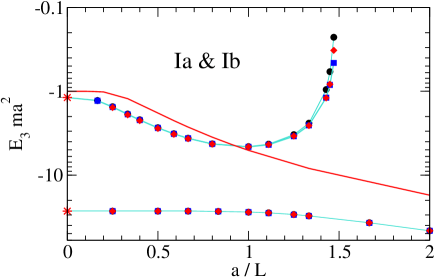
Figure 5: Variation of the trimer energy $E_{3}$ with the side length $L$ of the cubic volume for the states Ia (upper curve) and Ib (lower curve). Plotted are three datasets for different values of the cutoff parameter $\Lambda$, together with the $1/(\Lambda a)$ bands (circles: $\Lambda=200\,a^{-1}$; squares: $\Lambda=300\,a^{-1}$; diamonds: $\Lambda=400\,a^{-1}$). The solid line depicts the diboson energy.

In Fig. 5, we show our results for the two states Ia and Ib in the same physical system characterized by $\Lambda_{\ast}a=5.66$. The volume dependence of the two states is again shown for box sizes between $L=6a$ and $L=a/2$. The curve corresponding to the more deeply bound state Ib shows a behavior similar to the one observed for the states II and III. The binding energy remains constant until the volume is small enough to affect the state. At this point, the energy of the state is more and more diminished as the volume becomes smaller.

The behavior of the shallow state Ia is different. In the region $L\approx a$, the binding is not further increased. The results for smaller volumes show a sharp rise of the three-body energy. The energy of the state becomes positive near $L=0.67a$. State Ia is close to the threshold for boson-diboson scattering in the infinite volume located at $E_{D}=-1/(ma^{2})$. For comparison, we calculated the energy of the physical diboson according to Beane:2003da . The resulting curve is the solid line in Fig. 5. Like the energy of the three-body bound states, the energy of the diboson is diminished in finite volumes. For volumes of the size $L\approx 1.2a$, the energy of the three-body state Ia becomes larger than the diboson energy and starts to grow. This behavior is consistent with the observation that states are always shifted away from the threshold in a finite volume. In the two-body sector, for example, continuum states have been shown to have a power law dependence on the volume, while the volume dependence of bound states is dominated by exponentials Beane:2003da . The data shown for state Ia can be explained by an exponential for $L>a$, which characterizes the state as a bound state. For $L<a$, the data is consistent with a power law, indicating the state indeed behaves like a boson-diboson scattering state if its energy is above the diboson energy.

The other investigated states do not show such a transition since their energy is well below the diboson energy for all considered volumes. It is unclear whether other states would show a similar behavior for smaller box sizes. If this is not the case, the transition from bound to unbound would occur only for states with infinite volume binding energies up to a critical value. For a conclusive analysis of the nature of the described transition, more data is still needed. It would be interesting to see whether such a transition shows up in lattice data for a state that is very close to the diboson threshold in the infinite volume.

$\quad L/a\quad$	$\quad\Lambda a\quad$	$\quad E_{3}(L)\,ma^{2}$, $\quad\ell=0,4\quad$	$\quad E_{3}(L)\,ma^{2}$, $\quad\ell=0\quad$	$\quad E_{2}\,ma^{2}\quad$
1.25	200	$-$4.30392	$-$4.24545	$-$3.53099
	200	$-$4.57097	$-$4.57753
1	300	$-$4.60298	$-$4.60872	$-$5.07581
	400	$-$4.59579	$-$4.60056
0.9	200	$-$4.31223	$-$4.27927	$-$6.068

Table 2: Energies $E_{3}(L)$ of state Ia for box sizes near $L=a$ calculated with and without admixture of the $\ell=4$ amplitude. The dimer energy $E_{2}$ is shown for comparison.

Since the size of the finite volumes where the state crosses the diboson energy is comparable to the size of the state itself, the breaking of the spherical symmetry may be a relevant effect here. To assess the influence of the higher partial waves, we extract from Eq. (17) two coupled equations for the s-wave amplitude $F_{0}$ ($\ell=0$) and the $\ell=4$ amplitude $F_{4}$. These coupled equations are then solved in a coupled channel approach. The energies of state Ia obtained by this method are summarized and compared to the s-wave only results in Table 2. For $L=1.25a$, the state is still below the dimer state. The inclusion of the higher partial wave leads to a small downward shift in the energy. For $L=a$, we have done calculations using 3 different cutoffs. The results for different cutoffs agree to two significant digits indicating the results are properly renormalized, but the binding is slightly reduced by the $\ell=4$ contribution. For $L=0.9a$, the effect of the higher partial wave is again a small downward shift. All results show only a deviation of about 1% from the s-wave only result. In summary, we find that the correction from the $\ell=4$ admixture is extremely small. Moreover, the correction is of the same order of magnitude as the finite cutoff corrections in our calculation and a more quantitative statement requires improved numerical methods.

$\quad L/a\quad$	$\quad\Lambda a\quad$	$\quad E_{3}(L)\,ma^{2}$, $\quad\ell=0,4\quad$	$\quad E_{3}(L)\,ma^{2}$, $\quad\ell=0\quad$
1	200	$-$11.86	$-$11.15
	400	$-$11.79	$-$11.08
0.7	200	$-$19.06	$-$20.70
	400	$-$18.97	$-$20.64

Table 3: Energies $E_{3}(L)$ of state II for box sizes $L=a$ and $L=0.7a$ calculated with and without admixture of the $\ell=4$ amplitude.

In order to establish an estimate of typical corrections from higher partial waves, we have also performed calculations including the $\ell=4$ contributions for the more deeply-bound state II. The resulting numbers are given in Tab. 3. The investigated box sizes are about three times larger than the state itself. The contribution of the higher partial wave is now several percent. This is still a small correction but considerably larger than the finite cutoff uncertainty. This suggests that the extremely small corrections for state Ia are related to its unusual behavior. The dominance of the s-wave my be associated with the closeness of the state to the threshold. A more detailed investigation of higher partial waves including a description of the numerical methods will be the subject of a future publication.

Since the shallower state Ia is more affected by a given finite volume than the deeper state Ib, the ratio of the energies of the states is changing. In the infinite volume, this ratio is 23.08. For $L=1.5a$, just before the shallow state crosses the dimer energy, this ratio has decreased to 7.4. Note that this ratio differs from the discrete scaling factor $\exp(2\pi/s_{0})\approx 515$ even in the infinite volume limit. This behavior is expected for shallow states close to the bound state threshold Braaten:2004rn . The ratio $\exp(2\pi/s_{0})$ will be approached when deeper states are considered. For example, the infinite volume ratio of state Ib and the much more deeply bound state Ic is 344 and already closer to the discrete scaling factor 515.

If we assume that the combination $r=-mE_{3}^{\infty}L_{10\%}^{2}$ is indeed a universal number, we are able to predict $L_{10\%}$ for the states Ia and Ib. The results are $L_{10\%}\approx 0.85a$ for state Ib and $L_{10\%}\approx 4a$ for state Ia. The energies calculated for these volumes are $E_{3}(L=0.85a)\approx 29.1/(ma^{2})$, corresponding to an 8% shift, for state Ib and $E_{3}(L=4a)\approx 1.285/(ma^{2})$, also corresponding to an 8% shift. These findings support the assumption that the finite volume corrections obey universal scaling relations.

The states Ia and Ib appear in the same physical system characterized by $\Lambda_{\ast}a=5.66$. In this system, an even more deeply bound state, denoted as state Ic, is present. In the infinite volume, the energy of this state is $E_{3}^{\infty}=-9401.32/(ma^{2})$. This corresponds to a binding momentum of $97a^{-1}$. Since this is already comparable to the momentum cutoffs of a few hundred inverse scattering lengths employed before, we also performed calculations for this state using a much larger cutoff of $4500~{}a^{-1}$. The three-body force for this cutoff has been fixed such that the energy of the most shallow state Ia is reproduced. The resulting energy of state Ic is then $-9440.91/(ma^{2})$. This differs from the energy obtained using the smaller cutoff by 0.4%. This difference can be attributed to effects stemming from the finiteness of the cutoff. We have calculated the energy of this state in finite volumes of the sizes $L=a$, $L=0.75a$ and $L=0.5a$. The results of this calculations are summarized in Table 4. The values obtained using the large cutoff $\Lambda a=4500$ show no effect of the finite volume at all. From the infinite volume binding energy, the size of the state can be estimated via $(mE_{3}^{\infty})^{-1/2}$ to be $0.01a$. So, we do not expect any visible effect since the finite volume is fifty times as large as the state itself. However, for the smaller cutoff $\Lambda a=400$, there are very small deviations from the infinite volume energy. But these deviations are smaller than the uncertainty stemming from the finiteness of the cutoff, which is estimated to be of order $1/(\Lambda a)=0.25\%$.

	$\Lambda a=4500$		$\Lambda a=400$
$\quad L/a\quad$	$\quad E_{3}(L)\,ma^{2}\quad$	$\quad\delta_{rel}\quad$	$\quad E_{3}(L)\,ma^{2}\quad$	$\quad\delta_{rel}\quad$
$\infty$	$-$9440.91	–	$-$9401.32	–
1	$-$9440.91	0%	$-$9401.36	$\approx 10^{-6}$
0.75	$-$9440.91	0%	$-$9400.53	$\approx 10^{-5}$
0.5	$-$9440.91	0%	$-$9399.38	0.02%

Table 4: Energy $E_{3}$ of state Ic for different volume sizes $L$ and two different cutoffs $\Lambda$. The relative deviation from the infinite volume value $\delta_{rel}=(E_{3}-E_{3}^{\infty})/E_{3}^{\infty}$ is also given.

III.2 Negative scattering length

Now we turn to systems with $a<0$. In this regime, the two-body interaction is attractive but no diboson bound state exists in the infinite volume limit. The only possible breakup process for a three-boson bound state is therefore the breakup into three single bosons. The threshold for this process is $E=0$. As for the case with positive scattering length, we choose states with different energies in the infinite volume:

• $E_{3}^{\infty}\,=-9/(ma^{2})$,  5 $\Lambda_{\ast}a=5.55$,

• $E_{3}^{\infty}\,=-4/(ma^{2})$,  5 $\Lambda_{\ast}a=4.23$,

• $E_{3}^{\infty}\,=-0.2/(ma^{2})$,  $\Lambda_{\ast}a=2.60$,

Here, $E_{3}^{\infty}$ is the trimer energy in the infinite volume. For each of these states, its energy in the finite cubic volume has been calculated for various values of the box side length $L$. In order to check the consistency of our results, the calculation was carried out for several cutoff momenta $\Lambda$. For each cutoff, the three-body interaction parameterized by $H(\Lambda)$ has been adjusted such that the infinite volume binding energies are identical for all considered values of $\Lambda$.

    

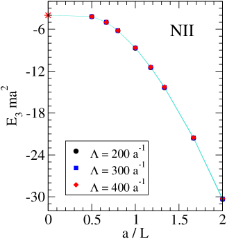
Figure 6: Variation of the trimer energy $E_{3}$ with the side length $L$ of the cubic volume for the states NI (left) and NII (right). Plotted are three datasets for different values of the cutoff parameter $\Lambda$, together with the $1/(\Lambda a)$ bands. The point $a/L=0$ corresponds to the infinite volume limit.

Figure 7: Variation of the trimer energy $E_{3}$ with the side length $L$ of the cubic volume for the states NIII. Plotted are three datasets for different values of the cutoff parameter $\Lambda$, together with the $1/(\Lambda a)$ bands.

The results for the states NI and NII are shown in Fig. 6 for box sizes between $L=2a$ and $L=a/2$. The results for the state NIII with box sizes between $L=8a$ and $L=a/2$ are depicted in Fig. 7. The values obtained with different cutoffs all agree with each other within the uncertainty bands indicating proper renormalization. Our findings are similar to those in the positive scattering length regime. All three states smoothly approach the infinite volume limit. As the box size becomes smaller the energy of the state is more and more diminished. The overall behavior is identical to the one in the positive scattering length case described in the previous section.

State	$E_{3}^{\infty}\,ma^{2}$	$E_{3}(L=a)\,ma^{2}$	$\delta_{rel}$	$L_{10\%}/a$	$L_{100\%}/a$
NI	$-9$	$-11.6$	29%	1.2	0.7
NII	$-4$	$-8.7$	118%	1.8	1.05
NIII	$-0.2$	$-6.7$	3250%	7.2	4.2

Table 5: For the states NI, NII and NIII, the infinite volume energy $E_{3}^{\infty}$ and the energy in a finite volume with side length $L=a$ are shown together with the relative deviation from the infinite volume value $\delta_{rel}=(E_{3}-E_{3}^{\infty})/E_{3}^{\infty}$. Also given are the box sizes leading to an energy shift of 10% and 100%, respectively.

The more deeply bound a state is in the infinite volume, the smaller is its spatial extent. Estimating the size via the formula $(-mE_{3}^{\infty})^{-1/2}$ yields $a/3$ for state NI, $a/2$ for state NII, and $2.2a$ for state NIII. A given finite volume should therefore affect state NII more than state NI, and state NIII should be the most affected. When considering a cubic volume with side length $L=a$, we find the energies given in Table 5. The relative deviation of state NI is indeed four times smaller than the shift for state NII and a hundred times smaller than the shift for the shallow state NIII. On the other hand, the box length $L_{10\%}$, for which the energy of each states deviates 10% from its infinite volume value, is smaller the more deeply bound a state is. These values are also given in Table 5.

As in the case of positive scattering length, we have investigated the dimensionless combination $r=-mE_{3}^{\infty}L_{10\%}^{2}$. From state NI, we obtain $r\approx 13$. This leads to the predictions $L_{10\%}=1.8a$ for state NII and $L_{10\%}=8a$ for state NIII in good agreement with the explicitly calculated values. Additionally, we form another dimensionless combination, $r^{\prime}=-mE_{3}^{\infty}L_{100\%}^{2}$, where $L_{100\%}$ is the box side length where the energy of the state is twice as large as the infinite volume value. For the three investigated states, this box size is also given in Table 5. From the value for the state NI, we get $r^{\prime}\approx 4.4$. From this value, we predict $L_{100\%}=1.05a$ for state NII and $L_{100\%}=4.7a$ for state NIII. Again, the value for state NII is as predicted, whereas the value for state NIII is about 10% off the prediction from universal scaling.

For states far away from the threshold, we expect that the regimes of negative and positive scattering length are governed by the same scaling factor. Therefore, the dimensionless combination $r$ should, for such deeply bound states, have a common value for both signs of $a$. For positive scattering lengths, state Ib is an example of a rather deeply bound state. For this state, we find $L_{10\%}=0.79a$ and from that $r=16.8$. For negative scattering lengths, we chose a state with $E_{3}^{\infty}=-27/(ma^{2})$ by setting $\Lambda_{\ast}a=8.54$. The energy of this state is shifted by 10% in a volume with side length $0.73a$, yielding $r=14.4$. The values of $r$ for the two signs of the scattering length are indeed close to each other for these two states. This behavior provides numerical evidence for the universality of finite volume effects for both positive and negative scattering lengths.

IV Conclusions

In this paper, we have extended our earlier studies of the Efimov spectrum in a cubic box with periodic boundary conditions Kreuzer:2008bi . The knowledge of the finite volume modifications of the spectrum is important in order to understand results from future 3-body lattice calculations. Using the framework of EFT, we have derived a general set of coupled sum equations for the Efimov spectrum in a finite volume.

Specializing to $\ell=0$, we have calculated the spectrum for both positive and negative scattering lengths and verified the renormalization in the finite box explicitly. We have removed the expansion for small finite volume shifts used in Ref. Kreuzer:2008bi and presented an extension that can be applied to arbitrarily large shifts. Typically, the binding of all three-body states increases as the box size is reduced. Moreover, we provided a more detailed discussion of the technical details and our numerical method. We have investigated the breakdown of the linear approximation in detail and find that the expansion is applicable as long as the finite volume shift in the energy is not larger than 15–20% of the infinite volume energy.

We have studied the spectrum for positive and negative scattering lengths in detail and provided numerical evidence for universal scaling of the finite volume effects. The scaling properties can be quantified by the dimensionless product $r$ of the three-body binding energy in the infinite volume limit and the square of the box length corresponding to a finite volume shift of ten percent of the infinite volume energy. For sufficiently deep states, we obtained numerical evidence that $r$ approaches a universal number for both signs of the scattering length. These findings suggest that the properties of deeper states in the finite volume can be obtained from a simple rescaling and do not require explicit calculations. A more detailed analysis of this issue along the lines of Braaten:2002sr is in progress.

For positive scattering lengths, we have investigated a spectrum of three states in the same physical system and studied the behavior of the shallowest state in the vicinity of the dimer energy which specifies the scattering threshold in the infinite volume. We found that this state drastically changes its behavior as a function of the box length once its energy becomes equal to the dimer energy. At this point the energy of the shallowest three-body state starts to grow and eventually becomes positive. The observed behavior is consistent with exponential suppression of the finite volume corrections below the dimer energy and power law suppression above.

The effect of an admixture of the $\ell=4$ partial wave has been investigated for two different three-body states for box sizes of the order of the size of the state. For a generic state well separated from threshold, we found corrections of the order of a few percent for volumes that are about three times larger than the state itself. For the state closest to threshold, the effect of this admixture turns out to be surprisingly small for volumes about twice as large as the state and was found to be less than $1\%$. As the finite cutoff corrections for this state are about the same size, a more quantitative study requires an improved treatment of these corrections. Such studies are in progress.

Finally, our method should be extended to the three-nucleon system. This requires also the inclusion of higher order corrections in the EFT and finite temperature effects as lattice calculations will inevitably be performed at a small, but non-zero, temperature. Work in these directions is in progress. With high statistics lattice QCD simulations of three-baryon systems within reach Beane:2009gs , the calculation of the structure and reactions of light nuclei appears now feasible in the intermediate future. Our results demonstrate that the finite volume corrections for such simulations are calculable and under control. This also opens the possibility to test the conjecture of an infrared limit cycle in QCD for quark masses slightly larger than the physical values Braaten:2003eu .

Appendix A Numerical treatment

In this appendix, we give some details on the numerical solution of Eqs. (17, 19). The starting point for a first numerical treatment of the formalism is the homogeneous integral equation

$$F_{0}(p)=\frac{4}{\pi}\int_{0}^{\Lambda}\mathrm{d}y\,y^{2}Z_{E}^{(0)}(p,y)\tau_{E}(y)\bigg{(}1+\sum_{\begin{subarray}{c}\vec{n}\in\mathbb{Z}^{3}\\ \vec{n}\neq 0\end{subarray}}\frac{\sin(L|\vec{n}|y)}{L|\vec{n}|y}\bigg{)}F_{0}(y).$$ (21)

The first step is to transform this equation into a finite-dimensional problem. Due to the oscillatory nature of the integrand, it is not sensible to use a finite number of sampling points. Therefore, a set of basis functions will be used. The choice of the basis functions is guided by the knowledge of the bound-state amplitude in the infinite volume case. Asymptotically, the amplitude in the infinite volume behaves like Bedaque:1998kg ; Braaten:2004rn

$$F_{0}(p)\rightarrow\frac{1}{p}\cos\left(s_{0}\log(p/p_{\ast})\right),$$

with the universal number $s_{0}=1.00624\dots$ and a momentum scale $p_{\ast}$. The bound-state amplitude obtained by the infinite volume formalism has precisely such a form, with only a few zeros in the interval $\left[0;\Lambda\right]$ (See, e.g., Ref. Bedaque:1998kg ). Therefore, the basis functions $\xi_{i}$ are chosen as Legendre functions $P_{i}$ with logarithmic arguments as

$$\xi_{i}(p)=\frac{1}{p}P_{i}(2\log_{2}(p/\Lambda+1)-1).$$ (22)

These basis functions are orthogonal with respect to a suitably chosen scalar product:

$$\int_{0}^{\Lambda}\mathrm{d}p\,\frac{p^{2}}{p+\Lambda}\xi_{i}(p)\xi_{j}(p)=(\log 2)\,\frac{1}{2i+1}\delta_{ij}.$$ (23)

The amplitude $F_{0}$ in Eq. (21) is replaced by its expansion in the basis functions $\sum_{j=0}^{\infty}f_{j}\xi_{j}(p)$ and the $i$th component is projected out using the scalar product. The resulting equation

$$\frac{\log 2}{2i+1}f_{i}=\sum_{j=0}^{\infty}K_{ij}(E)f_{j},$$ (24)

with

$$K_{ij}{(E)}=\frac{4}{\pi}\int_{0}^{\Lambda}\mathrm{d}y\,y^{2}\bigg{[}\int_{0}^{\Lambda}\mathrm{d}p\,\frac{p^{2}}{p+\Lambda}\xi_{i}(p)Z_{E}^{(0)}(p,y)\bigg{]}\tau_{E}(y)\bigg{(}1+\sum_{\begin{subarray}{c}\vec{n}\in\mathbb{Z}^{3}\\ \vec{n}\neq 0\end{subarray}}\frac{\sin(L|\vec{n}|y)}{L|\vec{n}|y}\bigg{)}\xi_{j}(y),$$ (25)

can be interpreted as a matrix equation when truncating the set of basis functions.

A non-trivial solution of Eq. (24) can be found if the condition

$$\det\left[K_{ij}{(E)}-\frac{\log 2}{2i+1}\delta_{ij}\right]=0$$ (26)

is fulfilled. Values of $E$, for which this is the case, are then considered as trimer energies in the finite volume. This is only a valid interpretation if the truncation of the basis and the neglect of the higher partial waves induce only small corrections for the result.

The value of the parameter $E$ for which the condition (26) is satisfied is found via a root finding algorithm. This requires the calculation of $K_{ij}(E)$ in each iteration. To save numerical effort, it is possible to expand the kernel around the binding energy in infinite volume if the shift in the binding energy is small. The expansion is done up to first order:

$$K_{ij}(E)\approx K_{ij}(E^{\infty})+\left.\frac{\mathrm{d}K_{ij}}{\mathrm{d}E}\right|_{E=E^{\infty}}\cdot(E-E^{\infty}),\quad\mbox{ for }\frac{E-E^{\infty}}{E^{\infty}}\ll 1.$$ (27)

This expansion has been used to obtain the results in Kreuzer:2008bi . It is applicable as long as the finite volume shift in the energy is not larger than 15–20% of the infinite volume energy.

In the following, details on the numerical methods used to calculate the kernel matrix elements as defined in Eq. (25) are presented. The integration over $p$ is performed using a logarithmically distributed Gauss-Legendre quadrature with 64 points.

The integrand of the $y$-integration is strongly oscillating due to the $\sin(L|\vec{n}|y)$ term. Therefore, this integral is evaluated using the Fast Fourier Transformation technique (FFT). The computation of Fourier-type integrals via FFT is explained in detail in NumRep:07 . The sampling for the FFT is the most time-consuming part of the calculation. The number of points to sample, $M$, is determined by the highest “frequency” that is to be accessed. The frequencies in the present case are the values of $L|\vec{n}|$. The highest possible frequency is connected to $M$ and the integration range $\Lambda$ by

$$L|\vec{n}_{\mathrm{max}}|\,\frac{\Lambda}{M}<\pi\quad\Rightarrow\quad M>\frac{L|\vec{n}_{\mathrm{max}}|\Lambda}{\pi}.$$ (28)

For realistic values of these parameters, namely box sizes of a few $a$, an $|\vec{n}_{\mathrm{max}}|$ of about 3000 and cutoff values of several hundred $a^{-1}$, a typical value for $M$ is $2^{20}$ or about one million sampled points.

A summation over three-dimensional integer vectors of a quantity depending only on the absolute values involves substantial double counting when naïvely done. To circumvent this problem, an ordered list with all absolute values that are possible for vectors in $\mathbb{Z}^{3}$ and their multiplicity has been created. The result of the summation can be viewed as converged when going to absolute values of about $R\approx 5000$ (see the example in Fig. 8). For radii $R$ from about 2000 on, the intermediate sums oscillate around the converged result. To reduce runtime, the result of the summation has been calculated as a mean of 15 intermediate sums for radii from 2750 to 3500.

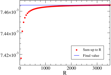
Figure 8: Convergence of the sum over vectors in $\mathbb{Z}^{3}$ as a function of the radius $R$.

The calculation of the matrix elements has been performed on the cluster of the HISKP at the University of Bonn. As already stated above, the number of sampling points for the FFT is the parameter with the largest influence on the runtime. When using the expanded integral kernel, the matrix and the derivative matrix have to be calculated only once. For a typical sample size of $2^{20}$, this takes about 100 minutes. When going to smaller volumes, the shifts in the binding energy become larger and the Taylor expansion of the integral kernel breaks down. In this case, it is inevitable to recalculate the kernel matrix in each iteration of the root finding algorithm. This amounts to 10 to 15 evaluations of the kernel matrix and a runtime of 8 to 10 hours per data point.

References

- (1) E. Braaten and H.-W. Hammer, Phys. Rept. 428, 259 (2006) [arXiv:cond-mat/0410417].
- (2) L. Platter, Few Body Syst. 46, 139 (2009) [arXiv:0904.2227 [nucl-th]].
- (3) V. Efimov, Phy. Lett. 33B, 563 (1970).
- (4) V. Efimov, Sov. J. Nucl. Phys. 29, 546 (1979).
- (5) P.F. Bedaque, H.-W. Hammer, and U. van Kolck, Phys. Rev. Lett. 82, 463 (1999) [arXiv:nucl-th/9809025]; Nucl. Phys. A 646, 444 (1999) [arXiv:nucl-th/9811046].
- (6) T. Kraemer, M. Mark, P. Waldburger, J.G. Danzl, C. Chin, B. Engeser, A.D. Lange, K. Pilch, A. Jaakkola, H.-C. Nägerl, and R. Grimm, Nature 440, 315 (2006).
- (7) S. Knoop, F. Ferlaino, M. Mark, M. Berninger, H. Schoebel, H.-C. Naegerl, R. Grimm Nature Physics 5, 227 (2009) [arXiv:0807.3306 [cond-mat]].
- (8) T. B. Ottenstein, T. Lompe, M. Kohnen, A. N. Wenz, S. Jochim, Phys. Rev. Lett. 101, 203202 (2008) [arXiv:0806.0587 [cond-mat]].
- (9) J. H. Huckans, J. R. Williams, E. L. Hazlett, R. W. Stites, K. M. O’Hara, Phys. Rev. Lett. 102, 165302 (2009) [arXiv:0810.3288 [physics.atom-ph]].
- (10) G. Barontini, C. Weber, F. Rabatti, J. Catani, G. Thalhammer, M. Inguscio, F. Minardi, Phys. Rev. Lett. 103, 043201 (2009) [arXiv:0901.4584v1 [cond-mat.other]].
- (11) N. Gross, Z. Shotan, S. Kokkelmans, L. Khaykovich, Phys. Rev. Lett. 103, 163202 (2009) [arXiv:0906.4731v1 [cond-mat.other]].
- (12) M. Zaccanti, B. Deissler, C. D’Errico, M. Fattori, M. Jona-Lasinio, S. Müller, G. Roati, M. Inguscio, G. Modugno, Nature Physics 5, 586 (2009) [arXiv:0904.4453v1 [cond-mat.quant-gas]].
- (13) D. L. Canham and H.-W. Hammer, Eur. Phys. J. A 37, 367 (2008) [arXiv:0807.3258 [nucl-th]] and references therein.
- (14) K.G. Wilson, Nucl. Phys. Proc. Suppl. 140, 3 (2005) [arXiv:hep-lat/0412043].
- (15) S.R. Beane, P.F. Bedaque, M.J. Savage, and U. van Kolck, Nucl. Phys. A 700, 377 (2002) [arXiv:nucl-th/0104030].
- (16) S.R. Beane and M.J. Savage, Nucl. Phys. A 717, 91 (2003) [arXiv:nucl-th/0208021]; Nucl. Phys. A 713, 148 (2003) [arXiv:nucl-th/0206113].
- (17) E. Epelbaum, U.-G. Meißner, and W. Glöckle, Nucl. Phys. A 714, 535 (2003) [arXiv:nucl-th/0207089].
- (18) E. Braaten and H.-W. Hammer, Phys. Rev. Lett. 91, 102002 (2003) [arXiv:nucl-th/0303038].
- (19) E. Epelbaum, H.-W. Hammer, U.-G. Meißner and A. Nogga, Eur. Phys. J. C 48, 169 (2006) [arXiv:hep-ph/0602225].
- (20) H.-W. Hammer, D.R. Phillips and L. Platter, Eur. Phys. J. A 32, 335 (2007) [arXiv:0704.3726 [nucl-th]].
- (21) S. R. Beane, P. F. Bedaque, K. Orginos and M. J. Savage, Phys. Rev. Lett. 97, 012001 (2006) [arXiv:hep-lat/0602010].
- (22) S. R. Beane et al., Phys. Rev. D 80 (2009) 074501 arXiv:0905.0466 [hep-lat].
- (23) S. R. Beane, K. Orginos and M. J. Savage, Int. J. Mod. Phys. E 17, 1157 (2008) [arXiv:0805.4629 [hep-lat]].
- (24) S. R. Beane, P. F. Bedaque, A. Parreno and M. J. Savage, Phys. Lett. B 585, 106 (2004) [arXiv:hep-lat/0312004].
- (25) S. Tan, Phys. Rev. A 78, 013636 (2008) [arXiv:0709.2530 [cond-mat]].
- (26) S. R. Beane, W. Detmold and M. J. Savage, Phys. Rev. D 76, 074507 (2007) [arXiv:0707.1670 [hep-lat]].
- (27) W. Detmold and M. J. Savage, Phys. Rev. D 77, 057502 (2008) [arXiv:0801.0763 [hep-lat]].
- (28) S. R. Beane, W. Detmold, T. C. Luu, K. Orginos, M. J. Savage and A. Torok, Phys. Rev. Lett. 100 (2008) 082004 [arXiv:0710.1827 [hep-lat]].
- (29) W. Detmold, M. J. Savage, A. Torok, S. R. Beane, T. C. Luu, K. Orginos and A. Parreno, Phys. Rev. D 78, 014507 (2008) [arXiv:0803.2728 [hep-lat]].
- (30) W. Detmold, K. Orginos, M. J. Savage and A. Walker-Loud, Phys. Rev. D 78, 054514 (2008) [arXiv:0807.1856 [hep-lat]].
- (31) L. Pricoupenko and Y. Castin, J. Phys. A 40, 12863 (2007) [arXiv:0705.1502 [cond-mat]].
- (32) M. Lüscher, Nucl. Phys. B 354, 531 (1991).
- (33) M. Lüscher, Nucl. Phys. B 364, 237 (1991).
- (34) V. Bernard, U.-G. Meißner and A. Rusetsky, Nucl. Phys. B 788, 1 (2008) [arXiv:hep-lat/0702012].
- (35) V. Bernard, M. Lage, U.-G. Meißner and A. Rusetsky, JHEP 08, 024 (2008) [arXiv:0806.4495 [hep-lat]].
- (36) S. Kreuzer and H.-W. Hammer, Phys. Lett. B 673, 260 (2009) [arXiv:0811.0159 [nucl-th]].
- (37) F. C. von der Lage and H. A. Bethe, Phys. Rev. 71, 612 (1947).
- (38) S. L. Altmann and A. P. Cracknell, Rev. Mod. Phys. 37, 19 (1965).
- (39) E. Braaten, H. W. Hammer and M. Kusunoki, Phys. Rev. A 67 (2003) 022505 [arXiv:cond-mat/0201281].
- (40) W. H. Press, S. A. Teukolsky, W. T. Vetterling, B. P. Flannery. Numerical Recipes: The Art of Scientific Computing, Third Edition, Cambridge University Press, 2007.