Applications of Computer Simulations and Statistical Mechanics in Surface Electrochemistry

Abstract

We present a brief survey of methods that utilize computer simulations and quantum and statistical mechanics in the analysis of electrochemical systems. The methods, Molecular Dynamics and Monte Carlo simulations and quantum-mechanical density-functional theory, are illustrated with examples from simulations of lithium-battery charging and electrochemical adsorption of bromine on single-crystal silver electrodes.

I Introduction

The interface between a solid electrode and a liquid electrolyte is a complicated many-particle system, in which the electrode ions and electrons interact with solute ions and solvent ions or molecules through several channels of interaction, including forces due to quantum-mechanical exchange, electrostatics, hydrodynamics, and elastic deformation of the substrate. Over the last few decades, surface electrochemistry has been revolutionized by new techniques that enable atomic-scale observation and manipulation of solid-liquid interfaces KOLB02 ; TANS06 , yielding novel methods for materials analysis, synthesis, and modification. This development has been paralleled by equally revolutionary developments in computer hardware and algorithms that by now enable simulations with millions of individual particles VASH06 , so that there is now significant overlap between system sizes that can be treated computationally and experimentally.

In this chapter, we discuss some of the methods available to study the structure and dynamics of electrode-electrolyte interfaces using computers and techniques based on quantum and statistical mechanics. These methods are illustrated by some recent applications. The rest of the chapter is organized as follows. In Sec. II, we present fully three-dimensional, continuum simulations by Molecular Dynamics (MD) of ion intercalation during charging of Lithium-ion batteries. In Sec. III, we discuss the simplifications that are possible by mapping a chemisorption problem onto an effective lattice-gas (LG) Hamiltonian , and in Sec. IV we demonstrate how input parameters for a statistical-mechanical LG model can be estimated from quantum-mechanical density-functional theory (DFT) calculations. Section V is devoted to a discussion of Monte Carlo (MC) simulations, both for equilibrium problems (Sec. V.1) and for dynamics (Sec. V.2). As an example of the latter, we present in Sec. VI a simulational demonstration of a method to classify surface phase transitions in adsorbate systems, which is an extension of standard cyclic voltammetry (CV): the Electrochemical First-order Reversal Curve (EC-FORC) method. A concluding summary is given in Sec. VII.

II Molecular Dynamics Simulations of Ion Intercalation in Lithium Batteries

The charging process in Lithium-ion batteries is marked by the intercalation of Lithium ions into the graphite anode material. Here we present MD simulations of this process and suggest a new charging method that has the potential for shorter charging times, as well as the possibility of providing higher power densities.

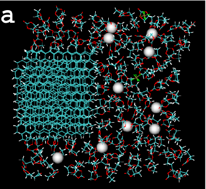
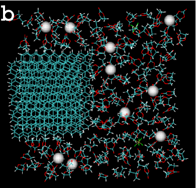
Figure 1: (a) Snapshot of the model system containing four graphite sheets, two PF${}_{6}^{-}$ ions and ten Li⁺ ions (spheres), solvated in $69$ propylene carbonate and $87$ ethylene carbonate molecules after reaching constant volume in the $NPT$ ensemble. (b) Snapshot after $200$ ns MD simulation. The ensemble is the $NVT$ ensemble. The system has periodic boundary conditions and is simulated at one atm and 300 K. Top view, perpendicular to the plane of the graphite sheets.

II.1 Molecular Dynamics and Model System

Molecular Dynamics is based on solving the classical equations of motion for a system of $N$ atoms interacting through forces derived from a potential-energy function Allen:92 ; Haile:92 ; Rapaport:04 ; VOTE97 ; VOTE97B . From the potential energy $E_{\rm P}$, the force on the $i$th atom, $F_{i}$, is calculated. Thus, the equation of motion is

$$F_{i}(t)=-\frac{\partial E_{\rm P}}{\partial r_{i}}=m_{i}\frac{\partial v_{i}}{\partial t}=m_{i}\frac{\partial^{2}r_{i}}{\partial t^{2}}$$ (1)

where $r_{i}$, $v_{i}$, and $m_{i}$ are the position, velocity, and mass of the $i$th atom, respectively. Consequently, the quality of the simulations strongly depends on the ability of the classical force field to reasonably describe the atomistic behavior.

The newly developed General Amber Force Field (GAFF) GAFF:04 was used to approximate the bonded interactions of all the simulation molecules, while the simulation package Spartan (Wave-function, Inc., Irvine, CA) was used at the Hartree-Fock/6-31g* level to obtain the necessary point charges for each of the atoms. To simulate a charging field, the charge on the carbon atoms of the graphite sheets was set to $-0.0125$ e per atom. The bonded (first three terms of Eq. (2)) and non-bonded (last term) interactions in the AMBER Force Field are represented by the following potential-energy function:

$$E_{\rm P}=\sum_{\rm bonds}K_{r}(r-r_{eq})^{2}+\sum_{\rm angles}K_{\theta}(\theta-\theta_{eq})^{2}+\sum_{\rm dihedrals}{V_{n}\over 2}[1+{\rm cos}(n\phi-\gamma)]+\sum_{i<j}\left[{A_{ij}\over R_{ij}^{12}}-{B_{ij}\over R_{ij}^{6}}+{q_{i}q_{j}\over\epsilon R_{ij}}\right]$$ (2)

where $K_{\rm r}$, $K_{\theta}$ and $V_{n}$ are the bond stretching, bending and torsional constants respectively, the constants $A$ and $B$ define van der Waals’ interactions between unbonded atoms, and $\epsilon$ is the electrostatic permittivity. The simulation package NAMD NAMD was used for the MD simulations, while the graphics package VMD VMD was used for visualization and analysis of the simulation results.

The model system representing the anode half-cell is composed of four graphite sheets (anode) containing $160$ carbon atoms each, two PF${}_{6}^{-}$ ions, and ten Li⁺ ions, solvated in an electrolyte made of $69$ propylene carbonate and $87$ ethylene carbonate molecules (see Fig. 1(a)). The graphite sheets were fixed from one side by keeping the positions of the edge carbon atoms fixed.

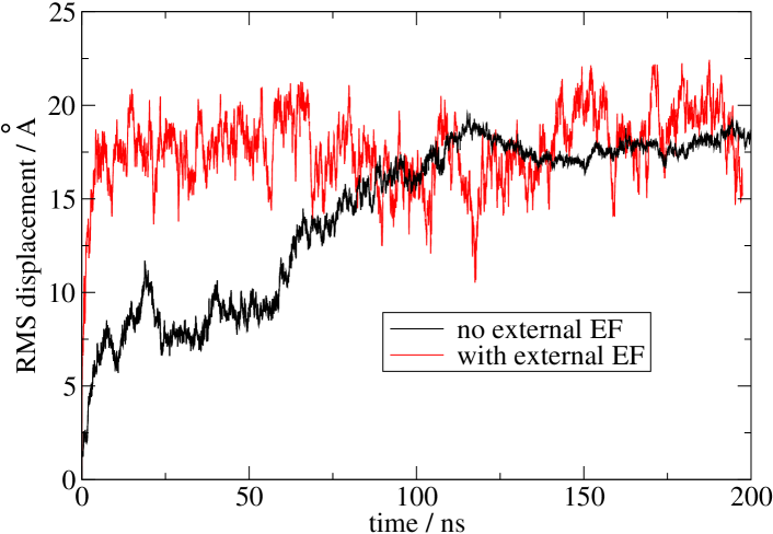
Figure 2: Root-mean-square displacement of Lithium ions as a function of time. Diffusion is much faster with the additional oscillating electric field (amplitude 5 kCal/mol, frequency 25 GHz).

II.2 Simulations and Results

After energy minimization, the simulations were run at constant pressure using a Langevin piston Nosé-Hoover method Martyna:94 ; Feller:95 as implemented in the NAMD software package until the system has reached its equilibrium volume at a pressure of $1$ atm and 300 K in the $NPT$ (constant particle number, pressure, and temperature) ensemble. The system’s behavior was then simulated for $200$ ns ($100$ million steps) in the $NVT$ (constant particle number, volume, and temperature) ensemble. Two observations were made: first, the Li⁺ ions stayed randomly distributed within the electrolyte, and second, none of the Li⁺ ions had intercalated between the graphite sheets after $200$ ns (see Fig. 1(b)).

While the Lithium ions do not intercalate within the simulation time given above, it is expected that given enough time they will move towards the graphite sheets and get intercalated. To test whether intercalation is possible in such a model system, one of the Lithium ions was positioned between the graphite sheets at the beginning of a simulation, and we observed whether it diffused out from between the sheets. The Lithium ion stayed intercalated, even after $400$ ns.

In order for intercalation to occur, the Lithium ion has first to diffuse within the electrolyte until it reaches the graphite electrode. Consequently, faster diffusion would result in faster intercalation and shorter charging time. In order to increase the diffusion of Lithium ions in the electrolyte, we explored a new charging method. In addition to the charging field due to the fixed charge on the graphite carbons, an external oscillating square-wave field (amplitude 5 kCal/mol, frequency 25 GHz) was applied in the direction perpendicular to the plane of the graphite sheets. Not only does this additional field increase diffusion, but also some of the Lithium ions intercalate into the graphite sheets within an average time of about 50 ns. Figure 2 shows a plot of the root-mean-square displacement of Lithium ions as a function of time for a system with and without an applied external field. The increased diffusion and intercalation indicate that a charging protocol involving an oscillating field may decrease the charging time and possibly increase the battery’s power density.

III Lattice-gas Models of Chemisorbed Systems

As mentioned in the Introduction, even the simplest electrosorption systems are extremely complicated. This complexity means that a comprehensive theoretical description that enables predictions for phenomena on macroscopic scales of time and space is still generally impossible with present-day methods and technology. (Note that MD simulations, such as those presented in Sec. II, are only possible up to times of a few hundred nanoseconds.) Therefore, it is necessary to use a variety of analytical and computational methods and to study various simplified models of the solid-liquid interface. One such class of simplified models are Lattice-gas (LG) models, in which chemisorbed particles (solutes or solvents) can only be located at specific adsorption sites, commensurate with the substrate’s crystal structure. This can often be a very good approximation, as for instance for halides on the (100) surface of Ag, for which it can be shown that the adsorbates spend the vast majority of their time near the four-fold hollow surface sites MITC02 . A lattice-gas approximation to such a continuum model, appropriate for chemisorption of small molecules or ions HUCK90 ; BLUM94A ; BLUM96 ; GAMB93B ; RIKV95 ; JZHA95B , is defined by the discrete, effective grand-canonical Hamiltonian,

$${\cal H}_{\rm LG}=\sum_{n}[-\Phi^{(n)}\sum_{\langle ij\rangle}^{(n)}c_{i}c_{j}]+{\cal H}_{3}-\bar{\mu}\sum_{i}c_{i}\;.$$ (3)

Here, the lattice sites $i$ are the preferred adsorption sites (the minima of the continuous corrugation potential), and $c_{i}$ is a local occupation variable, with 1 corresponding to an adsorbed particle and 0 to a solvated site. The sums $\sum_{\langle ij\rangle}^{(n)}$ and $\sum_{i}$ run over all $n$th-neighbor pairs and over all adsorption sites, respectively, $\Phi^{(n)}$ is the effective $n$th-neighbor pair interaction, and $\sum_{n}$ runs over the interaction ranges. The term ${\cal H}_{3}$ contains multi-particle interactions EINS91 ; HYLD05 ; STAS06 . The sign convention is such that $\phi<0$ implies repulsion, and $\bar{\mu}>0$ favors adsorption. Equation (3) is also easily generalized to multiple species RIKV88B ; COLL89 .

To connect the electrochemical potentials to the concentrations in bulk solution of species X, [X], and the electrode potential, $E$, one has (in the dilute-solution approximation)

$$\bar{\mu}_{\rm x}(T,[{\rm X}],E)=\bar{\mu}_{\rm x}^{0}+k_{\rm B}T\ln([{\rm X}]/[{\rm X}]^{0})-e\int_{E^{0}}^{E}\gamma_{\rm x}(E^{\prime}){\rm d}E^{\prime}\;,$$ (4)

where $k_{\rm B}$ is Boltzmann’s constant, $T$ the temperature, $e$ the elementary charge, and $\gamma_{\rm x}(E)$ the electrosorption valency SCHM96 ; VETT72A ; VETT72B ; RIKV07 of X. The importance of the integral over the potential-dependent electrosorption valency (rather than just the product $e\gamma_{\rm x}(E)E$) analogous to the case of potential-independent $\gamma_{\rm x}$) was pointed out in Ref. HAMA05B . The quantities superscripted “0” are reference values that include local binding energies. The interaction constants and electrosorption valencies are effective parameters influenced by several physical effects, including electronic structure EINS91 ; HYLD05 ; STAS06 , surface deformation, (screened) electrostatic interactions KOPE98 ; GLOS93A ; GLOS93B , and the fluid electrolyte BLUM90 ; IGNA98 . The density conjugate to $\bar{\mu}_{\rm x}$ is the coverage relative to the number $N$ of adsorption sites,

$$\Theta_{\rm X}=N^{-1}\sum_{i}c_{i}\;.$$ (5)

IV Calculation of Lattice-gas Parameters by Density Functional Theory

There are many methods to estimate lattice-gas parameters. One of these is comparison of MC simulations (see Sec. V) of a LG model with experimental adsorption isotherms. For detailed descriptions of this method we refer to Refs. KOPE98 ; BROW99A ; MITC00A ; MITC00C ; HAMA03 ; HAMA05B . Here we instead concentrate on the purely theoretical method based on quantum-mechanical DFT calculations STAS06 .

DFT is the most widely used method to calculate ground-state properties of many-electron systems. It is based on the Hohenberg-Kohn theorem, which states that all properties of the many-particle ground state can be expressed in terms of the ground-state electron charge-density distribution Hohenberg and leads to the Kohn-Sham equations for single-particle wave functions Kohn . These are second-order differential equations, which include potential terms due to the ions and the classical Coulomb repulsive energy between the electrons, as well as the electronic exchange-correlation energy, and they are solved self-consistently. For surface structural studies, DFT is usually performed using pseudopotentials with slab models and plane-wave basis sets. The slab consists of a finite number of atomic layers, periodic in the direction parallel to the surface, which can either be repeated periodically in the third direction (separated by a vacuum interval), or not. The fluid solvent can be considered either as an effective continuum, or by molecular models.

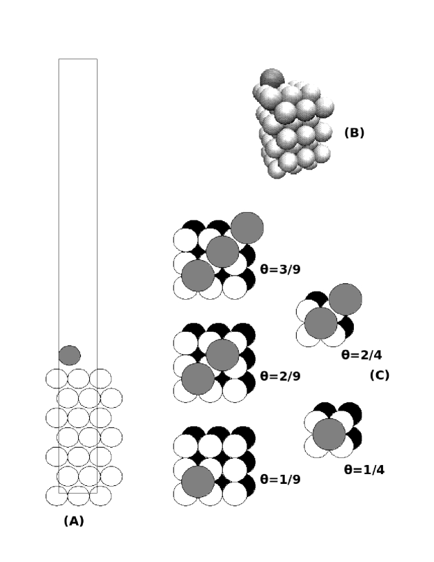
Figure 3: (A) Cross section of a $3\times 3$ supercell with $\Theta=1/9$. (B) Three-dimensional representation of the same cell and coverage. (C) Top view of a $3\times 3$ surface and a $2\times 2$ surface with various coverages.

Here we present preliminary results on a DFT calculation of lateral interaction constants pertaining to a lattice-gas model for the adsorption of Br on single-crystal Ag(100) surfaces HAMA03 ; HAMA04 ; RIKV07 ; MITC00A ; MITC00C . The lattice-gas model is represented by Eq. (3) on a square lattice with lattice constant $a=2.95$ Å, $\mathcal{H}_{3}=0$, infinitely repulsive interactions for adparticles at nearest-neighbor sites, and the long-range repulsion

$$\phi_{ij}=\frac{(\sqrt{2})^{3}}{r_{ij}^{3}}\phi_{\rm nnn}\;\;\;{\rm for}\;\;\;r_{ij}\geq\sqrt{2}\;,$$ (6)

which is compatible with dipole-dipole interactions or elastically mediated interactions. (Here, $r_{ij}$ is given in units of $a$.) Since the DFT calculations are performed in the canonical ensemble (fixed adsorbate coverage), $\bar{\mu}$ in Eq. (3) is replaced by the binding energy of a single adparticle, $E_{\rm b}$.

We prepared slabs with seven metal layers, which were placed inside a supercell with periodic boundary conditions. Two different sizes of supercells were used: a $2\times 2$ supercell with the size of $2a\times 2a\times 36.95$ Å, and a $3\times 3$ supercell with the size of $3a\times 3a\times 36.95$ Å. The vacuum region above the surface was twice the thickness of the slab, and the orientation of the surface normal was in the $z$ direction. One, two, and three Br atoms were placed on the $3\times 3$ surface to represent coverages $\Theta=1/9$, $2/9$, and $1/3$. Two Br atoms were placed on the $2\times 2$ surface to represent $\Theta=1/2$, and one to represent $\Theta=1/4$. Supercells with different coverages of Br are shown in Fig. 3.

The DFT calculations were performed using the Vienna Ab Initio Simulation Package (VASP) KRES93 ; KRES96A ; KRES96B . The basis set was plane-wave, with the generalized gradient-corrected exchange-correlation function Perdew2 ; Perdew1 , and Vanderbilt pseudopotentials Vanderbilt . The $k$-point mesh was generated using the Monkhorst method MONK76 with a $5\times 5\times 1$ grid for the $3\times 3$ cells and a $7\times 7\times 1$ grid for the $2\times 2$ cells. All calculations were done on a $54\times 54\times 192$ real-space grid.

Individual DFT calculations provide total energies, $E$, and charge densities, $\rho(\vec{x})$. The adsorption energy $E_{\rm ads}$ for a single adatom and the corresponding charge-transfer function $\Delta\rho(\vec{x})$ are obtained from calculations of the adsorbed system and isolated slab and atoms as follows:

$$E_{\rm ads}=\left[E_{\rm syst}-E_{\rm slab}\right]/N_{\rm ads}-E_{\rm Br}$$ (7)

and MITC04

$$\Delta\rho(\vec{x})=[\rho(\vec{x})_{\rm syst}-\rho(\vec{x})_{\rm slab}]/N_{\rm ads}-\rho(\vec{x})_{\rm Br}\;,$$ (8)

where $N_{\rm ads}=N\Theta$ is the number of adsorbed Br atoms in the cell, and the quantities subscripted Br refer to a single, isolated Br atom.

Since the system is electrically neutral, the integral over space of $\Delta\rho(\vec{x})$ vanishes. The surface dipole moment is defined as

$$p=\int z\Delta\rho(z)dz\;.$$ (9)

Kohn and Lau KOHN76 have shown that the non-oscillatory part of the dipole-dipole interaction energy between adsorbates separated by a distance $R$ behaves as

$$\phi_{\rm dip-dip}=\frac{2p_{a}p_{b}}{4\pi\epsilon_{0}R^{3}}$$ (10)

for large $R$ (in our case larger than the nearest-neighbor distance). This result is twice what one might naïvely expect. Thus, the next-nearest-neighbor interaction constant from Eq. (6) would be

$$\phi_{\rm{dip-dip~{}nnn}}=\frac{2p^{2}}{4\pi\epsilon_{0}R^{3}_{\rm{nnn}}}$$ (11)

with $p$ obtained from the DFT by Eq. (9). This estimate, which depends on $\Theta$, is included in Fig. 4 as solid circles.

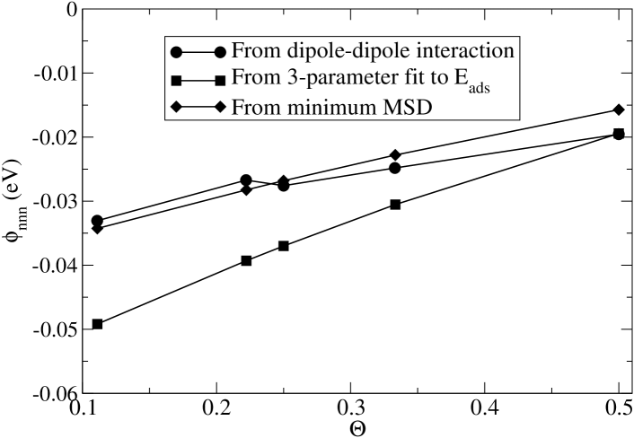
Figure 4: Three different estimates of the LG interaction constant $\phi_{\rm nnn}$. Circles: Based on Eq. (10) with the dipole moment $p$ directly obtained from the DFT calculation. Squares: Based on a three-parameter fit to the DFT adsorption energy $E_{\rm ads}$ as described in Eq. (12). Diamonds: Based on minimizing mean-square deviations (MSD) from the estimate based on the DFT dipole moment $p$, constrained to retain a low value of the $\chi^{2}$ from the fit to $E_{\rm ads}$. See discussion in the text.

Alternatively, the interaction constant $\phi_{\rm nnn}$ in the LG Hamiltonian, Eq. (3), can be estimated by performing a nonlinear least-squares fit of the $\Theta$-dependent DFT adsorption energy $E_{\rm ads}$ in Eq. (7) to

$$E_{\rm ads}=-\phi_{\rm nnn}\Sigma_{\Theta}-E_{\rm b}\Theta$$ (12)

with $\phi_{\rm nnn}=A(1+B\Theta)^{2}$, using the three fitting parameters $A$, $B$, and $E_{\rm b}$. This is consistent with the theoretical prediction of Eq. (11) with a dipole moment that depends linearly on $\Theta$. The quantity

$$\Sigma_{\Theta}=\frac{(\sqrt{2})^{3}}{N}\sum_{i<j}\frac{c_{i}c_{j}}{r_{ij}^{3}}$$ (13)

can be calculated numerically to any given accuracy for a particular coverage and adsorbate configuration. This estimate for $\phi_{\rm nnn}$ is included in Fig. 4 as solid squares. It does not agree particularly closely with the result obtained from the dipole moments. However, we found that the $\chi^{2}$ of the fit, considered as a function of the fitting parameters, was characterized by an extremely wide and shallow basin surrounding its minimum. We therefore further minimized the mean-square deviation (MSD) between the values of $\phi_{\rm nnn}$ obtained from this fitting procedure and those obtained directly from Eq. (11) with the DFT values for $p$ within the three-dimensional parameter region for which the original $\chi^{2}$ was close to its minimum. This procedure gave significantly improved consistency between the two estimates for $\phi_{\rm nnn}$, without a significant increase in $\chi^{2}$. The final result is shown as solid diamonds in Fig. 4, and the corresponding parameters are listed in Table 1.

The average value of $\phi_{\rm nnn}$ obtained by this method is consistent with that found by fitting equilibrium MC simulations (see Sec. V.1) to experimental adsorption isotherms in aqueous solution (approximately $-21$ meV). However, no significant coverage dependence was found in the analysis of the experimental data HAMA03 ; HAMA05B . It is not surprising that results from in situ experiments and in vacuo DFT calculations should show some differences, and we find it encouraging that the average results are consistent. Application of the method described here to Cl/Ag(100) gave less consistent results than for Br, possibly indicating that the effective interactions for Cl are not purely dipole-dipole in nature JUWO08 .

Table 1: Results for the fits of the $\Theta$-dependent lattice-gas interaction constant $\phi_{\rm nnn}$ according to the two methods described in the text. Here, $\nu$ is the number of degrees of freedom (number of data points minus number of parameters, here equal to 2) for the initial nonlinear least-squares fit of $\phi_{\rm nnn}$ to the DFT adsorption energy $E_{\rm ads}$, while MSD is the mean-square deviation between this estimate and the estimate obtained directly from the DFT dipole moment. Minimizing MSD within the basin of low $\chi^{2}$ significantly reduces MSD (see the greatly improved agreement in Fig. 4) without significantly increasing $\chi^{2}$.

Method	$A$	$B$	$E_{\rm b}$	$\chi^{2}/\nu$	MSD/$\nu$
Min. $\chi^{2}$	$-6.017\times 10^{-2}$	$-0.8632$	3.102	$2.362\times 10^{-5}$	$1.803\times 10^{-4}$
Min. MSD	$-4.085\times 10^{-2}$	$-0.7595$	3.070	$2.675\times 10^{-5}$	$7.692\times 10^{-6}$

V Monte Carlo Simulations

V.1 Equilibrium Monte Carlo

As a method to obtain equilibrium properties of a system described by a particular Hamiltonian, MC is more accurate than mean-field approximations, especially for low-dimensional systems near phase transitions BROW99A ; LAND00 . This is an effect of fluctuations which, while ignored or underestimated by mean-field methods, are very important in two-dimensional systems. Given the rapid evolution of computers and the relative ease of programming of MC codes, this is our method of choice for equilibrium and dynamic studies of both lattice-gas and continuum models.

The goal of an equilibrium MC code is to bring the system to equilibrium as rapidly as possible, and then sample the equilibrium distribution as efficiently as possible. The only requirement is that the transition rates between two configurations $c$ and $c^{\prime}$ satisfy detailed balance,

$${{\cal R}({c^{\prime}}\rightarrow{c})}/{{\cal R}({c}\rightarrow{c^{\prime}})}=\exp{\left[-\left({{\cal H}({c})-{\cal H}({c^{\prime}})}\right)/{k_{\rm B}T}\right]}\;.$$ (14)

This result applies to both continuum and discrete systems, and $\cal H$ may be a classical potential of predetermined form, or the interaction energies can be calculated “on the fly” by DFT WANG04B . The sampling can be accomplished with a number of different choices of the transition rates ${\cal R}({c^{\prime}}\rightarrow{c})$ LAND00 ; BROW99A ; RIKV02 ; RIKV02B ; RIKV03 ; PARK04 ; BUEN04 ; BUEN06A ; BUEN06B ; BUEN07 , including Metropolis, Glauber, and heat-bath algorithms. It is important to note that the stochastic sequence of configurations generated by an equilibrium MC algorithm does not generally correspond to the actual dynamics of the system.

V.2 Kinetic Monte Carlo

To construct a MC algorithm producing a stochastic path through configuration space that is a good approximation to the actual time evolution of the system (in a coarse-grained sense), one can introduce transition states between the lattice-gas states. Only then can “Monte Carlo time,” measured in MC steps per site (MCSS) in a lattice-gas simulation, be considered proportional to “physical time,” measured in seconds HAMA04 . In a Butler-Volmer approximation SCHM96 ; BROW99A , the free energy of the transition state between lattice-gas configurations $c$ and $c^{\prime}$ is given by

$${\cal H}^{*}\left(c,c^{\prime}\right)=\Delta+\left(1-\alpha\right){\cal H}_{\rm LG}\left(c\right)+\alpha{\cal H}_{\rm LG}\left(c^{\prime}\right)\;,$$ (15)

where the symmetry constant $\alpha=1/2$ for diffusion but may be different for adsorption/desorption BROW99A . The “bare” barrier $\Delta$ must be determined by other methods. These may be ab initio calculations WANG04 ; IGNA98 ; IGNA97 ; WANG02 ; BOGI00 , MD simulations of the diffusion process on a short time scale as in Sec. II Allen:92 ; Haile:92 ; Rapaport:04 ; VOTE97 ; VOTE97B , or comparison of dynamic simulations with experiments HAMA04 . The most common choice of transition rate for KMC in chemical applications is the one-step algorithm KANG89 ; FICH91 ,

$${\cal R}\left({c}\rightarrow{c^{\prime}}\right)=\nu_{0}\exp\left[-\left({\cal H}^{*}(c,c^{\prime})-{\cal H}_{\rm LG}(c)\right)/k_{\rm B}T\right]\;,$$ (16)

where $\nu_{0}$ is an attempt frequency (often of the order of a phonon frequency ($10^{9}$ – $10^{13}$ Hz), but see Ref. HAMA04 for exceptions) that must be determined by other means. As we have shown previously RIKV02 ; RIKV02B ; RIKV03 ; PARK04 ; BUEN04 ; BUEN06A ; BUEN06B ; BUEN07 , in order to obtain reliable structural information from a KMC simulation, the transition rates must approximate the real physical dynamics, which includes using transition states with proper energies. While the need for correct transition rates may seem obvious, it is regrettably often ignored in the literature. The most difficult barrier to estimate is that for adsorption/desorption, which requires reorganization of the adparticle’s hydration shell.

Since the transition rates used in KMC of activated processes are typically small, simulations that extend to macroscopic times must use a rejection-free algorithm, such as the $n$-fold way BORT75 ; GILM76 or one of its generalizations FRAN06 ; KANG89 ; GELT98 ; LUKK98 ; KOPE98B ; NIET99B ; NOVO01 ; ALAN02 . These algorithms simulate the same Markov process as the “naïve” MC approach of proposing and then accepting or rejecting individual moves. Although they require more bookkeeping (see the Appendix of Ref. FRAN06 for an example), they avoid the large waste of computer time resulting from rejected moves.

VI Electrochemical First-order Reversal Curve Simulations

The First-order Reversal Curve (FORC) method was originally developed to enhance the amount of dynamic information extracted from magnetic hysteresis experiments MAYE86 ; PIKE99 ; PIKE03 ; ROBB05 . We recently proposed that the method can be further developed as an extension of traditional CV to study the dynamics of phase transitions in electrochemical adsorption HAMA07 ; HAMA08 .

This electrochemical FORC (EC-FORC) method consists of saturating the adsorbate coverage $\Theta$ in a strong positive electrochemical potential $\bar{\mu}$ and, in each case starting from saturation, decreasing $\bar{\mu}$ at a constant rate to a series of progressively more negative “reversal potentials” $\bar{\mu}_{r}$ (see Fig. 5(a)). Subsequently, $\bar{\mu}$ is increased back to the saturating $\bar{\mu}$ at the same rate. (Saturation at negative potentials with reversal potentials in the positive range is also possible.) The method is thus a simple generalization of the standard CV method, in which the negative return potential is decreased for each cycle. This produces a family of FORCs, $\Theta(\bar{\mu}_{r},\bar{\mu}_{i})$, where $\bar{\mu}_{i}$ is the instantaneous potential during the increase back toward saturation. In CV experiments, one actually records the corresponding family of voltammetric currents,

$$i(\bar{\mu}_{r},\bar{\mu}_{i})=-\gamma e\frac{{\rm d}\bar{\mu}_{i}}{{\rm d}t}\frac{\partial\Theta(\bar{\mu}_{r},\bar{\mu}_{i})}{\partial\bar{\mu}_{i}}\;,$$ (17)

where $\gamma$ is the electrosorption valency and $e$ is the elementary charge (see Fig. 5(b)).

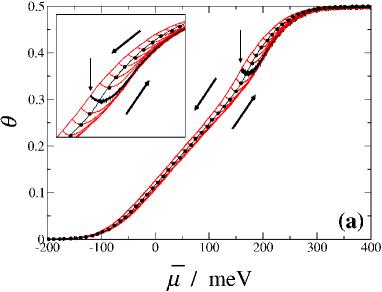
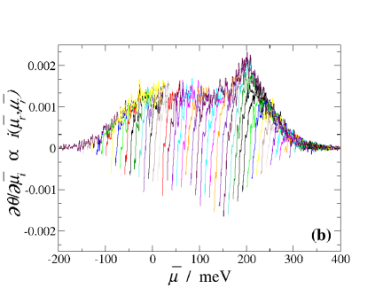
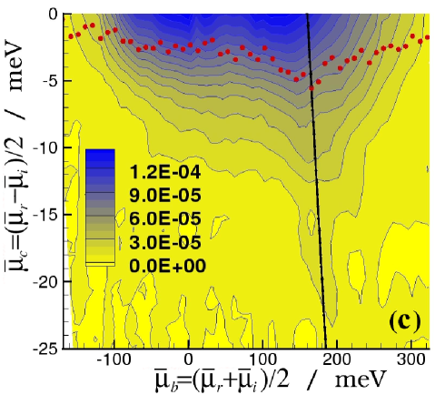
Figure 5: (a) Family of FORCs for our model of Br/Ag(100), corresponding to potential sweeps back and forth across the continuous phase transition between the disordered and $c(2\times 2)$ phases. The bold arrows show the directions of the potential sweeps, and the vertical arrow indicates $\bar{\mu}_{r}$ for one of the FORCs. The bold curve is the FORC whose minimum lies closest to the critical coverage (shown in more detail in the inset). The thin curve in the middle is the equilibrium isotherm. (b) Voltammetric currents corresponding to the FORCs in (a). (c) Contour plot of the FORC distribution $\rho$, corresponding to the FORCs in (a). The jagged curve of dots in the upper part of the diagram corresponds to the minima of the positive-going curves in (a). The area above the curve corresponds to desorption, and the area below it to adsorption. The slanted, straight line corresponds to the bold curve in (a). After Ref. HAMA07 .

The next step in extracting dynamical information from the FORCs or the corresponding currents is to calculate the FORC distribution,

$$\rho=-\frac{1}{2}\frac{\partial^{2}\Theta}{\partial\bar{\mu}_{r}\,\partial\bar{\mu}_{i}}=\frac{1}{2\gamma e({\rm d}\bar{\mu}_{i}/{\rm d}t)}\frac{\partial i(\bar{\mu}_{r},\bar{\mu}_{i})}{\partial\bar{\mu}_{r}}\;.$$ (18)

This is shown in Fig. 5(c) as a contour plot commonly known as a FORC diagram in terms of the more convenient variables $\bar{\mu}_{b}=(\bar{\mu}_{r}+\bar{\mu}_{i})/2$ and $\bar{\mu}_{c}=(\bar{\mu}_{r}-\bar{\mu}_{i})/2$ HAMA07 ; PIKE99 . Geometrically, $\rho$ is proportional to the vertical distance between adjacent current traces.

To our knowledge, the data for our model of Br/Ag(100) HAMA03 ; HAMA04 ; RIKV07 ; MITC00A ; MITC00C , which are shown in Fig. 5, are the first FORC predictions for a continuous phase transition. All three panels are significantly different from the corresponding data for a discontinuous transition, such as seen in underpotential deposition (UPD). In particular, the FORC distribution for a discontinuous transition contains a negative region, while this does not appear for continuous transitions. (See details in HAMA07 ; HAMA08 .) Closely related to this negative region is an extremum of the current density during the return scan FLET83 . EC-FORC analysis should be a useful and valuable method to distinguish between continuous and discontinuous phase transitions in experiments.

VII Conclusion

In this chapter we have presented some applications of the statistical-mechanics based computer-simulation methods of Molecular Dynamics and equilibrium and kinetic Monte Carlo simulations complemented by quantum-mechanical density functional theory calculations of interaction energies. These include both highly technologically-oriented applications to Lithium-battery technology, and basic-science investigations into adsorption on single-crystal electrodes. Our hope is that these examples and the list of references will encourage other workers in surface electrochemistry to take advantage of the recent spectacular advances in computational power and algorithmic sophistication to study ever-more detailed and accurate models of processes at solid-liquid interfaces.

References

- (1) D. M. Kolb, Surf. Sci. 500, 722 (2002).
- (2) T. Tansel and O. M. Magnussen, Phys. Rev. Lett. 96, 026101 (2006).
- (3) P. Vashishta, R. K. Kalia, and A. Nakano, J. Phys. Chem. B 110, 3727 (2006).
- (4) M. P. Allen and D. J. Tildesley, Computer Simulation of Liquids (Clarendon Press, Oxford, 1992).
- (5) J. M. Haile, Molecular Dynamics Simulation, Elementary Methods (John Wiley & Sons, New York, 1992).
- (6) D. C. Rapaport, The Art of Molecular Dynamics Simulation, 2nd ed. (Cambridge University Press, Cambridge, 2004).
- (7) A. F. Voter, Phys. Rev. Lett. 78, 3908 (1997).
- (8) A. F. Voter, J. Chem. Phys. 106, 4665 (1997).
- (9) J. Wang, R. Wolf, J. Caldwell, P. Kollman, and D. Case, J. Comp. Chem. 25, 1157 (2004).
- (10) J. C. Phillips, R. Braun, W. Wang, J. Gumbart, E. Tajkhorshid, E. Villa, C. Chipot, R. D. Skeel, L. Kalé, and K. Schulten, J. Comp. Chem. 26, 1781 (2005).
- (11) A. D. W. Humphrey and K. Schulten, J. Mol. Graphics 14, 33 (1996).
- (12) G. J. Martyna, D. J. Tobias, and M. L. Klein, J. Chem. Phys. 101, 4177 (1994).
- (13) S. E. Feller, Y. Zhang, R. W. Pastor, and B. R. Brooks, J. Chem. Phys. 103, 4613 (1995).
- (14) S. J. Mitchell, S. Wang, and P. A. Rikvold, Faraday Discussions 121, 53 (2002).
- (15) D. Huckaby and L. Blum, J. Chem. Phys. 92, 2646 (1990).
- (16) L. Blum and D. A. Huckaby, J. Electroanal. Chem. 375, 69 (1994).
- (17) L. Blum, D. A. Huckaby, and M. Legault, Electrochim. Acta 41, 2207 (1996).
- (18) M. Gamboa-Aldeco, P. Mrozek, C. K. Rhee, A. Wieckowski, P. A. Rikvold, and Q. Wang, Surf. Sci. Lett. 297, L135 (1993).
- (19) P. A. Rikvold, M. Gamboa-Aldeco, J. Zhang, M. Han, Q. Wang, H. L. Richards, and A. Wieckowski, Surf. Sci. 335, 389 (1995).
- (20) J. Zhang, Y.-S. Sung, P. A. Rikvold, and A. Wieckowski, J. Chem. Phys. 104, 5699 (1996).
- (21) T. L. Einstein, Langmuir 7, 2520 (1991).
- (22) P. Hyldgaard and T. L. Einstein, J. Cryst. Growth 275, e1637 (2005).
- (23) T. J. Stasevich, T. L. Einstein, and S. Stolbov, Phys. Rev. B 73, 115426 (2006).
- (24) P. A. Rikvold, J. B. Collins, G. D. Hansen, and J. D. Gunton, Surf. Sci. 203, 500 (1988).
- (25) J. B. Collins, P. Sacramento, P. A. Rikvold, and J. D. Gunton, Surf. Sci. 221, 277 (1989).
- (26) W. Schmickler, Interfacial Electrochemistry (Oxford Univ. Press, New York, 1996).
- (27) K. J. Vetter and J. W. Schultze, Ber. Bunsenges. Phys. Chem. 76, 920 (1972).
- (28) K. J. Vetter and J. W. Schultze, Ber. Bunsenges. Phys. Chem. 76, 927 (1972).
- (29) P. A. Rikvold, Th. Wandlowski, I. Abou Hamad, S. J. Mitchell, and G. Brown, Electrochim. Acta 52, 1932 (2007).
- (30) I. Abou Hamad, S. J. Mitchell, Th. Wandlowski, P. A. Rikvold, and G. Brown, Electrochim. Acta 50, 5518 (2005).
- (31) M. T. M. Koper, J. Electroanal. Chem. 450, 189 (1998).
- (32) J. N. Glosli and M. R. Philpott, in Microscopic Models of Electrode-Electrolyte Interfaces; Electrochem. Soc. Conf. Proc. Ser. 93-5, edited by J. W. Halley and L. Blum (The Electrochemical Society, Pennington, 1993), pp. 80–89.
- (33) J. N. Glosli and M. R. Philpott, in Microscopic Models of Electrode-Electrolyte Interfaces; Electrochem. Soc. Conf. Proc. Ser. 93-5, edited by J. W. Halley and L. Blum (The Electrochemical Society, Pennington, 1993), pp. 90–105.
- (34) L. Blum, Adv. Chem. Phys. 78, 171 (1990).
- (35) A. Ignaczak, J. A. N. F. Gomes, and S. Romanowski, J. Electroanal. Chem. 450, 175 (1998).
- (36) G. Brown, P. A. Rikvold, S. J. Mitchell, and M. A. Novotny, in Interfacial Electrochemistry: Theory, Experiment, and Application, edited by A. Wieckowski (Marcel Dekker, New York, 1999), pp. 47–61.
- (37) S. J. Mitchell, G. Brown, and P. A. Rikvold, J. Electroanal. Chem. 493, 68 (2000).
- (38) S. J. Mitchell, G. Brown, and P. A. Rikvold, Surf. Sci. 471, 125 (2001).
- (39) I. Abou Hamad, Th. Wandlowski, G. Brown, and P. A. Rikvold, J. Electroanal. Chem. 554-555, 211 (2003).
- (40) P. Hohenberg and W. Kohn, Phys. Rev. 136, B864 (1964).
- (41) W. Kohn and L. J. Sham, Phys. Rev. 140, A1133 (1965).
- (42) I. Abou Hamad, P. A. Rikvold, and G. Brown, Surf. Sci. 572, L355 (2004).
- (43) G. Kresse and J. Hafner, Phys. Rev. B 47, 558 (1993).
- (44) G. Kresse and J. Furthmüller, Phys. Rev. B 54, 11169 (1996).
- (45) G. Kresse and J. Furthmüller, Comput. Mater. Sci. 6, 15 (1996).
- (46) J. P. Perdew and Y. Wang, Phys. Rev. B 45, 13244 (1992).
- (47) J. P. Perdew, J. A. Chevary, S. A. Vosko, K. A. Jackson, M. R. Pederson, D. J. Singh, and C. Fiolhais, Phys. Rev. B 46, 6671 (1992).
- (48) D. Vanderbilt, Phys. Rev. B 41, 7892 (1990).
- (49) H. J. Monkhorst and J. D. Pack, Phys. Rev. B 13, 5188 (1976).
- (50) S. J. Mitchell and M. T. M. Koper, Surf. Sci. 563, 169 (2004).
- (51) W. Kohn and K.-H. Lau, Solid State Commun. 18, 553 (1976).
- (52) T. Juwono and P. A. Rikvold, unpublished.
- (53) D. P. Landau and K. Binder, A Guide to Monte Carlo Simulations in Statistical Physics, 2nd Ed. (Cambridge University Press, Cambridge, 2005).
- (54) S. Wang, S. J. Mitchell, and P. A. Rikvold, Comp. Mater. Sci. 29, 145 (2004).
- (55) P. A. Rikvold and M. Kolesik, J. Phys. A 35, L117 (2002).
- (56) P. A. Rikvold and M. Kolesik, Phys. Rev. E 66, 066116 (2002).
- (57) P. A. Rikvold and M. Kolesik, Phys. Rev. E 67, 066113 (2003).
- (58) K. Park, P. A. Rikvold, G. M. Buendía, and M. A. Novotny, Phys. Rev. Lett. 92, 015701 (2004).
- (59) G. M. Buendía, P. A. Rikvold, K. Park, and M. A. Novotny, J. Chem. Phys. 121, 4193 (2004).
- (60) G. M. Buendía, P. A. Rikvold, and M. Kolesik, Phys. Rev. B 73, 045437 (2006).
- (61) G. M. Buendía, P. A. Rikvold, and M. Kolesik, J. Mol. Struct.: THEOCHEM 769, 207 (2006).
- (62) G. M. Buendía, P. A. Rikvold, M. Kolesik, K. Park, and M. A. Novotny, Phys. Rev. B 76, 045422 (2007).
- (63) S. Wang, Y. Cao, and P. A. Rikvold, Phys. Rev. B 70, 205410 (2004).
- (64) A. Ignaczak and J. A. N. F. Gomes, J. Electroanal. Chem. 420, 71 (1997).
- (65) S. Wang and P. A. Rikvold, Phys. Rev. B 65, 155406 (2002).
- (66) A. Bogicevic, S. Ovesson, P. Hyldgaard, B. I. Lundquist, H. Brune, and D. R. Jennison, Phys. Rev. Lett. 85, 1910 (2000).
- (67) H. C. Kang and W. H. Weinberg, J. Chem. Phys. 90, 2824 (1989).
- (68) K. A. Fichthorn and W. H. Weinberg, J. Chem. Phys. 95, 1090 (1991).
- (69) A. B. Bortz, M. H. Kalos, and J. L. Lebowitz, J. Comput. Phys. 17, 10 (1975).
- (70) G. H. Gilmer, J. Crystal Growth 35, 15 (1976).
- (71) S. Frank and P. A. Rikvold, Surf. Sci. 600, 2470 (2006).
- (72) R. J. Gelten, A. P. J. Jansen, R. A. van Santen, J. J. Lukkien, J. P. L. Segers, and P. A. J. Hilbers, J. Chem. Phys. 108, 5921 (1998).
- (73) J. J. Lukkien, J. P. L. Segers, P. A. J. Hilbers, R. J. Gelten, and A. P. J. Jansen, Phys. Rev. E 58, 2598 (1998).
- (74) M. T. M. Koper, A. P. J. Jansen, R. A. van Santen, J. J. Lukkien, and P. A. J. Hilbers, J. Chem. Phys. 109, 6051 (1998).
- (75) F. Nieto, C. Uebing, V. Pereyra, and R. J. Faccio, Vacuum 54, 119 (1999).
- (76) M. A. Novotny, in Annual Reviews of Computational Physics IX, edited by D. Stauffer (World Scientific, Singapore, 2001), pp. 153–210.
- (77) T. Ala-Nissila, R. Ferrando, and S. C. Ying, Adv. Phys. 51, 949 (2002).
- (78) I. D. Mayergoyz, IEEE Trans. Magn. 22, 603 (1986).
- (79) C. R. Pike, A. P. Roberts, and K. L. Verosub, J. Appl. Phys. 85, 6660 (1999).
- (80) C. R. Pike, Phys. Rev. B 68, 104424 (2003).
- (81) D. T. Robb, M. A. Novotny, and P. A. Rikvold, J. Appl. Phys. 97, 10E510 (2005).
- (82) I. Abou Hamad, D. T. Robb, and P. A. Rikvold, J. Electroanal. Chem. 607, 61 (2007).
- (83) I. Abou Hamad, D. T. Robb, M A. Novotny, and P. A. Rikvold, ECS Transactions, in press (2008).
- (84) S. Fletcher, C. S. Halliday, D. Gates, M. Westcott, T. Lwin, and G. Nelson, J. Electroanal. Chem. 159, 267 (1983).