Effects on the two-point correlation function from the coupling of quintessence to dark matter

Abstract

We investigate the effects of the nonminimal coupling between the scalar field dark energy (quintessence) and the dark matter on the two-point correlation function. It is well known that this coupling shifts the turnover scale as well as suppresses the amplitude of the matter power spectrum. However, these effects are too small to be observed when we limit the coupling strength to be consistent with observations. Since the coupling of quintessence to baryons is strongly constrained, species dependent coupling may arise. This results in a baryon bias that is different from unity. Thus, we look over the correlation function in this coupled model. We are able to observe the enhancement of the baryon acoustic oscillation (BAO) peak due to the increasing bias factor of baryon from this species dependent coupling. In order to avoid the damping effect of the BAO signature in the matter power spectrum due to nonlinear clustering, we consider the coupling effect on the BAO bump in the linear regime. This provides an alternative method to constrain the coupling of dark energy to dark matter.

¹Institute of Physics, Academia Sinica, Taipei, Taiwan 11529, R.O.C.

²Leung Center for Cosmology and Particle Astrophysics, National Taiwan University, Taipei, Taiwan 10617, R.O.C.

³Department of Physics, Tamkang University, Tamsui, Taipei County, Taiwan 251, R.O.C.

⁴Institute of Astronomy and Astrophysics, Academia Sinica, Taipei, Taiwan 11529, R.O.C.

Due to the strong constraint on the coupling of the scalar field dark energy (quintessence) to baryons from the local gravity, we investigate the effect of the species dependent coupling [1, 2] by considering a model in which the quintessence $Q$ is only coupled to the cold dark matter (CDM). We assume a Yukawa-type coupling, $m_{c}=e^{n{c}Q}m^{*}_{c}$, where $m_{c}^{*}$ is the bare mass of the CDM [3, 4]. This specific choice of coupling requires that the present value of the scalar field vanishes in order to satisfy $m_{c}=m_{c}^{*}$ at present. Then we are able to write the general action including this interaction as

$$S=-\int d^{4}x\sqrt{-g}\Biggl{\{}\frac{\bar{M}^{2}}{2}\Bigl{[}-R+\partial^{\mu}Q\partial_{\mu}Q\Bigr{]}+V(Q)-{\cal L}_{c}-{\cal L}_{r}-{\cal L}_{b}\Biggr{\}},$$ (1)

where $\bar{M}=1/\sqrt{8\pi G}$ is the reduced Planck mass, $V(Q)$ is the potential of $Q$, and ${\cal L}_{r}$ and ${\cal L}_{i}=-m_{i}\delta(\vec{x}-\vec{x}_{i}(t))\sqrt{g_{\mu\nu}\dot{x}_{i}^{\mu}\dot{x}_{i}^{\nu}/g}$ ($i=c,b$) denote the Lagrangian of radiation, CDM, and baryons respectively. We adopt $V(Q)=V_{0}\exp(\lambda Q^{2}/2)$ with $\lambda=5$ in the following [4, 5]. However, the main conclusions are independent of the form of the scalar field potential (see below). Due to the coupling, the scalings of the CDM and the quintessence energy densities are changed respectively to [5]

$$\rho_{c}(a) = \rho_{c}^{0}a^{-3+\epsilon}\,\hskip 7.22743pt{\rm where}\hskip 7.22743pt\epsilon\ln(a)=n_{c}\Bigl{[}Q(a)-Q(1)\Bigr{]}\,,$$ (2)

$$\rho_{Q}^{\prime} = -3{\cal H}(1+\omega_{Q}^{\rm{eff}})\rho_{Q}\,\,\hskip 7.22743pt{\rm where}\hskip 7.22743pt\omega_{Q}^{\rm{eff}}=\omega_{Q}+\frac{n_{c}}{{\cal H}}\frac{\rho_{c}}{\rho_{Q}}Q^{\prime}\,,$$ (3)

where ${\cal H}\equiv(da/d\eta)/a$, $\omega_{Q}$ is the equation of state (eos) of the quintessential dark energy (DE), $\rho_{c}^{0}$ denotes the present value of the CDM energy density, the present value of scale factor $a_{0}=1$, and primes mean the differentiation with respect to the conformal time $\eta$. Generally, the sign of $\epsilon$ depends on both the model and the form of the coupling. The linear perturbation equations for the CDM and the scalar field $Q$ in the synchronous gauge are [6]

$$\delta_{c}^{\prime} = -\theta_{c}-\frac{1}{2}h^{\prime}+n_{c}\delta Q^{\prime}\,,$$ (4)

$$\theta_{c}^{\prime} = -{\cal H}\theta_{c}+n_{c}\Bigl{(}k^{2}\delta Q-Q^{\prime}\theta_{c}\Bigr{)}\,,$$ (5)

$$\delta Q^{\prime\prime} + 2{\cal H}\delta Q^{\prime}+k^{2}\delta Q+\frac{a^{2}}{\bar{M}^{2}}\frac{\partial^{2}V}{\partial Q^{2}}\delta Q=-\frac{1}{2}h^{\prime}Q^{\prime}-\frac{a^{2}}{\bar{M}^{2}}\rho_{c}n_{c}\delta_{c}\,,$$ (6)

where $k$ is the wave-number, $h$ is the metric perturbation, $\delta_{c}=\delta\rho_{c}/\rho_{c}$, and $\theta_{c}$ is the gradient of the CDM velocity flow. Also from the perturbed Einstein equations, we obtain

$$\frac{1}{2}(h^{\prime\prime}+{\cal H}h^{\prime})=-\frac{a^{2}}{2\bar{M}^{2}}\Bigl{[}2\delta\rho_{r}+\delta\rho_{c}+(1+3c_{b}^{2})\delta\rho_{b}+\frac{4\bar{M}^{2}}{a^{2}}Q^{\prime}\delta Q^{\prime}-2\frac{\partial V}{\partial Q}\delta Q\Bigr{]}\,,$$ (7)

where $c_{b}$ is the sound speed of baryons. Note that we will adopt the adiabatic initial conditions and thus $k^{2}\delta_{c}$ term is absent in Eq. (5).

The coupling strength $n_{c}$ is commonly constrained through the comparison with the observed cosmic microwave background anisotropy and matter power spectrum. In Ref. [5], we found $n_{c}\leq 0.01$. Even though the actual value of the upper limit depends on the form of the quintessence potential and that of the coupling, the obtained limits for other potentials and couplings are of the same order as shown in Ref. [7]. Furthermore, Eqs. (4) and (5), which describe the evolutions of the CDM density and velocity field respectively, imply that the influence of the quintessence field are dwarfed by the background evolution, ${\cal H}$. Thus, as long as we have the late-time dominated quintessence model, the evolution behaviors of Eqs. (4) and (5) are quite similar and almost independent of the form of potential. However, we have also checked the early dark energy model, for example, with the potential given by $V(Q)=V_{0}\cosh(\lambda Q)$, in which the dark energy component is not negligible at early times [8]. In this model, ${\cal H}$ is quite different from the quintessence model with the exponential potential and produce a quite different behavior of $\delta_{c}$. Here we will concentrate on the late quintessence model.

Even though we use the full set of the above equations for our calibration, we investigate the effects of coupling on the matter power spectrum with some approximation in what follows. It is well known that averaging out the small and oscillatory $\delta Q^{\prime\prime}$ and $\delta Q^{\prime}$ is a good approximation for all scales [9]. From this fact, we obtain the approximate expression of $\delta Q$ from Eq. (6)

$$\delta Q\simeq-\frac{\frac{a^{2}}{\bar{M}^{2}}n_{c}\rho_{c}\delta_{c}+\frac{1}{2}Q^{\prime}h^{\prime}}{\frac{a^{2}}{\bar{M}^{2}}m_{Q}^{2}+k^{2}}\,,$$ (8)

where $m_{Q}^{2}\equiv\partial^{2}V/\partial Q^{2}$. We obtain the evolution equation of $\delta_{c}$ from Eqs. (4) and (5) by using Eq. (8),

$$\delta_{c}^{\prime\prime}+{\cal H}\Bigl{[}1+n_{c}\sqrt{3(1+\omega_{Q})\Omega_{Q}}\,\Bigr{]}\delta_{c}^{\prime}-\frac{3}{2}{\cal H}^{2}\Omega_{c}\Bigl{(}1+2n_{c}^{2}\Bigr{)}\delta_{c}\simeq 0\,,$$ (9)

where $\Omega_{Q}$ is the quintessence energy density relative to the critical density and we use $Q^{\prime}={\cal H}\sqrt{3(1+\omega_{Q})\Omega_{Q}}$  [4]. The evolution of the linear perturbation of the baryon $\delta_{b}$ which is not coupled to the scalar field is the same as the above equation (9) except that now the coupling terms are absent:

$$\delta_{b}^{\prime\prime}+{\cal H}\delta_{b}^{\prime}-\frac{3}{2}{\cal H}^{2}\Omega_{c}\delta_{c}\simeq 0\,.$$ (10)

It is convenient to rewrite the above equations (9) and (10) in terms of $x=\ln a$ as

$$\frac{d^{2}\delta_{c}}{dx^{2}}+\Biggl{[}\frac{1}{2}-\frac{3}{2}\omega_{Q}\Omega_{Q}+n_{c}\sqrt{3(1+\omega_{Q})\Omega_{Q}}\,\Biggr{]}\frac{d\delta_{c}}{dx}$$

$$-\frac{3}{2}(1+2n_{c}^{2})\Omega_{c}\delta_{c}\simeq 0\,,$$ (11)

$$\frac{d^{2}\delta_{b}}{dx^{2}}+\Biggl{(}\frac{1}{2}-\frac{3}{2}\omega_{Q}\Omega_{Q}\,\Biggr{)}\frac{d\delta_{b}}{dx}-\frac{3}{2}\frac{1}{b}\Omega_{c}\delta_{b}\simeq 0\,,$$ (12)

$${\rm where}\,\,\Omega_{Q}\simeq 1-\Omega_{c}\simeq\Biggl{[}1+\frac{\Omega_{c}^{0}}{\Omega_{Q}^{0}}\frac{e^{(-3+\epsilon)x}}{e^{-3\int_{0}^{x}[1+\omega_{Q}(x^{\prime})]dx^{\prime}}}\Biggr{]}^{-1}\,\,.$$ (13)

In Eq. (12), we define a baryon bias factor $b$ by $\delta_{b}\equiv b\delta_{c}$ with a small time variation (i.e. we ignore $db/dx$ and $d^{2}b/dx^{2}$ terms). If we further use the assumption that the linear growth of the CDM is given by $\delta_{c}\propto e^{mx}$ with $m<1$, then we will obtain the analytic form of $b$

$$b=\Biggl{[}1+2n_{c}^{2}-\frac{2n_{c}m\sqrt{3(1+\omega_{Q})\Omega_{Q}}}{3\Omega_{c}}\Biggr{]}^{-1}\,.$$ (14)

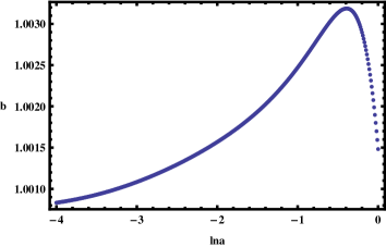
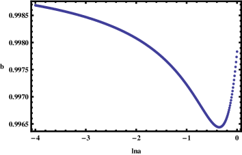
Figure 1: Evolutions of the baryon bias factor $b$ for the different couplings when $n_{c}=0.01$ (left panel) and $n_{c}=-0.01$ (right panel)

Here we use the ansatz for the coupling between CDM and DE as $e^{n_{c}Q}$. In our model, the scalar field evolves from $-5$ to $0$ during $10^{-10}\leq a\leq 1$. We put a limit on the magnitude of the coupling constant $|n_{c}|\leq 0.01$, where the choice of the sign of $n_{c}$ is still arbitrary. The effective mass of the CDM varies at most around $5$ %. $m_{c}$ (equally, $\rho_{c}$) increases (decreases) as it evolves to the present for the positive (negative) $n_{c}$. Thus, the evolutions of the background quantities are slightly changed dependent on the sign of $n_{c}$. The effect of the coupling on the $b$ also depends on the sign of $n_{c}$ as given in Eq. (14), which is used to estimate $b$ as shown in Fig. 1. In the left panel of Fig. 1, we show the evolution of $b$ when $n_{c}=+0.01$. For the positive $n_{c}$, the last term in Eq. (14) is negative and its magnitude is bigger than $2n_{c}^{2}$ for the given model. Thus, $b\geq 1$. The evolution of $b$ for $n_{c}=-0.01$ is depicted in the right panel of Fig. 1. In this case, the last term in Eq. (14) is positive and $b$ is always smaller than $1$. Thus, we are able to constrain not only the magnitude but also the form of the coupling between CDM and DE from accurate observations of the baryon power spectrum. A similar but slightly different conclusion was drawn in Ref. [10]; however, their conclusion is only true for the tracking region solutions.

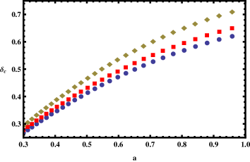
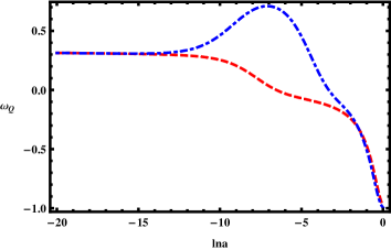
Figure 2: a) Evolutions of $\delta_{c}$ in the $\Lambda$CDM, QCDM, and cQCDM models (from top to bottom). b) Evolutions of the equation of state of Q field, $\omega_{Q}$, for the coupled and noncoupled cases (from top to bottom).

First, we study the CDM density fluctuation $\delta_{c}$ given in Eq. (11) for different cases. We denote respectively the cosmological model including CDM component with the cosmological constant as $\Lambda$CDM, with the non-coupled Q field ($n_{c}=0$) as QCDM, and with the coupled Q field as cQCDM. We also denote $\delta_{c}$ for each model as $\delta_{c}^{\Lambda CDM}$, $\delta_{c}^{QCDM}$, and $\delta_{c}^{cQCDM}$. $\delta_{c}^{QCDM}$ has the same evolution equations as those of the $\Lambda$CDM model except the difference in $\Omega_{Q}$ given in Eq. (13). $\omega_{Q}$ in the QCDM model changes from $1/3$ in the radiation-dominated epoch (the so-called “early tracking region”) to around $-1$ at present. Thus, $\omega_{Q}>\omega_{\Lambda}=-1$ during the entire epoch. This causes the suppression of $\delta_{c}$ in QCDM model compared to $\Lambda$CDM model when we use the same present values of the cosmological parameters. We illustrate this in the left panel of Fig. 2. The diamond and the rectangular points correspond to $\delta_{c}^{\Lambda CDM}$ and $\delta_{c}^{QCDM}$, respectively. We also compare $\delta_{c}^{QCDM}$ and $\delta_{c}^{cQCDM}$. When the CDM is coupled to Q field, the scaling of $\rho_{m}$ is changed as given in Eq. (2). Also $\omega_{Q}$ is increased during the matter-domination epoch in the cQCDM model as shown in the right panel of Fig. 2. The dot-dashed and the dashed lines depict $\omega_{Q}$ when $n_{c}=0.01$ and $0$, respectively. Thus, this causes slightly further suppression of $\delta_{c}$ in the cQCDM model. However, if we want to compare $\delta_{c}^{cQCDM}$ with $\delta_{c}^{QCDM}$ at the relevant sub-horizon scale, then we should constrain their evolutions at late times $a\geq 0.1$ (equally, $x\geq-2.3$). But then $\omega_{Q}$s of the two models are almost identical as shown in the right panel of Fig. 2 and the discrepancy between $\delta_{c}^{cQCDM}$ and $\delta_{c}^{QCDM}$ becomes negligible. If we use the definition of the baryon bias factor $b=\frac{\delta_{b}}{\delta_{c}}$, then we would obtain that $b_{cQCDM}>b_{QCDM}\simeq b_{\Lambda CDM}\simeq 1$ for the same present values of the cosmological parameters.

Now we consider the previously mentioned differences in the two-point correlation functions in different models. Instead of using the above approximations, we will run the numerical evolution of the full system of equations. The coupling of the quintessence to the dark matter modifies both the turnover scale and the amplitude of the matter power spectrum. However, the shift in the turnover scale and the suppression in the amplitude of the matter power spectrum (defined by $P(k)=\langle|\delta_{k}|^{2}\rangle\equiv(2\pi^{2})/k^{3}\Delta^{2}(k)$) due to this coupling are too small when we limit the coupling strength to be consistent with observations. Thus, this gives us the motivation to probe the coupling effects on the baryon acoustic peak in the correlation function, $\xi(s)=\int\Delta^{2}(k)J_{0}(ks)d\ln k$, where $J_{0}$ is the spherical Bessel function. In order to avoid the damping effect of the BAO signature in the matter power spectrum due to nonlinear clustering, we put the limitation of $k\leq 0.2h\,{\rm Mpc}^{-1}$ in our correlation function calculation. We show the correlation function times the comoving separation square ($s^{2}$) in Fig. 3. The solid, dashed, and dotted lines correspond to the $\Lambda$CDM, QCDM, and cQCDM models, respectively. The cosmological parameters that we use in this figure are $H_{0}=71\,{\rm km/sec/Mpc}$, $\Omega_{b}=0.047$, $\Omega_{c}=0.211$, $\Omega_{Q}=0.742$, and the galaxy bias factor $b_{gal}=1.9$. We also normalize the matter power spectrum to $\sigma_{8}=0.788$ to be consistent with the WMAP and the Luminous Red Galaxies (LRG) observations [11]. Note that the influence of DE on the present value of $\sigma_{8}=\sqrt{\int_{0}^{k}W^{2}(kR_{8})\Delta^{2}(k)d\ln k}$, where $W(x)=3(\sin x/x^{3}-\cos x/x^{2})$ is the Fourier transform of a top-hat window function and $R_{8}=8h^{-1}{\rm Mpc}$, is well studied [12, 13, 14, 15].

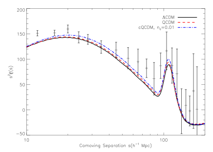
Figure 3: Matter correlation functions for $\Lambda$CDM, QCDM, and cQCDM models.

In Fig. 3, we are able to clearly see the differences of the correlation functions for the different models. The first peak in the correlation function corresponds to the turnover scale which is related to the scale factor $a_{eq}\sim 1/3500$ when the radiation and the matter densities are equal. The $\Lambda$CDM and QCDM models have the same $a_{eq}$ for the same set of cosmological parameters while their comoving distances of the matter and radiation equality, $s_{eq}$, are $19.17$ ${\rm Mpc}/h$ and $19.60$ ${\rm Mpc}/h$, respectively. The discrepancy comes from the fact that the comoving distance to the $a_{eq}$ is $\int_{0}^{t_{eq}}\frac{dt^{\prime}}{a(t^{\prime})}=\int_{z_{eq}}^{\infty}\frac{dz^{\prime}}{H(z^{\prime})}$ and the two models have slightly different $H(z)$. Also, the location of $s_{eq}$ in the cQCDM model is different from that in the QCDM model due to the change in the scaling of the CDM density. In our model, $\epsilon>0$ and it causes the delay of the radiation and matter equality epoch ($a_{eq}^{cQCDM}>a_{eq}^{QCDM}$). Thus, the comoving distance $s_{eq}$ is shifted to about $20.87$ ${\rm Mpc}/h$ in the coupled case.

We have already shown for the relevant $k$-modes, $\delta_{c}^{\Lambda CDM}>\delta_{c}^{QCDM}\simeq\delta_{c}^{cQCDM}$ for the same present values of the cosmological parameters. Thus, if we normalize the power spectra of the latter two models on cluster scales $\sigma_{8}$, they acquire a larger amplitude of primordial fluctuations compared to the $\Lambda$CDM model. The BAO bump in the correlation function of both QCDM and cQCDM models are larger than that of the $\Lambda$CDM model. However, the reason for the enhancements of the BAO bumps in both models are different. The enhancement in the QCDM model compared to the $\Lambda$CDM one is due to the choice of the larger amplitude of primordial fluctuations. The enhancement in the cQCDM model is due to the coupling between Q and CDM. We observe this effect in Fig. 3. If we compare the BAO peak of cQCDM with that of $\Lambda$CDM or QCDM, then we observe that it is enhanced in the cQCDM model. This is consistent with our early explanation that the baryon bias factor in the cQCDM model is enhanced as given in Eq. (14). The overall amplitudes of all three models in Fig. 3 are smaller than those given in Ref. [16]. This is due to the different choices of the galaxy bias factor. We use the LRG galaxy bias factor $b_{gal}=1.9$ [11] whereas the authors in Ref. [16] claim that they use the scale dependence bias factor which is however not given therein. However, both the shapes of the correlation functions and the amplitudes of the BAO bumps of the QCDM and cQCDM models fit to the data points better than the $\Lambda$CDM model. As we mentioned above, if we choose a negative $n_{c}$, then the amplitude of the BAO bump in the cQCDM model is decreased due to anti-biasing of baryons with $b<1$. This effect mimics the nonlinear effect [17]. It will suppress the amplitude and shift the location of the BAO bump, and thus making harder for us to fit the data. However, we limit the calculation in the linear regime and this effect is irrelevant for our consideration. In the Figure 3 of Ref. [16], it is claimed that $\Omega_{c}h^{2}=0.13$ shows the better fit to the data compared to the case using $\Omega_{c}h^{2}=0.12$. However, the amplitude of the BAO bump with $\Omega_{c}h^{2}=0.13$ shows the bigger discrepancy with the data than that with $\Omega_{c}h^{2}=0.12$. We are able to give a better direction for fitting both the shape and the amplitude of the correlation function in the QCDM and cQCDM models. We have done a simple $\chi^{2}$ analysis and found that the $\chi^{2}$ values are $21.6$, $21.7$, and $23.4$ for the $\Lambda$CDM, QCDM, and cQCDM models, respectively. Although the improvement has low statistical significance, the species-dependent coupling effects to the correlation function in the coupled quintessence model may be potentially important and are being further studied. Note that there is a slight shift in the location of the BAO peak in the QCDM model. This is due to the change in $H(z)$ in the QCDM model compared to the $\Lambda$CDM model. This affects the sound horizon that is given by $l_{s}=\int_{z_{dec}}^{\infty}\frac{c_{s}}{H(z)}dz$, where the sound speed of the baryon-photon fluid $c_{s}=1/\sqrt{3(1+3\rho_{b}/4\rho_{r})}$ is the same for every model. Hence, for each model we have a different $H(z)$ and $l_{s}$ will vary. However, the difference is quite small.

References

- [1] T. Damour and K. Nordtvedt, Phys. Rev. Lett. 70, 2217 (1993); T. Damour and K. Nordtvedt, Phys. Rev. D 48, 3436 (1993).
- [2] T. Damour and A. M. Polyakov, Nucl. Phys. B 423, 532 (1994) [arXiv:hep-th/9401069]; Gen. Rel. Grav 26, 1171 (1994) [arXiv:gr-qc/9411069].
- [3] G. R. Farrar and P. J. E. Peebles, Astrophys. J. 604, 1 (2004) [arXiv:astro-ph/0307316].
- [4] S. Lee, K. A. Olive, and M. Pospelov, Phys. Rev. D 70, 083503 (2004) [arXiv:astro-ph/0406039].
- [5] S. Lee, G.-C. Liu, and K.-W. Ng, Phys. Rev. D 73, 083516 (2006) [arXiv:astro-ph/0601333].
- [6] L. Amendola, Phys. Rev. D 69, 103524 (2004) [arXiv:astro-ph/0311175].
- [7] R. Bean, E. E. Flanagan, I. Laszlo, and M. Trodden, Phys. Rev. D 78, 123514 (2008) [arXiv:0808.1105]. ; G. L. Vacca, J. R. Kristiansen, L. P. L. Colombo, R. Mainini, and S. A. Bonometto, JCAP 0904:007 (2009) [arXiv:0902.2711].
- [8] W. Lee and K.-W. Ng, Phys. Rev. D 67, 107302 (2003) [arXiv:astro-ph/0209093]. ; R. R. Caldwell, M. Doran, C. M. Mueller, G. Schaefer, and C. Wetterich, Astrophys. J. 591, L75 (2003) [arXiv:astro-ph/0302505].
- [9] T. Koivisto, Phys. Rev. D 72, 043516 (2005) [arXiv:astro-ph/0504571].
- [10] L. Amendola and D. Tocchini-Valentini, Phys. Rev. D 66, 043528 (2002) [arXiv:astro-ph/0111535].
- [11] M. Tegmark et al. , Phys. Rev. D 74, 123507 (2006) [arXiv:astro-ph/0608632].
- [12] L. Wang and P. J. Steinhardt, Astrophys. J. 508, 483 (1998) [arXiv:astro-ph/9804015].
- [13] M. Doran, J.-M. Schwindt, and C. Wetterich, Phys. Rev. D 64, 123520 (2001) [arXiv:astro-ph/0107525].
- [14] M. Bartelmann, F. Perrotta, and C. Baccigalupi, Astron. Astrophys. 396, 21 (2002) [arXiv:astro-ph/0206507].
- [15] M. Kunz, P.-S. Corasaniti, D. Parkinson, and E. J. Copeland, Phys. Rev. D 70, 041301 (2004) [arXiv:astro-ph/0307346].
- [16] D. J. Eisenstein et al. , Astrophys. J. 633, 560 (2005) [arXiv:astro-ph/0501171].
- [17] M. Crocce and R. Scoccimarro, Phys. Rev. D 77, 023533 (2008) [arXiv:0704.2783].