Hyperuniformity in point patterns and two-phase random heterogeneous media
Abstract
Hyperuniform point patterns are characterized by vanishing infinite-wavelength density fluctuations and encompass all crystal structures, certain quasi-periodic systems, and special disordered point patterns [S. Torquato and F. H. Stillinger, Phys. Rev. E 68, 041113 (2003)]. This article generalizes the notion of hyperuniformity to include also two-phase random heterogeneous media. Hyperuniform random media do not possess infinite-wavelength volume fraction fluctuations, implying that the variance in the local volume fraction in an observation window decays faster than the reciprocal window volume as the window size increases. For microstructures of impenetrable and penetrable spheres, we derive an upper bound on the asymptotic coefficient governing local volume fraction fluctuations in terms of the corresponding quantity describing the variance in the local number density (i.e., number variance). Extensive calculations of the asymptotic number variance coefficients are performed for a number of disordered (e.g., quasiperiodic tilings, classical “stealth” disordered ground states, and certain determinantal point processes), quasicrystal, and ordered (e.g., Bravais and non-Bravais periodic systems) hyperuniform structures in various Euclidean space dimensions, and our results are consistent with a quantitative order metric characterizing the degree of hyperuniformity. We also present corresponding estimates for the asymptotic local volume fraction coefficients for several lattice families. Our results have interesting implications for a certain problem in number theory.
1 Introduction
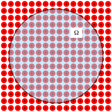
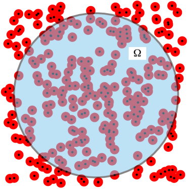
Characterizing the local fluctuations in a many-body system represents a fundamental problem in the physical and biological sciences [1]. Examples include the large-scale structure of the Universe [2], the structure and collective motion of grains in vibrated granular media [3], and the structure of living cells [4]. In each of these cases, one is interested in characterizing the variance in the local number of points of a general point pattern (henceforth known as the number variance), and this problem extends naturally to higher dimensions with applications to number theory [5, 6] and integrable quantum systems [7, 8, 9]. Of particular importance in this regard is the notion of hyperuniformity in a point pattern, in which the number variance in some local observation window grows more slowly than the mean as the size of the window increases [10]; such systems are also known as superhomogeneous [2]. Figure 1 shows typical periodic and nonperiodic point patterns along with the corresponding observation windows.
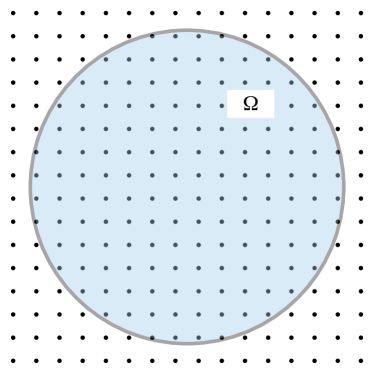
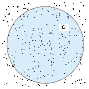
Torquato and Stillinger [10] have provided a rigorous characterization of both periodic and nonperiodic hyperuniform point patterns, which do not possess infinite-wavelength local density fluctuations. They have also computed the asymptotic number variance coefficients for a number of common lattices, including the square, triangular, FCC, and BCC crystal structures. Further examples of hyperuniform systems include all periodic point patterns, certain quasi-periodic systems, and special disordered point patterns. We remark that a mathematical (or Bravais) lattice is a system of points in Euclidean space with a set of minimal basis vectors such that any point in the lattice can be generated by taking integral linear combinations of the basis vectors. Other periodic structures can be formed by including more than one point in a fundamental cell, and we will occasionally refer to such structures as nonlattices. Unless otherwise noted, our usage of the term lattice will exclusively apply to Bravais lattices.
Here we generalize the notion of hyperuniformity to heterogeneous media, wherein one characterizes the local fluctuations in the volume fraction. A heterogeneous medium, also known in the mathematics literature as a random set, is a partition of -dimensional Euclidean space into disjoint regions (phases) with interfaces that are known only probabilistically. Throughout this paper we will consider two-phase heterogeneous media. Microstructural information for the system is contained in the indicator function for each phase , defined by:
| (3) |
Of particular importance is the so-called two-point probability function [11, 12, 13, 14], which is defined by:
| (4) |
where we have implicitly chosen some reference phase in the system. Note that since one can always construct a heterogeneous medium by “decorating” an appropriate point process (e.g., circumscription with hexagons or spheres; see Figure 1), characterizing the statistical properties of a heterogeneous medium represents a more general problem than the study of point patterns; namely, the latter systems are recovered as a special limit of the former. It is therefore intuitive that any physical application of point processes is also important for heterogeneous media. Applications of the hyperuniformity problem for such systems include scattering by heterogeneous media [15], transport through composites and porous media [16], the study of noise and granularity of photographic images [17, 18], identifying properties of organic coatings [19], and the fracture of composite materials [20]. In fact, it is generally true that any statistical description of the microstructure of a heterogeneous material provides nontrivial information about a wide variety of effective properties of that material in a homogenized sense [14].
The local volume fraction of a heterogeneous medium is defined as the fraction of the volume of an observation window covered by a particular phase (see Figure 1). For the remainder of this paper we consider spherical observation windows, but our results are easily extended to windows of arbitrary geometry [10]. Lu and Torquato [21] have studied the variance of , which they refer to as the coarseness after suitable scaling, and have shown in the homogeneous case that it is related to the two-point probability function according to:
| (5) |
where is the volume of a sphere of radius , is the so-called scaled intersection volume of two spheres of radius whose centers are separated by a distance (defined in more detail in Section 2), and is the fraction of space in the global medium occupied by the reference phase. For large windows, these authors showed that in non-hyperuniform media . Additionally, Quintanilla and Torquato [22] have determined the cumulative distribution functions of the local volume fraction for a number of low-dimensional periodic [23] and random [22] media; it is known that a central-limit result holds for sufficiently large observation windows [22]. We mention here that there is an analogous formula for the number variance of a point pattern:
| (6) |
where is the so-called total correlation function of the point process. The details behind these relations are provided in Sections 2 and 3, but it is clear from these remarks that the coarseness of a heterogeneous medium plays a similar role as the local density fluctuations in a point pattern. Figure 1 compares the hyperuniformity problem for point patterns and heterogeneous media in both the periodic and nonperiodic cases. Unlike the local number density, the local volume fraction approaches a fixed value on the global scale of the system, meaning that the coarseness must decay over large length scales. The analog of hyperuniformity in this instance will involve a decay in the local volume fraction fluctuations that is faster than the volume of the observation window; we quantify this behavior in Section 3 using the asymptotic scaling of the coarseness.
One important implication of this work is the development of a quantitative order metric characterizing the degree of order in a point pattern. From our experience with low-dimensional systems, it is physically intuitive that Bravais lattices are in some sense “more ordered” than nonlattice structures and quasicrystals, which in turn are seemingly more regular than strongly-correlated disordered point patterns. Furthermore, one also expects that weakly correlated systems are highly disordered. It is thus an open problem in statistical physics to quantify “randomness” in a many-body system with a simple metric that reflects this intuitive ordering. The observation that hyperuniform point patterns are characterized by a certain regularity in the distribution of points throughout suggests that quantitative measurements of the local number variance can provide one measure of order in point patterns, and we discuss the construction of such a metric in this work.
Section 2 reviews the basic notions of stochastic point processes, which are completely characterized by the set of -particle correlation functions, and hyperuniformity, which is defined completely by the two-particle information of the point process. Section 3 presents the corresponding results for two-phase heterogeneous media, whereby the fluctuations in the local volume fraction are related to two-point microstructural information of the phases. In general, if a heterogeneous medium can be generated from a stochastic point process, even lower-order microstructural information about the system will require a knowledge of the full -particle information of the underlying point process. However, we show in Section 4 that there is a convenient relation between fluctuations in the local number density and the corresponding fluctuations in the local volume fraction for microstructures of spherical inclusions, thereby providing a computationally accessible estimate of the local volume fraction variance. Section 5 presents explicit calculations of the asymptotic coefficients governing the local density fluctuations for a wide range of periodic and disordered point processes in low Euclidean dimensions, and these results translate into the aforementioned quantitative order metric characterizing the degree of (dis)order in a given arrangement of points. We extend these calculations in Section 6 to include the asymptotic properties of these terms for large Euclidean dimensions and also to provide information about the corresponding coefficients for the fluctuations in the local volume fraction. Extensive tables of asymptotic coefficients are provided for periodic and nonperiodic systems in Sections 5 and 6, and the reader who wishes to skip the mathematical details of the preceding sections is directed there. Our results have interesting implications for the minimzers of the Epstein zeta function, a fundamental problem that arises in number theory. Concluding remarks are given in Section 7.
2 Background and definitions
2.1 Point processes and -particle correlation functions
A stochastic point process in is defined as a mapping from a probability space to configurations of points in -dimensional Euclidean space . More precisely, let denote the set of configurations such that each configuration is a subset of that satisfies two regularity conditions: (i) there are no multiple points ( if ) and (ii) each bounded subset of must contain only a finite number of points of . We denote by the number of points within , , where is the ring of bounded Borel sets in . Thus, we always have for , but the possibility is not excluded. We note that there exists a minimal -algebra of subsets of that renders all of the functions measurable. Let be a probability space. Any measurable map is called a stochastic point process [11, 24]. Henceforth, we will simply call this map a point process. Note that this random setting is quite general; it incorporates cases in which the location of the points are deterministically known, such as a lattice.
A point process is completely specified by the countably infinite set of generic -particle probability density functions. The generic -particle probability density function, denoted by , is proportional to the probability density of finding particles in volume elements around the given positions , irrespective of the remaining particles. Specifically, if is the probability density for finding particles at positions , the generic -particle probability density is given by:
| (7) |
For a statistically homogeneous point process, the single-particle generic density function is:
| (8) |
where the limit in (8) defines the thermodynamic limit. This function is proportional to the probability density of finding a particle at , also known as the intensity of the point process. In general the normalization for is given by , or the number of ways of choosing an ordered subset of points from a population of size . For a translationally-invariant and completely uncorrelated point process for all .
We also introduce the -particle correlation functions , which are defined by:
| (9) |
Since for a completely uncorrelated point process, it follows that deviations of from unity provide a measure of the correlations between points in a point process. Of particular interest is the pair correlation function, which for a translationally-invariant point process of intensity can be written as:
| (10) |
Closely related to the pair correlation function is the total correlation function, denoted by ; it is derived from via the equation:
| (11) |
Since as () for translationally invariant systems without long-range order, it follows that in this limit, meaning that is generally an function, and its Fourier transform is well-defined.
It is common in statistical mechanics when passing to reciprocal space to consider the associated structure factor , which for a translationally invariant system is defined by:
| (12) |
where is the Fourier transform of the total correlation function, is the number density, and is the magnitude of the reciprocal variable to . We utilize the following definition of the Fourier transform:
| (13) |
where is the conventional Euclidean inner product of two real-valued vectors. When it is well-defined, the corresponding inverse Fourier transform is given by:
| (14) |
We remark that for radially-symmetric functions [i.e., ], the Fourier and inverse Fourier transforms may be written respectively as follows:
| (15) | |||||
| (16) |
2.2 Hyperuniform point processes
A hyperuniform point process has the property that the variance in the number of points in an observation window grows more slowly than the volume of that window. In the case of a spherical observation window, this definition implies that the local number variance grows more slowly than in dimensions, where is the radius of the observation window. Torquato and Stillinger [10] (see also [25, 26, 27] for related results) have provided an exact expression for the local number variance of a statistically homogeneous point process in a spherical observation window:
| (17) |
where is the radius of the observation window, is the volume of the window, and is the so-called scaled intersection volume. The latter quantity is geometrically defined as the volume of space occupied by the intersection of two spheres of radius separated by a distance normalized by the volume of a sphere . We remark that the average number of points in an observation window is for any statistically homogeneous point process.
The scaled intersection volume then has the support , the range , and the following alternative integral representation [24]:
| (18) |
where is a -dimensional constant given by
| (19) |
Torquato and Stillinger [24] found the following series representation of the scaled intersection volume for and for any :
| (20) |
where . For even dimensions, relation (20) is an infinite series, but for odd dimensions, the series truncates such that is a univariate polynomial of degree . It is convenient to introduce a dimensionless density , defined by:
| (21) |
where is a characteristic microscopic length scale of the system (e.g., the mean nearest-neighbor distance between points).
Using the expansion (20), the result in (17) admits the following asymptotic scaling [10]:
| (22) |
where denotes all terms of order less than . Explicit forms for the asymptotic coefficients and are given by:
| (23) | |||||
| (24) |
where with defined by (19); note that we have taken in the integrals, thereby rendering and independent of . These results are valid for all periodic point patterns (including lattices), quasicrystals that possess Bragg peaks, and disordered systems in which the pair correlation function decays to unity exponentially fast [10, 28]. Any such system with satisfies the requirements for hyperuniformity. The relation in (23) then implies that hyperuniform point patterns do not possess infinite-wavelength fluctuations in the local number density.
For disordered hyperuniform systems with a total correlation function that does not decay to zero exponentially fast, other dependencies of the number variance on may be observed. For example, it is known that if the total correlation function for large , then [8]. Such behavior occurs in maximally random jammed sphere packings [29] and noninteracting spin-polarized fermion ground states [8, 9]. More generally, for any reciprocal power law:
| (25) |
one can observe a number of different types of dependencies of the number variance on the window radius :
| (28) |
Note that it is not possible to construct a hyperuniform system for which since the number variance would then grow at least as fast as the volume of the observation window. It is also not possible to choose since the number variance cannot grow any slower than the surface area of the window [30, 10]. However, there are examples of point patterns that do not possess a surface area term in the number variance (i.e., ); these systems are known as hyposurficial point patterns [10].
Cases where the number variance grows faster than the window volume have been reported on the real line [31]. These non-hyperuniform systems exhibit what we describe as “super-Poissonian” behavior111Super-Poissonian point processes have also been called “sub-homogeneous” in the literature [31]. and are similar to thermodynamic critical points [10], where the structure factor diverges at the origin. Note that this behavior implies a scale-invariant structure. More generally, if a non-hyperuniform point pattern possesses a total correlation function:
| (29) |
then the number variance can exhibit the following asymptotic behaviors:
| (33) |
Note that the integrability requirement of the function implies that the number variance cannot grow any faster than the square of the window volume.
We remark that the problem of minimizing the number variance can be expressed in terms of finding the ground state of a pair interaction with compact support; namely, by invoking a volume-average interpretation of the number variance problem valid for a single realization of a point process, Torquato and Stillinger found [10]:
| (34) |
The asymptotic coefficient for a hyperuniform point pattern is then given by:
| (35) | |||||
| (36) |
These results imply that the asymptotic coefficient obtained in (24) involves an average over small-scale fluctuations in the number variance with length scale on the order of the mean separation between points [10].
There is another reformulation of the number variance problem [6, 10] in terms of the Epstein zeta function that is applicable for Bravais lattices. By recognizing that the number of points in an observation window for a Bravais lattice is a periodic function of the centroid of the window, one can establish the following expression for the asymptotic coefficient :
| (37) |
where is the volume of the fundamental cell and denotes a vector of the dual lattice. The Epstein zeta function for a lattice is given by [32]:
| (38) |
where is a vector of the lattice . It is clear from (37) that the dual of the lattice that minimizes the Epstein zeta function among all lattices will minimize the asymptotic coefficient for the number variance among lattices. We remark that minimization of the Epstein zeta function is equivalent to the problem of finding the classical ground state of an inverse power-law pair potential in dimension , which is completely monotonic. Torquato and Stillinger have provided certain duality relations [33] that establish rigorous upper bounds on the energies of such ground states and help to identify energy-minimizing lattices. It is known in two dimensions that the triangular lattice minimizes the Epstein zeta function [34, 35, 36, 37, 32] among all lattices; in three dimensions the FCC is at least a local minimum among lattices [38, 32], and for dimensions 4, 8, and 24 the densest known lattice packings are local minima [32]. However, it is almost certainly not true in higher dimensions that the minimizers of the Epstein zeta function are lattice structures since the densest packings are likely to be nonperiodic [24].
3 Local volume fraction fluctuations in two-phase heterogeneous media
3.1 Definition of the local volume fraction
We consider a two-phase heterogeneous random medium, which we now define to be a domain of space of volume that is composed of two regions: the phase 1 region of volume fraction and the phase 2 region of volume fraction [21]. In general for some realization of an underlying probability space. The statistical properties of each phase of the system are specified by the countably infinite set of -point probability functions , which are defined by [11, 12, 13, 14]:
| (39) |
where is the indicator function for phase . If the medium is statistically homogeneous, the volume fraction of phase is given by:
| (40) |
and this quantity is fixed on the global scale of the microstructure. However, the volume fraction fluctuates on a local scale determined by an observation window of arbitrary geometry as in the case of the local number density.
Specifically, we define the local volume fraction of phase according to:
| (41) |
where is the volume of the observation window and is the corresponding indicator function. Using this definition, the variance in the local volume fraction is given by:
| (42) |
which leads to the previously mentioned result:
| (43) |
where is the two-point probability function (for phase ) and is the scaled intersection volume. Note that:
| (44) |
therefore, we may express (43) in the form:
| (45) |
or, defining the autocovariance function :
| (46) |
We remark that as , and as in the absence of long-range order. Thus, for such systems it is true that , and its Fourier transform is well-defined; the same is true for .
3.2 Asymptotic behavior of the variance in the local volume fraction
For a homogeneous and isotropic system with a spherical observation window of radius , the result (46) implies:
| (47) |
where is the surface area of a -dimensional sphere and is the corresponding volume. For simplicity we drop the subscript on the local volume fraction with the disclaimer that our results apply for some specified reference phase in the heterogeneous system. Substitution of the expansion (20) for the scaled intersection volume into (47) implies:
| (48) | |||||
| (49) |
where:
| (50) | |||||
| (51) |
It is convenient as with the number variance to introduce a length scale , which can, for example, represent the diameter of a spherical inclusion in the heterogeneous medium. The results in (49)-(51) then take the forms:
| (52) | |||||
| (53) | |||||
| (54) |
The coefficients and in (53) and (54) control the asymptotic scaling of the fluctuations in the local volume fraction. We note that:
| (55) |
where is the Fourier transform of . It then follows that as for those systems such that:
| (56) |
This behavior is for random heterogeneous media the equivalent to hyperuniformity in the description of local number density fluctuations in stochastic point processes.
4 An estimate of using for microstructures of spherical inclusions
It is possible to derive a bound for the asymptotic coefficient governing fluctuations in the local volume fraction in terms of the corresponding coefficient for the local number density in the case of microstructures of spherical inclusions of radius . We first consider a system of impenetrable spheres and then generalize our results to the penetrable case. Note that this setting is quite general, incorporating lattice and ordered packing structures below the maximal packing fraction in addition to equilibrium and nonequilibrium distributions of hard spheres. To establish this connection, we first note that the series representation of for the matrix phase external to any inclusions is given in terms of the -particle correlation functions by [12, 13, 39, 21, 14]:
| (57) | |||||
where is a particle indicator function for an inclusion in phase . For the special case of inclusions of statistically homogeneous disjoint impenetrable spheres, (57) simplifies according to [21]:
| (58) |
where the last term is the convolution of the pair correlation function with the spherical intersection volume and is the volume fraction of inclusions. The result in (58) immediately implies that the autocovariance function for this system is:
| (59) |
and this equation is valid for either phase of the heterogeneous medium. It now follows from (53) that the coefficient is given by:
| (60) | |||||
| (61) | |||||
| (62) |
One can see that a hyperuniform point pattern derived from a system of impenetrable spheres generates a hyperuniform heterogeneous medium with respect to fluctuations in the local volume fraction. It is also clear that the leading-order asymptotic coefficient for the variance in the local volume fraction can be determined completely from the knowledge of , a more accessible quantity since it does not require the explicit calculation of the autocovariance function .
The calculation of is generally nontrivial, even for a medium of impenetrable spheres. Using an argument similar to the one for , one can establish the following exact relation between and :
| (63) |
there is no simple factorization of the -th moment of the convolution for which (63) simplifies. Therefore, the coefficient depends explicitly on the two-point information of the heterogeneous system. Nevertheless, one can establish a rigorous upper bound on in terms of . Toward this end, we first note that the local volume fraction of impenetrable spheres centered at with respect to a spherical observation window of radius is given by:
| (64) |
where is the center of the observation window and is the intersection volume between a sphere of radius and another sphere of radius given a separation between their centers. If the underlying probability distribution for the sphere centers is given by , then we immediately recover the result:
| (65) | |||||
| (66) |
where we have assumed statistical homogeneity and used the identity:
| (67) |
Using (64), we may also write:
| (68) | |||||
which implies:
| (69) |
where is the self-convolution of the intersection volume. The expression in (69) admits the following upper bound:
| (70) | |||||
| (71) | |||||
| (72) |
where . The result (70) uses the inequality where is the indicator function for a sphere of radius . Combining (66) and (72), we find:
| (73) | |||||
| (74) |
in the asymptotic limit we find :
| (75) |
Substituting the asymptotic expansions (22) and (52) into (75) gives an upper bound that is exact to according to (62). It is therefore true that:
| (76) |
The relation (76) is generally not an equality for a given heterogeneous system, and we provide a specific example in Section 6 where the strict inequality holds.
We remark that in situations where the microstructure of the heterogeneous medium consists of overlapping spheres, the variance in the local volume fraction is generally expected to be greater than the corresponding fluctuations for impenetrable inclusions at a fixed volume fraction [21, 22, 14]. This behavior arises since the excluded volume induced by an impenetrable shell formally induces a greater degree of uniformity in the underlying point process generated by the sphere centers, thereby reducing the variance in the local volume fraction. However, at a fixed reduced density , which is greater than the volume fraction of penetrable spheres, the general upper bound given in (75) (with the replacement ) will still hold. This claim is a direct result of the relation (64), the right-hand side of which becomes an upper bound for overlapping spheres at fixed . The remainder of the analysis leading to (75) therefore also works for this case with the exception that, for nonhyperuniform systems, the bound (76) becomes a bound on the leading-order coefficients and 222Careful replication of the analysis for hard spheres in the penetrable case actually shows ; the constant depends only on the reduced density and the volume fraction and plays no role for large windows.. For hyperuniform point patterns, the identity and the bound (75) immediately imply , even for microstructures of penetrable spheres, and we then retain the result (76) on and .
5 Low-dimensional local density fluctuations and order metrics
Although Torquato and Stillinger have provided some calculations of the asymptotic coefficients for certain periodic and disordered hyperuniform point patterns [10], an extensive classification of hyperuniform systems remains an active research area. Here we provide new calculations of the asymptotic coefficients for selected periodic and nonperiodic hyperuniform point patterns, including the Fibonacci chain, the so-called “tunneled crystals” introduced elsewhere by Torquato and Stillinger [40], a four-coordinate relative of the Kagomé lattice, the 4.8.8 Archimedean tiling of the plane, and certain classical disordered ground states in low Euclidean dimensions.
Our major results, including detailed tables of number variance coefficients for several hyperuniform point patterns, are collected in subsection 1. Since the current literature on hyperuniform point processes is disparate, we have provided details on several periodic, quasiperiodic, and nonperiodic hyperuniform point patterns, including processes introduced in this article and previously by other authors, in subsections 2 and 3. The information in these subsections is meant to supplement the key results of this article and should provide a brief and self-contained (though almost certainly not complete) overview of the field. Those readers interested only in the results may choose to skim this material.
5.1 Number variance coefficients for and
We collect in Tables 1-3 the asymptotic coefficients for several hyperuniform point patterns, and the results establish a quantitative order metric for point patterns, meaning that they measure the degree of regularity in the spatial distribution of the points. The details of accurately calculating for a given point process have been provided elsewhere [10]; described below are a number of pertinent results for characterizing the fluctuations in a hyperuniform point pattern.
The result (24) for the calculation of cannot in general be applied to periodic point patterns because such systems are not statistically homogeneous. Using the following radial form of the pair correlation function:
| (77) |
we find that the total correlation function is nonintegrable. However, one can obtain a convergent expression for using the following interpretation of (24) [10]:
| (78) |
which implies:
| (79) |
We note that to compare values of among different hyperuniform systems one should use the rescaled coefficient ; reference to (79) shows that this scaling eliminates the dependence on both the length scale and the reduced density . For and , (79) takes the forms:
| (80) | |||||
| (81) | |||||
| (82) |
The summations in (80)-(82) can be easily accomplished using the theta series for a periodic point pattern ; it is defined by:
| (83) |
where is the distance to the -th coordination shell and is the corresponding coordination number. This series can usually be generated from the simpler functions , and , which are defined by [41]:
| (84) | |||||
| (85) | |||||
| (86) |
These functions have the following intuitive interpretations: and assign points to the half-integer and integer positions, respectively, on the line, and assigns points to the even integers and removes points from the odd integers [41]. It thus follows that the theta series for the integer lattices and checkerboard lattices are given respectively by:
| (87) | |||||
| (88) |
The theta series for most well-known lattices have been tabulated analytically [41, 42]; they are directly related to the quadratic forms associated with the lattices.
With regard to nonperiodic systems, Torquato and Stillinger have developed a volume-average interpretation of the characterization of hyperuniform point patterns [10]; namely, the following relations hold for any single realization of a statistically homogeneous ergodic point process:
| (89) | |||
| (90) |
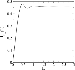
Note again that using the rescaled coefficient eliminates the dependence of the asymptotic coefficient on and according to (89); the length scale for the system is then determined by the reciprocal number density , and, making use of reduced units, it follows that once the problem has been solved for unit number density, it has been solved for all number densities. The result (89) captures small-scale fluctuations with respect to with a wavelength on the order of the mean separation between points; these fluctuations are superimposed on the large-scale variations with respect to [10]. These relations are useful in characterizing fluctuations in the local number density for disordered point patterns, where only limited information about the thermodynamic limit may be available. We remark, however, that any small-scale fluctuations in typically only appear for nearest-neighbor distances and rapidly vanish; as a result, one can obtain quite reliable results for given a realization of a point process with particles. Ensemble averaging improves these calculations, but large numbers of configurations are not always necessary to characterize a given point process. As few as configurations is empirically sufficient to determine using (89) and (90). Figure 2 demonstrates the dissipation in the small- fluctuations of .
| System | |||
|---|---|---|---|
| 0.08333 | 0.16667 | 1.00000 | |
| step+delta-function | 0.09375 | 0.18750 | 0.88889 |
| Fibonacci chain | 0.10055 | 0.20110 | 0.82878 |
| step-function | 0.12500 | 0.25 | 0.66667 |
| two-scale lattice | 0.14583 | 0.29167 | 0.57143 |
| lattice gas | 0.16667 | 0.33333 | 0.50000 |
| System | |||
|---|---|---|---|
| (triangular) | 0.12709 | 0.50835 | 1.00000 |
| 0.12910 | 0.51640 | 0.98443 | |
| disordered GS; | 0.13100 | 0.52400 | 0.97015 |
| disordered GS; | 0.13454 | 0.53816 | 0.94463 |
| honeycomb | 0.14176 | 0.56703 | 0.89652 |
| Kagomé | 0.14675 | 0.58699 | 0.86603 |
| octagonal tiling | 0.14892 | 0.59567 | 0.85341 |
| step+delta-function | 0.15005 | 0.60021 | 0.84698 |
| Penrose tiling | 0.15013 | 0.60052 | 0.84652 |
| 4-coordinate Kagomé relative | 0.15248 | 0.60990 | 0.83349 |
| disordered GS; | 0.15314 | 0.61254 | 0.82989 |
| tessellation | 0.17497 | 0.69987 | 0.72635 |
| step-function | 0.21221 | 0.84883 | 0.59889 |
| One-component plasma | 0.28210 | 1.12838 | 0.45051 |
| System | |||
|---|---|---|---|
| (BCC) | 0.15560 | 1.24476 | 1.00000 |
| (FCC) | 0.15569 | 1.24552 | 0.99942 |
| HCP | 0.15571 | 1.24569 | 0.99929 |
| 0.16115 | 1.28920 | 0.96556 | |
| disordered GS; | 0.16217 | 1.29737 | 0.95949 |
| (diamond) | 0.17737 | 1.41892 | 0.87726 |
| tunneled FCC | 0.17760 | 1.42080 | 0.87613 |
| würzite | 0.17773 | 1.42184 | 0.87549 |
| tunneled HCP | 0.17856 | 1.42845 | 0.87142 |
| damped-oscillating | 0.18105 | 1.44837 | 0.85943 |
| step+delta-function | 0.19086 | 1.52686 | 0.81526 |
| step-function | 0.28125 | 2.25000 | 0.55324 |
It is an open problem in the statistical physics of many-particle systems to construct simple scalar order metrics that quantify the degree of “randomness” in a point pattern. Such metrics are essential in defining the maximally random jammed state as discussed above and represent a fundamental way of characterizing point patterns in any dimension. One notices from the results in Tables 1-3 that lattice structures possess smaller asymptotic number variance coefficients compared to random point patterns; in other words, as a point pattern more closely resembles a Poisson point process, the number variance grows more quickly with the size of an observation window for large windows. This observation suggests that by normalizing the asymptotic coefficient by the corresponding result for the variance-minimizing structure, one can obtain a scalar quantity between 0 and 1 characterizing the extent of global order in the system. Specifically, we define the following order metric for a point pattern relative to the variance-minimizing structure for a given dimension:
| (91) |
We remark that the metric proposed in (91) is only one of many possible choices for characterizing order in a many-particle system. Since complete information about such a system is generally unavailable, one must almost always settle for reduced information about a system as contained in , which depends implicitly on the two-particle information of the point process. One advantageous property of (91) is that the choice of the reference structure is essentially not arbitrary since it is quantitatively well-defined by the variance-minimizing structure. It is possible (and in fact likely in higher dimensions) that such a structure will be degenerate, meaning that it will share the same two-point information with a number of other systems; however, this degeneracy does not affect the quantitative values of for all other structures once the minimum value of has been identified. This behavior is in contrast to other orientational and translational metrics [43, 44], which in three dimensions arbitrarily define the FCC lattice as the standard of perfect spatial ordering. Additionally, the fact that the order metric (91) classifies a quasicrystalline structure such as the Fibonacci chain or the Penrose tiling as being between perfect crystalline point patterns and correlated disordered systems is noteworthy because it is consistent with the notion that quasicrystals possess features of both of these types of systems. In other words, it is clear from Tables 1-3 that quasicrystals possess less order than any Bravais lattice, but there do exist “structured” disordered point patterns and periodic nonlattices with number variance coefficients of roughly the same magnitudes as quasicrystals. It is this observation which in part suggests the usefulness of hyperuniformity in understanding the degree of order within a point pattern; namely, we are able to identify a restricted set of point processes with an quantitative order metric that matches our intuition of the relative extent of (dis)order within a system.
5.2 Known hyperuniform systems
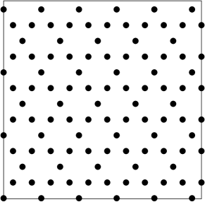
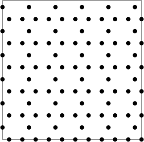
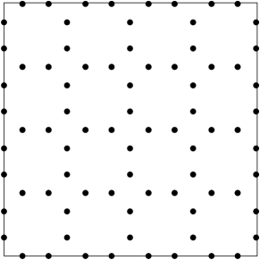
On account of its long-range order, any periodic point pattern is hyperuniform [10]. Although such systems are not strictly statistically homogeneous, one can still use the theoretical framework developed in the preceding sections by adopting a radially-averaged form of the pair correlation function and by “smoothing” the long-range correlations to ensure proper convergence of the necessary sums; the details of this procedure are described in Section 5.1. Prior work by Torquato and Stillinger [10] provided some calculations for the asymptotic coefficients of a small number of one-, two-, and three-dimensional periodic structures belonging to the and families of lattices and their duals (for a review of common lattices see, e.g., [41]) in addition to periodic nonlattices and certain disordered systems constructed from so-called “-invariant processes,” which we describe in more detail below. The smallest known values of in these dimensions belong to lattice structures; however, we remark that the densest lattices do not necessarily minimize the fluctuations in the number variance. For example, it is known in three dimensions that the BCC lattice possesses a smaller asymptotic coefficient than the FCC lattice [10]. Indeed, the dual lattices of the densest lattice packings of spheres are good solutions to the number variance problem [28]. In this paper we have extended prior work by Torquato and Stillinger [10] by calculating asymptotic coefficients for a broader range of periodic and quasiperiodic structures. Figures 3-6 show a few of the lower-dimensional periodic systems that we have studied.


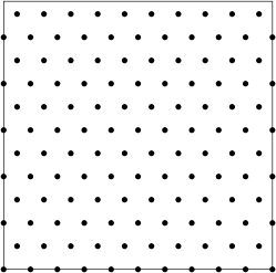
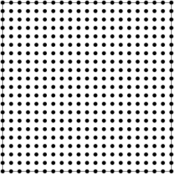
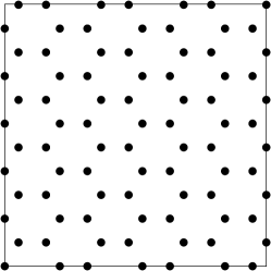
One set of disordered point processes that can exhibit hyperuniformity is the so-called class of determinantal point processes. A determinantal point process is a stochastic point process with a joint probability distribution given by the determinant of a finite-rank, positive, bounded, and self-adjoint operator. The determinantal form of the probability distribution is known to induce an effective repulsion amongst points in a realization of the corresponding point process, and these systems are therefore ideal candidates for hyperuniform point patterns. Examples of hyperuniform determinantal point processes have been documented both on the real line [45, 31, 8, 9] and in higher Euclidean dimensions [8, 9].
A particular example of a determinantal point process that exhibits hyperuniform behavior is generated by the so-called two-dimensional one-component plasma (see Figure 7);
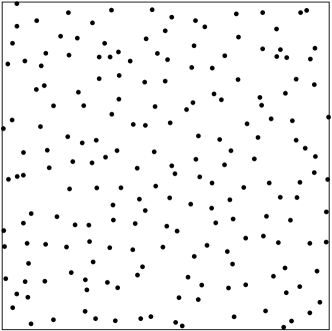
the total correlation function for this system is given by [10]:
| (92) |
and for the case , this system is equivalent to the Ginibre ensemble from random matrix theory [46, 47, 9]. The corresponding structure factor has the following small- behavior [10]:
| (93) |
and the long-range behavior of the total correlation function is governed by a Gaussian. This point process extends naturally to higher dimensions but does not retain any connection to random matrix theory.
Gabrielli and coworkers [48] have shown that the so-called “pinwheel” tiling [49] of the plane generates a hyperuniform point pattern. The pinwheel tiling is constructed by iteratively performing “decomposition” and “inflation” processes on right triangles with sides of lengths 1, 2, and . A point pattern is then obtained by randomly placing a point in each elementary triangle, and because the tiles appear in infinitely many orientations, the resulting point process is statistically homogeneous and isotropic333There is to date no rigorous proof of homogeneity for the point process generated by the pinwheel tiling; however, the current empirical evidence suggests that this claim is likely true [48]. The rotational invariance of the point pattern is experimentally manifested by a diffraction pattern consisting of uniform rings rather than isolated Bragg peaks.. Also considered by Gabrielli and coworkers is the Harrison-Zeldovich [50, 51] power spectrum for primordial density fluctuations in the Universe; the structure factor here scales linearly for small . Point patterns in three dimensions have been constructed that are consistent with this power spectrum [48]. Gabrielli, Joyce, and Torquato have also provided general constructions of hyperuniform point patterns from tilings of -dimensional Euclidean space by appropriately placing points per tile [52].
Two quasicrystalline structures in the plane that have been studied are the so-called Penrose and octagonal tilings. The Penrose tiling is composed of obtuse and acute rhombi, resulting in an overall five-fold rotational symmetry. Similarly, the octagonal tiling is obtained by laying down squares and rhombi in the plane and possesses an overall eight-fold rotational symmetry. These structures have recently received interest in the study and construction of photonic materials [53] that forbid propagation of electromagnetic radiation in some frequency range.
Torquato, Stillinger, and coworkers have introduced so-called -invariant processes, which are ideal methods for constructing hyperuniform point processes from known realizable pair correlation functions [54, 55, 56]. A -invariant process is defined for a chosen nonnegative via analytic extension with invariant form over a nonvanishing density range while keeping all other relevant macroscopic variables fixed. The upper limiting “terminal” density is the point above which the nonnegativity condition on the structure factor is violated, implying that at the terminal density the system is hyperuniform if realizable. Torquato and Stillinger [10] have calculated the asymptotic coefficients for a number of -invariant processes, and for completeness we include their results below in Tables 1, 2, and 3.
We finally remark that is has been conjectured that all saturated strictly jammed packings of hard spheres generate hyperuniform point patterns [10, 29]. A strictly jammed sphere packing is rigorously incompressible and nonshearable, and a saturated packing is one for which there is no space available to add another sphere. Of particular interest in this regard is the so-called maximally random jammed (MRJ) state, defined as the most disordered system (according to some well-defined order metric) among all strictly jammed packings [44]. Donev and coworkers [29] have provided strong numerical evidence to suggest that this disordered system is hyperuniform at saturation with a structure factor that is linear in as , suggesting that the conjecture is likely true.
5.3 New hyperuniform point patterns
We mention here the so-called “tunneled” crystals introduced by Torquato and Stillinger [40]; these periodic structures are formed by stacking two-dimensional honeycomb layers according to some repeated pattern in a manner similar to the construction of the FCC and HCP structures from triangular layers. The resulting crystals are unsaturated and yet hyperuniform due to the periodicity enforced by the stacking order [40]. The tunneled FCC crystal contains a periodic array of parallel linear tunnels that can be oriented in any one of six equivalent directions; in contrast, the tunneled HCP crystal contains tunnels with an overall zig-zag shape with three possible lateral directional orientations. As with the saturated parent packings, the tunneled FCC and tunneled HCP crystals have the same packing fractions; for more details on these systems, see [40].
Another novel application of this work in one dimension has involved the characterization of the so-called Fibonacci chain, which is a prototypical quasicrystal. A quasicrystal is a nonperiodic system whose correlation structure (i.e., and ) exhibits Bragg-like behavior, implying the presence of long-range order despite the absence of translational symmetry (see [57] and [58]). The Fibonacci chain is specifically composed of two length segments (“long” and “short” ) distributed iteratively on the line according to the following substitution rules: and . Upon taking the thermodynamic limit one obtains a quasiperiodic tiling of space; a point process can be generated by taking the endpoints of each segment (see Figure 3).
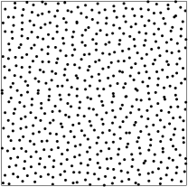
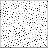
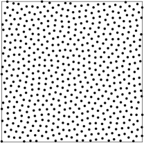
With regard to disordered hyperuniform point patterns, Batten, Stillinger, and Torquato [59] have numerically constructed examples of hyperuniform classical disordered ground states; these systems, which they describe as “stealth” materials, are prototypical heterogeneous media that completely suppress scattering of incident radiation for a specified set of wavevectors. The construction of these systems relies upon the minimization of a pairwise interaction , which can be represented in Fourier space as [59]:
| (94) |
where denotes the Lebesgue measure of the system domain, is the Fourier transform of a translationally invariant two-particle potential energy , and is defined by:
| (95) |
The function is chosen to be positive and bounded with compact support on some interval ; the authors in [59] also choose this function as isotropic, but the specific form of is largely inconsequential so long as it satisfies the properties enumerated above. By construction, the minimum of is then determined by minimizing in the interval , which by (95) requires that for all such wavenumbers. Therefore, it is clear that this construction algorithm inherently generates a hyperuniform point pattern. We remark that the degree of order in the resulting system is dependent on the ratio of the number of constrained degrees of freedom to the total number of degrees of freedom444The authors in [59] refer to the ratio that we denote here as by the letter . Since we have reserved the latter notation for the autocovariance function associated with the two-point probability , we adopt a different convention in this paper.. Figure 8 provides sample realizations of these hyperuniform disordered ground states for several values of ; note that the degree of global order in the system increases with increasing .
6 Higher-dimensional number variance coefficients and local volume fraction estimates
Here we provide extensive tables of asymptotic number variance coefficients for several Bravais lattice families up to , and these results, where appropriate, are compared to certain nonlattice ground states introduced by Cohn, Kumar, and Schürmann [65]. Estimates for the asymptotic volume fraction variance coefficients of the lattice systems may therefore be developed, providing insight into the dimensional asymptotic behavior of .
High-dimensional systems play an integral role in statistical physics. Of particular interest in this regard is the so-called sphere-packing problem, which has applications to abstract algebra, number theory, and communications theory [41]. For example, it is known that the optimal method of sending digital signals over noisy channels corresponds to the densest sphere packing in a high-dimensional space. Torquato and Stillinger have also provided evidence for a decorrelation principle of disordered packings in high-dimensional Euclidean spaces [24]. This principle states that as the dimension increases, all unconstrained correlations vanish, and any higher-order correlation functions may be written in terms of the number density and the pair correlation function function within some small error. The decorrelation principle appears to be robust, apparently incorporating a large number of point processes beyond sphere packings [61, 8, 9]. As a result, it is likely that glassy states of matter are intrinsically more stable than crystals in high dimensions and pack with a greater density [24], which should be contrasted with physical systems in two- and three-dimensions.
It is instructive to compare the estimate (76) for the asymptotic coefficient to an exact result for an analytically soluble system. We therefore consider the so-called “step-function” point process, defined at the two-point level (and therefore not uniquely) by:
| (96) |
where is the Heaviside step function and is an effective diameter for the point process. Note that the form of the pair correlation function (96) is exactly realized for an equilibrium system of hard spheres with diameter in the limit of low density. However, there is also strong theoretical and numerical evidence [56, 55, 62] to suggest that this pair correlation is realizable for nonzero densities up to the critical value . It is at this critical density that the structure factor approaches zero for small , and the system becomes hyperuniform555Above the critical density the structure factor for the step-function process falls below zero, signifying a violation of the Wiener-Khinchtine condition. The pair correlation function then ceases to be realizable as a point process [10].. The corresponding total correlation function is given by:
| (97) |
which admits the Fourier representation:
| (98) |
The asymptotic coefficient for the number variance at the critical density can be calculated analytically for this process; taking the -th moment of the total correlation function (97) and using the definition (24), we find:
| (99) |
The dimensional asymptotic behavior of this coefficient follows directly from the corresponding behavior of the gamma function; namely:
| (100) |
It is interesting to note that the pair correlation function (96) is also realizable as the infinite-dimensional limit of the so-called “ghost” random sequential addition (RSA) process at the saturation density [63]. This model is a generalization of the well-studied RSA process in which points are placed sequentially in some space according to a uniform distribution subject to the constraint that the points do not fall within some prescribed distance of either other points in the system or “ghost” points representing prior failed particle insertions. We remark that the resulting process represents a nonequilibrium hard-sphere packing. The result in (100) suggests a high-dimensional divergence in the local number variance for this system, and we more thoroughly explore the implications of this behavior at the end of this section.
An explicit calculation of the asymptotic coefficient can also be done for the step-function point process in low dimensions. The most difficult aspect of this calculation is the determination of the convolution in (59); an Fourier representation of this function is obtained by taking the Fourier transform of the convolution using (98) and the result:
| (101) |
We therefore find:
| (102) | |||||
We remark that there is no reason a priori to identify the particle radius with ; the length scale is imposed inherently by the structure of the underlying point process and is not affected by a “decoration” of the points via circumscription with spheres. However, it is computationally convenient to make this connection, and we additionally set .
For , the expression (102) simplies according to:
| (103) |
where at the critical density. Using (54) we find the following result for the asymptotic coefficient:
| (104) |
One can also verify directly from (103) that as expected for a hyperuniform medium. According to (100), the corresponding coefficient for the local number density is,
| (105) |
and applying the estimate (76) leads to the following upper bound on :
| (106) |
which we see is strictly fulfilled for this system.

It is therefore clear that the upper limit in (76) will generally not be obtained for a given random medium; however, this estimate does provide some insight into the dimensional asymptotic properties of . Figure 9 shows the behavior of the estimate (76) for the step-function process as the dimension of the system increases. We observe that, unlike the divergent behavior in the coefficient , decreases at most monotonically as the dimension increases and vanishes asymptotically for large dimensions666It should be noted that monotonicity of the upper bound (76) for is not generally true for all hyperuniform systems. However, this issue does not affect our conclusions concerning the dimensional asymptotic behavior of this estimate.. It is known that fluctuations in the local number density in a spherical observation window cannot grow more slowly than the surface area of the window [30, 10], and if this claim is also true for local volume fraction fluctuations, then it follows that in high dimensions the local volume fraction for large windows is almost surely equal to the global volume fraction in the system.
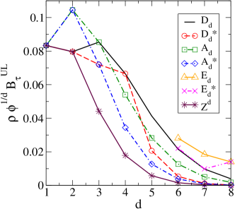
Right: Corresponding scaling for the estimate of the asymptotic local volume fraction variance coefficient .
One expects that this behavior is quite general for other disordered systems by invoking a so-called decorrelation principle. As discussed by Torquato and Stillinger [24], the decorrelation principle states that in the high-dimensional limit, unconstrained correlations asymptotically vanish, and knowledge about higher-order correlations ( for ) can be inferred directly from knowledge of the pair correlation function and the number density . In other words, long-range fluctuations in , and therefore , should diminish as the dimension of the system increases; since these fluctuations are responsible for enforcing the constraint:
| (107) |
it follows that the value of this integral becomes sequentially less negative in higher dimensions. Therefore, we expect that for general heterogeneous media, including but not limited to the step-function process above, as in constrast to the behavior of . It is in this sense that we claim that high-dimensional hyperuniform heterogeneous media can be generated from increasingly disordered point processes and yet possess inherently ordered microstructural information in terms of the local volume fraction.
| 1 | 0.08333 (1) | 0.08333 (1) | 0.08333 (1) |
|---|---|---|---|
| 2 | 0.12910 () | 0.12709 () | 0.12709 () |
| 3 | 0.16115 () | 0.15569 () | 0.15560 () |
| 4 | 0.18767 () | 0.17733 () | 0.17689 () |
| 5 | 0.21273 () | 0.19579 () | 0.19453 () |
| 6 | 0.23925 () | 0.21327 () | 0.21036 () |
| 7 | 0.27012 () | 0.23170 () | 0.22569 () |
| 8 | 0.30904 () | 0.25258 () | 0.24144 () |
| 1 | 0.08333 (1) | 0.08333 (1) | - |
| 2 | 0.12910 () | 0.12910 () | - |
| 3 | 0.15569 () | 0.15560 () | - |
| 4 | 0.17488 () | 0.17488 () | - |
| 5 | 0.19103 () | 0.19070 () | - |
| 6 | 0.20653 () | 0.20485 () | 0.20221 () |
| 7 | 0.22327 () | 0.21845 () | 0.21172 () |
| 8 | 0.24329 () | 0.23236 () | 0.21746 () |
| 1 | - | ||
| 2 | - | ||
| 3 | - | ||
| 4 | - | ||
| 5 | - | ||
| 6 | 0.20195 () | ||
| 7 | 0.21119 () | ||
| 8 | 0.21746 () |
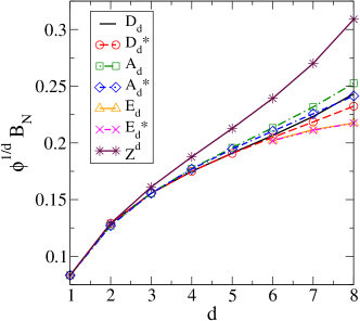
The analysis of periodic structures is seemingly more complicated. These systems inherently contain long-range order, and there is no reason a priori for a decorrelation principle to apply. Nevertheless, the same qualitative trends are observed for these systems as seen in Figure 10, which compares the asymptotic coefficients and for several lattice families across dimensions; the results for the number variance coefficients are also collected in Table 4. Note that for a meaningful comparison among lattice families we have scaled the coefficients appropriately to remove the dependence on the parameter , which amounts to mapping and according to (22) and (52); the factor of is included in the rescaling of for computational convenience. As with the step-function process, the coefficients for the local number density increase monotonically and likely diverge asymptotically with respect to increasing dimension. Fluctuations in the local volume fraction generally decrease for sufficiently large dimensions, although not necessarily monotonically. It is interesting to note that the asymptotic number variance coefficient for a Bravais lattice is apparently larger than its dual, and this trend also appears to hold for the local volume fraction. However, it seems that the integer lattices may surprisingly possess the smallest volume fraction fluctuations among these lattices despite having significantly smaller packing fractions. This behavior arises mathematically from the rapidly diminishing volume fraction for the integer lattice in high dimensions, which has the effect of drastically lowering the upper bound to the scaled local volume fraction asymptotic coefficient relative to other lattices. We remark, however, that the curves in Figure 10 are simply estimates of the volume fraction fluctuations, meaning that global minimization of cannot be readily ascertained from these results. However, we can conclude that it is not necessarily true that minimizing fluctuations in the local number density incidentally minimizes fluctuations in the local volume fraction for a heterogeneous medium.
Cohn and Kumar [60] have also discussed nonlattice packings that possess lower ground-state energies than the densest Bravais lattices for certain classes of soft-core pair potentials. Specifically, they consider in five and seven dimensions certain stacking variants, first introduced by Conway and Sloane [64], of the densest Bravais lattices that possess lower ground state energies for the so-called Gaussian core model, which involves a pair potential . We adopt their notation for these energy-minimizing nonlattices and . Since the Gaussian core potential and the overlap potential governing the number variance are both completely monotonic (the former in the squared distance ), we expect the ground-state structures of these interactions to be similar [33]. With this notion in mind we mention that the nonlattice packings and actually belong to one-parameter families and [65] of packings, the theta series for which are given by:
| (108) | |||||
| (109) | |||||
The nonlattices and are obtained by setting and , respectively. Following Cohn, Kumar, and Schürmann [65], we define two structures to be formally dual if their pair correlation functions have the same relationship as Poisson summation gives for a Bravais lattice and its reciprocal lattice. For the families and , formal duality is obtained by replacing with ; this statement implies that formally self-dual packings occur for .
| Packing | |
|---|---|
| 0.19099 | |
| 0.19069 | |
| 0.21037 | |
| 0.21115 | |
| 0.21090 | |
| 0.21037 |
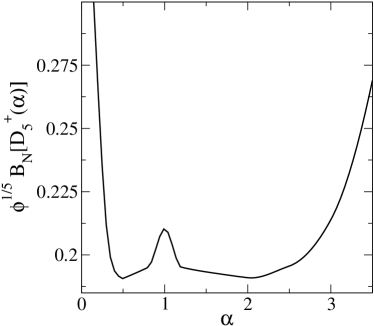
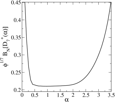
For , we have numerically found that the asymptotic number variance coefficient for is a local minimum within the family; the formal dual may be the global minimum (see Figure 11). In fact, it appears that may possess a lower number variance coefficient than , albeit by an unusually narrow margin (see Tables 4 and 5). Using approximately the first terms of the theta series for both structures, we have found that and , where the listed errors represent standard errors from a linear regression analysis. Since the theta series for is distinct from that of and since a lattice determines a theta series (but not conversely), we expect that this difference, though small, is significant and not an artifact of numerical imprecision. This conclusion is corroborated by the observation that the numerical values for the asymptotic number variance coefficients above are empirically constant when incorporating additional terms from the theta series. We remark that the formally self-dual packing appears to be a local maximum in the family with respect to the number variance coefficient. In contrast, neither nor its formal dual appear to be extrema among the packings in the family; the global minimum is apparently the formally self-dual nonlattice as shown in Figure 11. However, , , , and any nonlattices in between possess lower number variance coefficients than (Tables 4 and 5), suggesting that the dual of the densest Bravais lattice in a given dimension may no longer be even a local minimum with respect to the number variance in higher dimensions. Note also that if and are indeed the global minima for the number variance in five and seven dimensions, respectively, then it follows that the duals of these systems should minimize the Epstein zeta function of argument . This observation is a direct result of the equivalence between the number variance and Epstein zeta function established by Torquato and Stillinger [10].
7 Concluding remarks
We have extended the notion of hyperuniformity to incorporate both stochastic point processes and two-phase random heterogeneous media. In the case of microstructures of impenetrable spheres, an upper bound can be established on the asymptotic fluctuations in the local volume fraction in terms of the corresponding results for the local number variance of the underlying point process. The information contained in this estimate is particularly applicable for high-dimensional systems, where decorrelation reduces long-range spatial fluctuations in the system and decreases the leading-order term in the asymptotic local volume fraction variance. Furthermore, we have provided an extensive characterization of hyperuniform point processes in several dimensions; our results indicate that the asymptotic coefficient may provide a quantitative order metric describing the extent of spatial uniformity. This order metric faithfully reproduces our physically intuitive ordering of low-dimensional structures and has surprising implications for understanding order in high-dimensional systems. By studying several lattice families up to , we have shown that a Bravais lattice generally possesses a higher asymptotic number variance coefficient than its dual. Furthermore, in dimensions five and seven we have shown for the first time that it is possible for a nonlattice to possess a lower asymptotic number variance coefficient than any Bravais lattice, and the corresponding duals of these nonlattices should therefore also minimize the Epstein zeta function for argument values .
One promising direction for future research is to construct hyperuniform point patterns with targeted values of the asymptotic number variance coefficient [10]. This problem can be expressed in terms of an optimization scheme, whereby one either seeks:
| (110) |
where is given by (89), or attempts to minimize the square fluctuation of this objective function from a target value. The spatial averaging in (110) is necessary to smooth the small-scale fluctuations that arise from the volume-average interpretation of the number variance fluctuations, which is applicable for a single point pattern and therefore appropriate for the optimization scheme. Since we have established a quantitative order metric in this paper based on the asymptotic coefficient for the number variance, it is feasible that one could develop new types of quasiperiodic or disordered structures with similar applications to the materials studied by Batten, Stillinger, and Torquato [59].
Additionally, it is an open problem to systematically construct a heterogeneous medium that is hyperuniform with respect to the local volume fraction. One feasible approach in this regard is to utilize so-called “inverse construction” algorithms [66, 67, 68, 69]. However, this issue is complicated by the fact that not every heterogeneous medium can be derived from an underlying stochastic point process; in other words, it is not possible to construct an arbitrary microstructure by decorating some point process in the space. One therefore seeks autocovariance functions that are realizable as heterogeneous media, meaning that there exists a binary stochastic process with autocovariance function . Several necessary but not sufficient conditions for realizability have been given in the literature [70, 71], and it known that numerical constructions of heterogeneous systems are sensitive to the realizability of the -point probabilities [68, 69]. Further research in this area is certainly warranted.
References
References
- [1] Hansen J-P and McDonald I R, 1986 Theory of Simple Liquids (New York: Academic Press)
- [2] Pietronero L, Gabrielli A and Labini F S, Statistical physics for cosmic structures, 2002 Physica A 306 395
- [3] Warr S and Hansen J-P, Relaxation of local density fluctuations in a fluidized granular medium, 1996 Europhys. Lett. 36 589
- [4] Wax A, Yang C, Backman V, Badizadegan K, Boone C W, Dasari R R and Feld M S, Cellular organization and substructure measured using angle-resolved low-coherence interferometry, 2002 Biophys. J. 82 2256
- [5] Kendall D G, On the number of lattice points inside a random oval, 1948 Quarterly J. Math. 19 1
- [6] Kendall D G and Rankin R A, On the number of points of a given lattice in a random hypersphere, 1953 Quarterly J. Math. 4 178
- [7] Bleher P M, Dyson F J and Lebowitz J L, Non-Gaussian energy level statistics for some integrable systems, 1993 Phys. Rev. Lett. 71 3047
- [8] Torquato S, Scardicchio A and Zachary C E, Point processes in arbitrary dimension from fermionic gases, random matrix theory, and number theory, 2008 J. Stat. Mech.: Theory and Expt. P11019
- [9] Scardicchio A, Zachary C E and Torquato S, Statistical properties of determinantal point processes in high-dimensional Euclidean spaces, 2009 Phys. Rev. E 79 041108
- [10] Torquato S and Stillinger F H, Local density fluctuations, hyperuniformity, and order metrics, 2003 Phys. Rev. E 68 041113
- [11] Stoyan D, Kendall W S and Mecke J, 1995 Stochastic Geometry and its Applications (New York: Wiley)
- [12] Torquato S and Stell G, Microstructure of two-phase random media. I. The n-point probability functions, 1982 J. Chem. Phys. 77 2071
- [13] Torquato S and Stell G, Microstructure of two-phase random media. II. The Mayer-Montroll and Kirkwood-Salsburg hierarchies, 1983 J. Chem. Phys. 78 3262
- [14] Torquato S, 2002 Random Heterogeneous Materials: Microstructure and Macroscopic Properties (New York: Springer)
- [15] Debye P, Anderson H R and Brumberger H, Scattering by an inhomogeneous solid. II. The correlation function and its application, 1957 J. Appl. Phys. 28 679
- [16] Torquato S and Lado F, Trapping constant, thermal conductivity, and the microstructure of suspensions of oriented spheriods, 1991 J. Chem. Phys. 94 4453
- [17] Bayer B E, Relation between granularity and density for a random-dot model, 1964 J. Opt. Soc. Am. 54 1485
- [18] Lu B and Torquato S, Photographic granularity: mathematical formulation and effect of impenetrability of grains, 1990 J. Opt. Soc. Am. A 7 717
- [19] Fishman R S, Kurtze D A and Bierwagen G P, The effects of density fluctuations in organic coatings, 1992 J. Appl. Phys. 72 3116
- [20] Torquato S, Modeling of physical properties of composite materials, 2000 Int. J. Solids Structures 37 411
- [21] Lu B and Torquato S, Local volume fraction fluctuations in heterogeneous media, 1990 J. Chem. Phys. 93 3452
- [22] Quintanilla J and Torquato S, Local volume fraction fluctuations in random media, 1997 J. Chem. Phys. 106 2741
- [23] Quintanilla J and Torquato S, Local volume fraction fluctuations in periodic heterogeneous media, 1999 J. Chem. Phys. 110 3215
- [24] Torquato S and Stillinger F H, New conjectural lower bounds on the optimal density of sphere packings, 2006 Expt. Math. 15 307
- [25] Lebowitz J L, Charge fluctuations in Coulomb systems, 1983 Phys. Rev. A 27 1491
- [26] Landau L D and Lifshitz E M, 1980 Statistical Physics (New York: Pergamon Press)
- [27] Martin Ph A and Yalcin T, The charge fluctuations in classical Coulomb systems, 1980 J. Stat. Phys. 22 435
- [28] Torquato S, 2009 in preparation
- [29] Donev A, Stillinger F H and Torquato S, Unexpected density fluctuations in jammed disordered sphere packings, 2005 Phys. Rev. Lett. 95 090604
- [30] Beck J, Irregularities of distribution. I, 1987 Acta Math. 159 1
- [31] de Coninck J, Dunlop F and Huillet T, On the correlation structure of some random point processes on the line, 2008 Physica A 387 725
- [32] Sarnak P and Strömbergsson A, Minima of Epstein’s zeta function and heights of flat tori, 2006 Invent. math. 165 115
- [33] Torquato S and Stillinger F H, New duality relations for classical ground states, 2008 Phys. Rev. Lett. 100 020602
- [34] Rankin R A, A minimum problem for the Epstein zeta function, 1953 Proc. Glasg. Math. Assoc. 1 149
- [35] Cassels J W S, On a problem of Rankin about the Epstein zeta function, 1959Proc. Glasg. Math. Assoc. 4 73; 1963 6 116
- [36] Diananda P H, Notes on two lemmas concerning the Epstein zeta-function, 1964 Proc. Glasg. Math. Assoc. 6 202
- [37] Ennola V, A lemma about the Epstein zeta-function, 1964 Proc. Glasg. Math. Assoc. 6 198
- [38] Ennola V, On a problem about the Epstein zeta function, 1964 Proc. Camb. Philos. Soc. 60 855
- [39] Torquato S and Sen A K, Conductivity tensor of anisotropic composite media from the microstructure, 1990 J. Appl. Phys. 67 1145
- [40] Torquato S and Stillinger F H, Toward the jamming threshold of sphere packings: Tunneled crystals, 2007 J. Appl. Phys. 102 093511
- [41] Conway J H and Sloane N J A, 1999 Sphere Packings, Lattices and Groups 3rd edn (New York: Springer)
- [42] Sloane N J A, Theta series and magic numbers for diamond and certain ionic crystal structures, 1987 J. Math. Phys. 28 1653
- [43] Steinhardt P J, Nelson D R and Ronchetti M, Bond-orientational order in liquids and glasses, 1983 Phys. Rev. B 28 784
- [44] Torquato S, Truskett T M and Debenedetti P G, Is random close packing of spheres well-defined?, 2000 Phys. Rev. Lett. 84 2064
- [45] Costin O and Lebowitz J L, On the construction of particle distributions with specified single and pair densities, 2004 J. Phys. Chem. B 108 19614
- [46] Ginibre J, Statistical ensembles of complex, quaternion, and real matrices, 1965 J. Math. Phys. 6 440
- [47] Mehta M L, 2004 Random Matrices 3rd edn (Amsterdam: Elsevier Academic Press)
- [48] Gabrielli A, Jancovici B, Joyce M, Lebowitz J L, Pietronero L and Labini F S, Generation of primordial cosmological perturbations from statistical mechanical models, 2003 Phys. Rev. D 67 043506
- [49] Radin C, The pinwheel tilings of the plane, 1994 Ann. Math. 139 661
- [50] Harrison E R, Fluctuations at the threshold of classical cosmology, 1970 Phys. Rev. D 1 2726
- [51] Zeldovich Y B, A hypothesis, unifying the structure and the entropy of the Universe, 1972 Mon. Not. R. Astron. Soc. 160 1
- [52] Gabrielli A, Joyce M and Torquato S, Tilings of space and superhomogeneous point processes, 2008 Phys. Rev. E 77 031125
- [53] Florescu M, Torquato S and Steinhardt P J, Complete band gaps in 2D photonic quasicrystals, 2009 Phys. Rev. B in press
- [54] Torquato S and Stillinger F H, Controlling the short-range order and packing densities of many-particle systems, 2002 J. Phys. Chem. B 106 8354; 106 11406
- [55] Stillinger F H, Torquato S, Eroles J M and Truskett T M, Iso- processes in equilibrium statistical mechanics, 2001 J. Phys. Chem. B 105 6592
- [56] Sakai H, Torquato S and Stillinger F H, Equi- sequences of systems derived from the square-well potential, 2002 J. Chem. Phys. 117 297
- [57] Levine D and Steinhardt P J, Quasicrystals: A new class of ordered structures, 1984 Phys. Rev. Lett. 53 2477
- [58] Janot C, 1994 Quasicrystals: A Primer 2nd edn (Oxford: OUP)
- [59] Batten R D, Stillinger F H and Torquato S, Classical disordered ground states: Super-ideal gases and stealth and equi-luminous materials, 2008 J. Appl. Phys. 104 033504
- [60] Cohn H and Kumar A, Counterintuitive ground states in soft-core models, 2008 Phys. Rev. E 78 061113
- [61] Zachary C E, Stillinger F H and Torquato S, Gaussian core model phase diagram and pair correlations in high Euclidean dimensions, 2008 J. Chem. Phys. 128 224505
- [62] Crawford J, Torquato S and Stillinger F H, Aspects of correlation function realizability, 2003 J. Chem. Phys. 119 7065
- [63] Torquato S and Stillinger F H, Exactly solvable disordered sphere-packing model in arbitrary-dimensional Euclidean spaces, 2006 Phys. Rev. E 73 031106
- [64] Conway J H and Sloane N J A, What are all the best sphere packings in low dimensions?, 1995 Discrete Comput. Geom. 13 383
- [65] Cohn H, Kumar A and Schürmann A, Ground states and formal duality relations in the Gaussian core model, 2009 submitted for publication
- [66] Yeong C L Y and Torquato S, Reconstructing random media, 1998 Phys. Rev. E 57 495
- [67] Yeong C L Y and Torquato S, Reconstructing random media: II. Three-dimensional from two-dimensional cuts, 1998 Phys. Rev. E 58 224
- [68] Jiao Y, Stillinger F H and Torquato S, Modeling heterogeneous materials via two-point correlation functions: Basic principles, 2007 Phys. Rev. E 76 031110
- [69] Jiao Y, Stillinger F H and Torquato S, Modeling heterogeneous materials via two-poin correlation functions: II. Algorithmic details and applications, 2008 Phys. Rev. E 77 031135
- [70] Torquato S, Exact conditions on physically realizable correlation functions of random media, 1999 J. Chem. Phys. 111 8832
- [71] Torquato S, Necessary conditions on realizable two-point correlation functions of random media, 2006 Ind. Eng. Chem. Res. 45 6923