Self-optimized Coverage Coordination in Femtocell Networks

Abstract

This paper proposes a self-optimized coverage coordination scheme for two-tier femtocell networks, in which a femtocell base station adjusts the transmit power based on the statistics of the signal and the interference power that is measured at a femtocell downlink. Furthermore, an analytic expression is derived for the coverage leakage probability that a femtocell coverage area leaks into an outdoor macrocell. The coverage analysis is verified by simulation, which shows that the proposed scheme provides sufficient indoor femtocell coverage and that the femtocell coverage does not leak into an outdoor macrocell.

I Introduction

Femtocell technology has been emerging as a solution to the increase of both capacity and coverage while reducing both the capital expenditures and operating expenses of cellular networks. As femtocells share spectrum with macrocell networks, controlling the cross-tier interference between femto- and macrocells is need to be considered first in the enhancement of coverage and capacity. In addition, since a network operator may not be able to control femtocell locations, it is necessary for femtocells to sense the radio environment around them and carry out the self-configuration and self-optimization [1]-[3] of radio parameters from the moment they are set up by a consumer.

Conventional dynamic cell sizing schemes, which adjust the transmit power of a base station (BS) [4][5] or both the transmit power and antenna beam forming [6], have been developed to improve the overall system capacity compared to that of a fixed cell sizing scheme. These approaches are not suitable for a macro/femto overlaid cell structure, where femtocell coverage must be controlled so it does not interfere with the outdoor macrocell. In order to achieve this goal, Claussen et al. [7] proposed a femtocell coverage coordination method that adjusts the femtocell pilot power, based on the number of handover events from outdoor passing, and the indoor users, which is robust against the varying size and shape of buildings. However, outdoor users may already experience inferior link quality during the time that a femtocell BS reduces its transmit power after recognizing the handover events of outdoor users. In particular, in a private access scenario that serves only registered users, the unauthorized users near a femtocell have a serious increase in the call drop rate or reduction of data rate. Moreover, the procedure that reconnects the rejected outdoor user to the macrocell may induce an additional handover, which causes a considerable amount of data transmission delay as well as packet loss in a packet switched cellular network with hard handovers, such as IEEE 802.16e WiMAX and HSDPA [8][9]. Therefore, this problem is severe for delay- and packet-loss-sensitive real-time applications such as Voice over Internet Protocol (VoIP).

This paper proposes a coverage coordination scheme that is based on the statistics of the signal and interference power measured at a femtocell downlink (as opposed to the scheme based on handover events) to prevent any handover of outdoor users in advance. The proposed scheme comprises both the self-configuration and self-optimization of femtocell pilot transmit power. With a self-configuration function, a femtocell BS initiates its transmit power based on the measurement of interference from neighboring BSs in a manner that achieves a roughly constant cell coverage. The femtocell BS then performs a self-optimization function that continually adjusts the transmit power so that the femtocell coverage does not leak into an outdoor area while sufficiently covering an indoor femtocell area.

II Downlink Transmit Power Control

This study considers a two-tier cellular network composed of overlaid macrocells and underlaid femtocells in which both cells use the same frequency channel. A femtocell BS is located at the center of a building with radius $r_{b}$. Both BS and user are equipped with an omni-directional antenna. The femtocell BS creates cell coverage with radius $r_{f}$, which is adaptively adjusted by the proposed transmit power control in order to correspond to the building area i.e., $r_{f}=r_{b}$. The transmit power control is composed from a two step procedure, where the femtocell BS initially self-configures its power and self-optimizes cell coverage by using transmit power control based on the measurements of radio environments.

II-A Initial Self-configuration

A femtocell BS measures the average received power of pilot (over multiple frames to average out fast fading effect) from the neighboring macrocell and femtocell BSs on a neighboring BS list. The femtocell then chooses the strongest pilot power, $I_{b,max}$, among them. The femtocell BS configures its transmit pilot power such that the received pilot power from the femtocell BS and the strongest macrocell BS are identical on average at an initial cell radius of $r_{ini}$, i.e., $r_{f}=r_{ini}$. The Appendix shows that $I_{b,max}$ is nearly identical to the interference power from the strongest macrocell both measured by and averaged over the users located at the initial cell edge. Thus, the initial femtocell pilot power $P_{f,ini}$ (dBm) is determined such that the femtocell BS power received at $r_{ini}$ is equal to $I_{b,max}$, as follows:

$$P_{f,ini}=\min\left(I_{b,max}+L\left(r_{ini}\right),P_{\max}\right).$$ (1)

Here, $P_{\max}$ and $L$ are maximum femtocell pilot power and path loss, respectively. The initial self-configuration only provides the initial cell coverage of a femtocell, which is refined by the following self-optimized power control.

II-B Self-optimized Power Control

A femtocell BS measures the level of other-cell interference $I_{u}(0)$ that is received from neighboring macrocells and femtocell BSs. The femtocell BS evaluates the received interference-plus-noise power $Z_{u}(0)=10\log_{10}(I_{u}(0)+W)$, where $W$ is the thermal noise power. The femtocell BS collects the time-averaged received power $Q^{(i)}$ in dBm, which is measured by each femtocell user during the $i$th iteration and is fed back to the currently linked femtocell BS. Based on the decision variable $\Gamma^{(i)}=\overline{Q}^{(i)}-Z_{u}(0)$, where $\overline{Q}^{(i)}$ is the averaged $Q^{(i)}$ over femtocell users, the transmit pilot power of the femtocell BS at the $i$th iteration is updated by

$$P_{f}^{(i+1)}=\left\{\begin{array}[]{ll}\min\left(P_{f}^{(i)}+\Delta P,P_{\max}\right)&\textrm{for~{}~{}}\Gamma^{(i)}\leq\Gamma_{th},\\ \min\left(P_{f}^{(i)}-\Delta P,P_{\max}\right)&\textrm{otherwise}.\end{array}\right.$$ (2)

Here, $\Delta P$ is the power control step in dB. $P_{f}^{(i+1)}$ is determined by comparing $\Gamma^{(i)}$ with a threshold $\Gamma_{th}=\Gamma_{0}+\Gamma_{\Delta}$, where $0\leq\Gamma_{\Delta}\leq\Gamma_{\Delta,\max}$. In order to make this power control scheme work properly, it is essential to set the threshold appropriately, that is, determining $\Gamma_{0}$ and $\Gamma_{\Delta,\max}$.

II-B1 Statistical Threshold $\Gamma_{0}$

$\Gamma_{0}$ is obtained from the statistical characteristics of $\Gamma^{(i)}$. Under the approximation that femtocell users are uniformly distributed over a circular femtocell with a radius of $r_{f}$ at the $i$th iteration, the probability density function (PDF) of random variable $D$, which represents the distance between the femtocell BS and user, is given as $f_{D}(d)=2d\big{/}({r_{f}^{(i)}}^{2}-\varepsilon_{0}^{2}),~{}d\in[\varepsilon_{0},{r_{f}^{(i)}}^{2}]$, where $\varepsilon_{0}$ is the minimum $D$. Here, all radii and distances are in meters. Both the outdoor and indoor path loss in dB are modeled as $L(D)=A_{s}+10n\log\left(D/d_{s}\right)$, where $n$ and $A_{s}$ denote the path loss exponent and the path loss at a reference distance of $d_{s}=1$ m, respectively. For the outdoor-to-indoor path loss, the wall penetration loss $L_{p}$ is added to $L(D)$. When $r_{f}^{(i)}\leq r_{b}$, the time-averaged received power of a femtocell user is given by $Q^{(i)}=P_{f}^{(i)}-L\left(D\right)$. Then, from the PDF of $D$, the PDF of $Q^{(i)}$ is given as

$$f_{Q^{(i)}}(q)=10^{\frac{P_{f}^{(i)}-A_{s}-q}{5n}}\ln 10\Big{/}(5n({r_{f}^{(i)}}^{2}-\varepsilon_{0}^{2})),~{}q\in\left[P_{f}^{(i)}-L(r_{f}^{(i)}),P_{f}^{(i)}-L(\varepsilon_{0})\right].$$ (3)

The expected value of $Q^{(i)}$ is given by

$$E\left[Q^{(i)}\right]=5n/\ln 10+P_{f}^{(i)}-A_{s}-10n({r_{f}^{(i)}}^{2}\log r_{f}^{(i)}-\varepsilon_{0}^{2}\log\varepsilon_{0})\Big{/}({r_{f}^{(i)}}^{2}-\varepsilon_{0}^{2}).$$ (4)

Let denote $\overline{I}_{u}(D)$ as the other-cell interference averaged over the users uniformly located on a circumference of radius of $D$ centered at their femtocell BS. Since $I_{u}(0)\approx\overline{I}_{u}(D)$ for $D<0.5d_{b,i}$ from the Appendix, $I_{u}(0)\approx\overline{I}_{u}(r_{f}^{(i)})$; therefore, $\Gamma^{(i)}$ is approximated as

$$\Gamma^{(i)}=\overline{Q}^{(i)}-Z_{u}(0)\approx E\left[Q^{(i)}\right]-\overline{Z}(r_{f}^{(i)}),$$ (5)

where $\overline{Z}(r_{f}^{(i)})=10\log_{10}\left(\bar{I}_{u}(r_{f}^{(i)})+W\right)$. Furthermore, when $r_{f}^{(i)}<r_{b}$, the average CINR of the user located at a femtocell edge is equal to a CINR threshold $\gamma_{th}$, i.e., $Q^{(i)}(r_{f}^{(i)})-\overline{Z}(r_{f}^{(i)})=\gamma_{th}$. From this constraint, $\Gamma^{(i)}$ can be further approximated as follows:

$$\Gamma^{(i)} \approx E\left[Q^{(i)}\right]-Q^{(i)}(r_{f}^{(i)})+\gamma_{th}$$ (6)

$$\mathop{=}\limits^{\left(a\right)} 5n/\ln 10+\gamma_{th}-\tfrac{10n\varepsilon_{0}^{2}}{{r_{f}^{(i)}}^{2}-\varepsilon_{0}^{2}}\log\tfrac{r_{f}^{(i)}}{\varepsilon_{0}},~{}\textrm{for}~{}~{}r_{f}^{(i)}<r_{b},$$ (7)

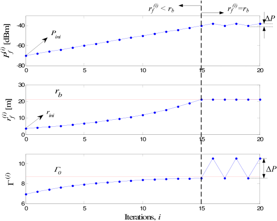
Figure 2: A change of transmit power, femtocell coverage, and $\Gamma^{(i)}$, using the proposed power control with $\Gamma_{th}=\Gamma_{0}$ and $\Delta P$=2 dB.

where (a) follows from (4) and the equation $Q^{(i)}=P_{f}^{(i)}-L\left(D\right)$. This interestingly shows that $\Gamma^{(i)}$ depends only on $r_{f}^{(i)}$, and increases and converges to $\Gamma_{0}=\frac{5n}{\ln 10}+\gamma_{th}$ as $r_{f}^{(i)}$ increases (see the $\Gamma^{(i)}$ graph $(i\leq 15)$ in Fig. 2).

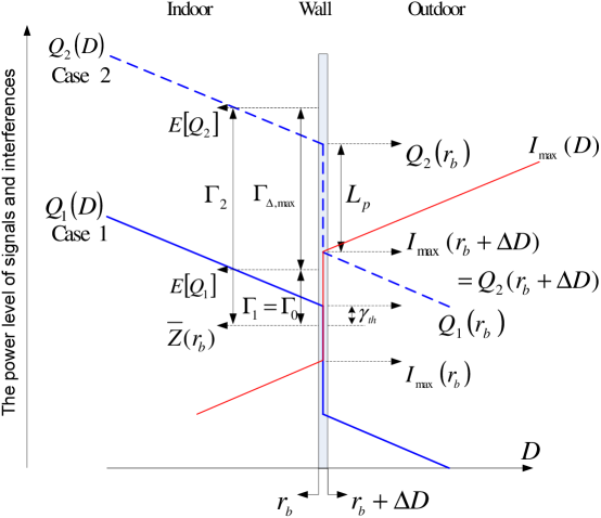
Figure 3: Wall penetration loss $L_{p}$ enables a femtocell BS to utilize the additional threshold $\Gamma_{\Delta}$, $0\leq\Gamma_{\Delta}\leq\Gamma_{\Delta,\max}$ (Case 1: $r_{f}=r_{b}$, Case 2: $r_{f}=r_{b}+\Delta D$).

Fig. 2 describes an example of the coverage adaptation process that uses the power control scheme with $\Gamma_{th}=\Gamma_{0}$. When $r_{f}^{(i)}<r_{b}~{}(i<15)$, $\Gamma^{(i)}$ is determined by (7) and it is less than $\Gamma_{0}$. Therefore, as the iteration index $i$ increases, the transmit power $P_{f}^{(i)}$ increases, and the femtocell coverage $r_{f}^{(i)}$ extends to a building wall. The first time that $r_{f}^{(i)}$ is equal to $r_{b}~{}(i=15)$, $\Gamma^{(15)}$ is a little less then $\Gamma_{0}$, which leads to an increase in $P_{f}^{(i)}$. However, contrary to the case of $i<15$, the increase of transmit power no longer extends the femtocell coverage to the outdoors, i.e., $r_{f}^{(i+1)}=r_{f}^{(i)}$, until the transmit power becomes large enough to overcome the additional path loss due to wall penetration so that femtocell coverage leaks into the outdoor region (see Case 2 in Fig. 3). This constant cell coverage causes constant average interference-plus-noise power at the cell edge, i.e., $\overline{Z}(r_{f}^{(i+1)})=\overline{Z}(r_{f}^{(i)})$, thus $\Gamma^{(i+1)}-\Gamma^{(i)}=E[Q^{(i+1)}]-E[Q^{(i)}]$ from (5). Additionally, $r_{f}^{(i+1)}=r_{f}^{(i)}$ results in $E[Q^{(i+1)}]-E[Q^{(i)}]=P_{f}^{(i+1)}-P_{f}^{(i)}$ from (4), and $P_{f}^{(i+1)}-P_{f}^{(i)}=\pm\Delta P$ from (2), i.e., $\Gamma^{(i+1)}-\Gamma^{(i)}=\pm\Delta P$. Therefore, $\Gamma^{(i)}$ is reformulated as

$$\Gamma^{(i+1)}=\left\{\begin{array}[]{ll}\Gamma^{(i)}+\Delta P&\textrm{for}~{}~{}\Gamma^{(i)}\leq\Gamma_{th},\\ \Gamma^{(i)}-\Delta P&\textrm{otherwise}\end{array}\right.~{}\textrm{for}~{}~{}r_{f}^{(i)}=r_{b}.$$ (8)

According to this equation, $\Gamma^{(16)}=\Gamma^{(15)}+\Delta P>\Gamma_{0}$ on the assumption that $\Delta P>\Gamma_{0}-\Gamma^{(15)}$ (more iterations will provide $\Gamma^{(i)}>\Gamma_{0}$ when $\Delta P<\Gamma_{0}-\Gamma^{(15)}$), and $P_{f}^{(i)}$ increases no more than $P_{f}^{(16)}$. Thus, $\Gamma_{th}$, which is set to $\Gamma_{0}$, provides femtocell coverage that corresponds to the building area, i.e., $r_{f}=r_{b}$. It is important to note that this method is effective irrespective of the building’s size, because $\Gamma_{0}=\frac{5n}{\ln 10}+\gamma_{th}$ and $\Gamma^{(i)}$ given by (7) or (8) are independent of $r_{b}$.

II-B2 Maximum Additional Threshold $\Gamma_{\Delta,\max}$

From Fig. 2, we can observe that when the threshold $\Gamma_{th}$ higher than $\Gamma_{0}$ does not increase transmit power $P_{f}^{(i)}$ up to the level at which femtocell coverage leaks into an outdoor area, a downlink CINR of femtocell is improved while $r_{f}^{(i)}=r_{b}$. From this observation we define $\Gamma_{\Delta,\max}$ as the maximum increase, which satisfies the condition $r_{f}^{(i)}=r_{b}$, from the basic threshold $\Gamma_{0}$.

$\Gamma_{\Delta,\max}$ is designed from the two cases of femtocell coverage described in Fig. 3. In Case 1, femtocell coverage is extended to a building wall, i.e., $r_{f}=r_{b}$, by using $\Gamma_{th}=\Gamma_{0}$. Increasing the transmit power of femtocell BS more than that of Case 1 results in Case 2, in which the femtocell coverage begin to leak into an outdoor region, i.e., $r_{f}=r_{b}+\Delta D$, where $\Delta D$ is a very small. Thus $\Gamma_{\Delta,\max}$ is given as

$$\Gamma_{\Delta,\max}=\Gamma_{2}-\Gamma_{1}$$ (9)

Note that while the femtocell BS increases the transmit power from Case 1 to Case 2, $r_{f}$ remains equal to $r_{b}$, and $\overline{Z}(r_{f})$ is invariant. From (5), we then obtain

$$\Gamma_{2}-\Gamma_{1} = E[Q_{2}]-E[Q_{1}]$$ (10)

$$\mathop{=}\limits^{\left(a\right)} P_{f,2}-P_{f,1}$$ (11)

$$\mathop{=}\limits^{\left(b\right)} Q_{2}(r_{b})-Q_{1}(r_{b})$$ (12)

where (a) follows from (4) and (b) follows from the equation $Q(D)=P_{f}-L\left(D\right)$. In Case 1, as $\Gamma_{1}=\Gamma_{0}$ and the CINR constraint $Q(r_{b})-\overline{Z}(r_{b})=\gamma_{th}$ is preserved, the received pilot power of the femtocell at $D=r_{b}$ is given by

$$Q_{1}(r_{b})=\gamma_{th}+\overline{Z}(r_{b})$$ (13)

In Case 2, the boundary between the femtocell and macrocell is defined as the position where the received pilot powers of both cells are identical. Therefore, $Q_{2}(r_{b}+\Delta D)=I_{\max}(r_{b}+\Delta D)$ at $D=r_{b}+\Delta D$, where $I_{\max}$ is the received pilot power from the strongest interfering BS. When this condition is satisfied, $Q_{2}(r_{b})$ is given as

$$Q_{2}(r_{b})=I_{\max}(r_{b})+2L_{p}$$ (14)

Combining (9), (10), (13), and (14), $\Gamma_{\Delta,\max}$ is given as

$$\Gamma_{\Delta,\max}=I_{\max}(r_{b})+2L_{p}-\gamma_{th}-\overline{Z}(r_{b})$$ (15)

In conclusion, $\Gamma_{th}=\Gamma_{0}+\Gamma_{\Delta},~{}\textrm{where }0\leq\Gamma_{\Delta}\leq\Gamma_{\Delta,\max}$, provides a higher downlink CINR than $\Gamma_{th}=\Gamma_{0}$ due to the additional femtocell transmit power, while preserving the femtocell coverage that corresponds to the area of the building.

III Femtocell Coverage Analysis

The statistical threshold $\Gamma_{0}$ is derived from the expected value $E\left[Q\right]$, but $\Gamma$, used for the power control, is estimated by using the sample mean $\overline{Q}$ at a femtocell BS. This results in a coverage leakage. Therefore, the coverage leakage probability that femtocell coverage leaks into the outdoor macrocell, $H_{K}$, is derived in this section. It is assumed that $K$ femtocell users are uniformly distributed in a building, and one of them is located at the boundary of the building, $D=r_{b}$. The received pilot power averaged over $K$ femtocell users is given by

$$\overline{Q}=\left(\textstyle{\sum_{k=1}^{K-1}}Q_{k}+Q_{K}\right)\Big{/}K=\left(\textstyle{\sum_{k=1}^{K-1}}Q_{k}+(P_{f}-A_{s}-10n\log(r_{b}))\right)\Big{/}K,$$ (16)

where $Q_{k}$ and $Q_{K}$ is the received pilot power of the $k$th femtocell user and the femtocell user located at $D=r_{b}$, respectively. When $r_{f}$ has approached $r_{b}$, the $\Gamma$ estimated in a femtocell BS is given as $\Gamma=\overline{Q}-\overline{Z}(r_{b})$, and the femtocell BS increases its transmit power until $\Gamma$ increases to $\Gamma_{th}$. If the additional femtocell transmit power, which is estimated to be $\Gamma_{th}-\Gamma$, is greater than $\Gamma_{\Delta,\max}$, the femtocell coverage leaks into an outdoor area. Thus, $H_{K}$ is defined and determined by using $\Gamma_{th}=\Gamma_{0}+\Gamma_{\Delta}$, $\Gamma_{0}=E[Q]-\overline{Z}(r_{b})=E[Q]-Q_{K}+\gamma_{th}$, and $Z_{u}(0)\approx\overline{Z}(r_{b})$, as follows:

$$H_{K} \triangleq \mathrm{Pr}\left[\Gamma_{th}-\Gamma>\Gamma_{\Delta,\max}\right]$$ (17)

$$\approx \mathrm{Pr}\left[\overline{Q}<E[Q]+\Gamma_{\Delta}-\Gamma_{\Delta,\max}\right]$$ (18)

$$= \mathrm{Pr}[\overline{Q}-Q_{K}<\Gamma_{0}-\gamma_{th}+\Gamma_{\Delta}-\Gamma_{\Delta,\max}].$$ (19)

Let the random variable $X$ be defined as $X=\left(Q-Q_{K}\right)/K$. Then, from the PDF of $Q$, the PDF of $X$ is given as

$$f_{X}(x)=\lambda_{2}e^{-\lambda_{1}x},~{}x\in\left[0,10n\log\left(r_{b}/\varepsilon_{0}\right)/K\right],$$ (20)

where $\lambda_{1}=K\ln 10/5n$, $\lambda_{2}=K\ln 10\cdot 10^{\frac{Q_{K}+10n\log(r_{b})}{5n}}e^{-\frac{\lambda_{1}}{K}Q_{K}}/(5n\left(r_{b}^{2}-\varepsilon_{0}^{2}\right))=r_{b}^{2}K\ln 10/(5n(r_{b}^{2}-\varepsilon_{0}^{2}))$. As $\lambda_{2}\approx\lambda_{1}$ for $r_{b}^{2}\gg\varepsilon_{0}^{2}$, the PDF of $X$ is approximated to that of the exponential random variable with a parameter of $\lambda_{1}$, i.e., $f_{X}(x)\approx\lambda_{1}e^{-\lambda_{1}x}$. Next, let denote $Y_{M}$ as the sum of $M$ independent, identically distributed random variables $\{X_{m}\}_{m=1,\cdots,M}$ with a PDF identical to that of $X$:

$$Y_{M}=\textstyle{\sum_{m=1}^{M}}X_{m}=\textstyle{\sum_{m=1}^{M}}\left(Q_{m}-Q_{K}\right)/K$$ (21)

The cumulative distribution function of $Y_{M}$ is then approximated to that of an Erlang random variable that was obtained by adding $M$ independent exponential random variables with a parameter of $\lambda_{1}$ as [10]

$$F_{Y_{M}}(y)\approx 1-\sum_{m=0}^{M-1}\frac{e^{-\lambda_{1}y}(\lambda_{1}y)^{m}}{m!},~{}y\in\left[0,10nM\log\left(r_{b}/\varepsilon_{0}\right)/K\right].$$ (22)

From (16) and (21), $Y_{K-1}=\overline{Q}_{K}-Q_{K}$, and $y_{0}=\Gamma_{0}-\gamma_{th}+\Gamma_{\Delta}-\Gamma_{\Delta,\max}$; (19) is rewritten as

$$H_{K} = \mathrm{Pr}\left[Y_{K-1}<y_{0}\right]$$ (23)

$$= F_{Y_{K-1}}(y_{0})$$ (24)

$$\approx 1-\textstyle{\sum_{m=0}^{K-2}}e^{-\lambda_{1}y_{0}}(\lambda_{1}y_{0})^{m}\big{/}m!~{},~{}\textrm{for}~{}~{}y_{0}\geq 0$$ (25)

and $H_{K}=0$ for $y_{0}<0$.

In (25), $e^{-\lambda_{1}y_{0}}(\lambda_{1}y_{0})^{m}/m!\geq 0$ because $y_{0}\geq 0$. Thus, $H_{K}$ decreases as $K$ increases, which demonstrates that a larger number of femtocell users improve the performance of the proposed scheme. Additionally, from the Taylor series for the exponential function $e^{x}=\sum_{m=0}^{\infty}x^{m}/m!$, the asymptotic behavior of $H_{K}$ at a very large $K$ is given as

$$\lim_{K\rightarrow\infty}H_{K}=1-e^{-\lambda_{1}y_{0}}\sum_{m=0}^{\infty}\frac{(\lambda_{1}y_{0})^{m}}{m!}=0.$$ (26)

This indicates that the proposed scheme is asymptotically optimal in terms of coverage leakage probability.

IV Performance Evaluation

IV-A Simulation assumptions and performance metrics

With the system parameters given in Table I, a Monte Carlo simulation approach is used to evaluate the coverage leakage probability $H_{K}$, the average leakage distance $\Omega$, and the average indoor coverage $\Psi$. A macrocell has a layout of 19 hexagonal cells arranged in a hexagonal lattice with two rings of cells surrounding the center cell. A target femtocell is located at a point with distance $d_{b}=400$ m from the macrocell BS in the center cell, and 50 interfering femtocells with a fixed pilot power given from (1) are uniformly distributed within the center macrocell with a radius of $r_{m}=580$ m. For each simulation repetition in a Monte Carlo simulation with 5,000 trials, the indoor and outdoor users are uniformly distributed in the building and the outdoor area from 10 m of the building wall, respectively. After the geometrical configuration of the BS and users, the femtocell pilot power is initiated from (1) and is optimized by using (2) until it converges. The femtocell coverage is then evaluated so that the received pilot power of femtocell is larger than that of the macrocell. $H_{K}$ is obtained by dividing the number of events where femtocell coverage leaks outdoors by the total number of trials. $\Omega$ is evaluated by averaging the distance between the leaked femtocell edge and building wall over the total number of trials. $\Psi$ is calculated as the ratio of average femtocell coverage to the building’s area. $H_{K}$ and $\Omega$ measure femtocell coverage that leaks into the outdoor area. Additionally, $\Psi$ measures the performance of providing sufficient indoor femtocell coverage.

IV-B Simulation results

Fig. 4 shows $H_{K}$ versus $\Gamma_{\Delta}$ for $K$=5, 10, 20, 40, and infinity when $L_{p}$ = 10 and 3 dB. The analytic curves are very close to the simulated curves. $H_{K}$ increases as $\Gamma_{\Delta}$ increases due to the fact that the higher $\Gamma_{th}$ that is induced by an increase in $\Gamma_{\Delta}$ causes a rise in the transmit power of a femtocell BS. A larger wall penetration loss $L_{p}$ reduces the $H_{K}$ due to the increasing value of $\Gamma_{\Delta,\max}$ as shown in (15). Moreover, $\Gamma_{\Delta}$ guaranteeing some level of $H_{K}$ increases as $L_{p}$ becomes larger, which results in the higher CINR of a femtocell downlink. Therefore, the proposed scheme is more effective for a building with a higher wall penetration loss. Fig. 4 also shows the impact of $K$ on $H_{K}$. A larger $K$ increases the probability that the sample mean $\overline{Q}$ becomes close to the expected value of $E[Q]$, i.e., the approximation error of (7) decreases, which results in less $H_{K}$ where $H_{K}$ is zero for infinite $K$. A description of this result is also in the last paragraph of Section IV. At least 40 users (less users are probably deployed in a femtocell except for the enterprise scenario), should be deployed in order to achieve an $H_{K}$ value of 5 % when $L_{p}$ = 3 dB. However, according to available literature [11][12], the probability that $L_{p}=3$ is low in actual applications. Thus, the proposed scheme remains preferable. The analysis and simulation of $H_{K}$ as shown in Fig. 4 are performed by considering no shadowing and the perfect estimation of path loss exponent $n$. Although this assumption is unrealistic, it provides good insight regarding the proposed algorithm’s performance according to many factors of $\Gamma_{th}$, $L_{p}$, $n$, and $K$.

In a real femtocell scenario we consider shadowing, path loss exponent estimation error, a small number of users, and rectangular-shaped building with several non-symmetric wall penetration loss. Although shadowing is included in the path loss model, $\Gamma_{0}$ does not change because the shadowing averaged over an indoor area is zero, i.e., $E[Q]$ does not vary. On the other hand, more uneven cell coverage, due to both shadowing and several non-symmetric wall penetration loss, highly increases $H_{K}$, but despite of this higher $H_{K}$, the leakage area can be small so that few outdoor users are linked to a femtocell BS. Thus, average leakage distance $\Omega$ and average indoor coverage $\Psi$ are investigated for the real scenario with parameters in Table I, and the results are shown in Fig. 5. The path loss exponent error is considered by using $n_{e}$ and $n_{r}$, which denotes the path loss exponent $n$ used for determining the $\Gamma_{0}$ and calculating the received power in a real link, respectively. A higher $\Gamma_{\Delta}$ leads to a rise in the transmit power of the femtocell BS, which increases $\Omega$ and $\Psi$. Thus, $\Gamma_{\Delta}$ is adaptively determined according to both the maximum permissible $\Omega$ and minimum achievable $\Psi$. From $\Gamma_{0}=\frac{5n}{\ln 10}+\gamma_{th}$, $n_{e}>n_{r}$ increase $\Gamma_{th}$, which gives the same impact on the performance as $\Gamma_{\Delta}$ increases under the condition $n_{e}=n_{r}$. On the contrary, $n_{e}<n_{r}$ leads to opposite results. Thus, a higher, or a lower, $n_{e}$ is recommended to increase $\Psi$ or decrease $\Omega$, respectively. The simulation results indicate that the proposed algorithm archives $\Omega$ less than 5 m and $\Psi$ more than 0.9, which is a feasible level of performance for the realistic scenario. Additionally, this scheme requires additional uplink overhead for reporting the average received pilot power. As the power is averaged over multiple frames to remove fast fading, long-term reporting sufficiently supports the amount of feedback information, i.e., the overhead is not so considerable as to make implementation impossible.

V Conclusion

This paper proposes a novel coverage coordination scheme based on a self-configuration and self-optimization of transmit power. An analytic expression for the coverage leakage probability of the femtocell is derived and verified by simulations. The simulation results show that, by using the proposed scheme, femtocells provide sufficient indoor coverage and low coverage leakage to outdoor area. In conclusion, the proposed scheme can make femtocell coverage correspond to the building’s area without knowing about the area of the building. Further research needs to improve the robustness against the small number of users as well as to investigate the effect of mobility of users.

[] Fig. 1 shows the geometric configuration for calculating receiving power of the other-cell interference at a femtocell BS and at its users. It is assumed that all $M$ interfering BSs use the same transmit power level $P_{m}$ in dBm and that the wall penetration loss $L_{p}$ is constant irrespective of $\theta$. The other-cell interference measured by and averaged over the users, which are assumed to be located uniformly on a circumference with a radius of $D$, is given by

$$\overline{I}_{u}(D) = \frac{1}{2\pi}\int_{0}^{2\pi}\sum_{i=1}^{M}\frac{P_{m,\mathrm{lin}}}{A_{s,\mathrm{lin}}L_{p,\mathrm{lin}}(D^{2}+d_{b,i}^{2}-2Dd_{b,i}\cos\theta)^{-n/2}}d\theta$$ (27)

$$= \frac{P_{m,\mathrm{lin}}}{A_{s,lin}L_{p,\mathrm{lin}}}\sum_{i=1}^{M}(D+d_{b,i})^{-n}~{}_{2}F_{1}\left[\frac{1}{2},\frac{n}{2};1;\frac{4Dd_{b,i}}{(D+d_{u,i})^{2}}\right],$$ (28)

where the subscript $\mathrm{lin}$ represents a linear value, and ${}_{2}F_{1}[\cdot]$ is Gauss’s hypergeometric function [13]. $\overline{I}_{u}(D)$ can be obtain in a further simple form when $n=2k$, as follows:

$$\overline{I}_{u}(D)=\frac{P_{m,\mathrm{lin}}}{A_{s,\mathrm{lin}}L_{p,\mathrm{lin}}}\sum_{i=1}^{M}(D+d_{b,i})^{-3k+1}(D^{2}+d_{b,i}^{2})^{k-1}\Big{/}\left(1-\frac{4Dd_{b,i}}{(D+d_{b,i})^{2}}\right)^{\frac{2k-1}{2}},$$ (29)

where $k$ is a integer [13]. On the other hand, the other-cell interference at the femtocell BS is given by

$$I_{u}(0)=\textstyle{\frac{P_{m,\mathrm{lin}}}{A_{s,\mathrm{lin}}L_{p,\mathrm{lin}}}\sum_{i=1}^{M}d_{b,i}^{-n}}.$$ (30)

Let $U$ and $B$ denote the summation part of (29) and (30), respectively. If $n=2,4$ and $d_{b,i}=2D,3D,\textrm{and}~{}4D$ for all $i$, $U$ and $B$ are given as follows:

$$U=\left\{\begin{array}[]{@{\hskip 0pt} ccc @{\hskip 0pt}}.0pt\lx@intercol\hfil\frac{0.333M}{D^{2}},~{}(\frac{0.185M}{D^{4}})\cr.0pt\lx@intercol\hfil\frac{0.125M}{D^{2}},~{}(\frac{0.019M}{D^{4}})\cr.0pt\lx@intercol\hfil\frac{0.067M}{D^{2}},~{}(\frac{0.005M}{D^{4}})\end{array}\right.,~{}~{}B=\left\{\begin{array}[]{@{\hskip 0pt} ccc @{\hskip 0pt}}.0pt\lx@intercol\hfil\frac{0.25M}{D^{2}},~{}(\frac{0.063M}{D^{4}}),&d_{b,i}=2D\cr.0pt\lx@intercol\hfil\frac{0.111M}{D^{2}},~{}(\frac{0.012M}{D^{4}}),&d_{b,i}=3D\cr.0pt\lx@intercol\hfil\frac{0.063M}{D^{2}},~{}(\frac{0.004M}{D^{4}}),&d_{b,i}=4D\end{array}\right.\textrm{for}~{}n=2,(\textrm{or }4)$$ (31)

The similar values of $U$ and $B$ shows that $\overline{I}_{u}(D)\approx I_{u}(0)$ for the realistic conditions of a path loss exponent $n$ larger than 2 and $d_{b,i}>2D$.

TABLE I: System parameters for the simulation and analysis

Parameter	Symbol	Value
Macrocell radius	$r_{m}$	580 m
Macro-to-femto BS distance	$d_{b}$	400 m
Building shape		Theory verification (Fig. 4): Circle
		with a radius of $r_{b}=20\mathrm{m}$,
		Real scenario (Fig. 5):
		$20\mathrm{m}\times 15\mathrm{m}$ rectangle
Wall penetration loss		Theory verification (Fig. 4):$L_{p}=3,10\mathrm{dB}$
(Percent value represents		Real scenario (Fig. 5):
wall-length ratio)		15dB(35%), 10dB(30%), 7dB(20%), 2dB(15%)
Initial femtocell radius	$r_{ini}$	15 m
Minimum distance	$\varepsilon_{0}$	1 m
between a femtocell BS and a user
Path loss at 1 m	$A_{s}$	37 dB
Power control step	$\Delta P$	0.25 dB
Maximum transmit power of a BS	$P_{\max}$, $P_{m}$	23 dBm (femto), 43 dBm (macro)
Thermal noise power	$W$	-96.8 dBm
Path loss exponent	$n$	3 (femtocell), 4 (macrocell)
CINR threshold	$\gamma_{th}$	-2.6 dB
Statistical threshold	$\Gamma_{0}$	3.91
Maximum additional threshold	$\Gamma_{\Delta,\max}$	1.52 dB ($L_{p}$=3), 9.8 dB ($L_{p}$=10)

Figure 1: Geometric configuration for calculating the othercell interference at femtocell BS and users

Figure 4: $H_{K}$ versus $\Gamma_{\Delta}$, comparing the simulation and analysis results for $L_{p}$ = 10 and 3 dB.

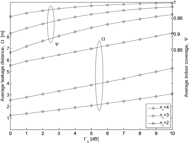
Figure 5: $\Omega$ and $\Psi$ versus $\Gamma_{\Delta}$ with shadowing , path loss exponent error ($n_{e}=3$), small number of users ($K=2$), and several non-symmetric wall penetration loss.

References

• [1] H. Claussen, L. T. W. Ho, and L. G. Samuel, β€œAn Overview of the Femtocell Concept,” Bell Labs Technical Journal, vol. 13, Issue 1, pp. 221 - 245, May 2008.
• [2] H. S. Jo, J. G. Yook, C. Mun, and J. Moon, β€œA self-organized uplink power control for cross-tier interference management in femtocell networks,” IEEE MILCOM 2008, pp. 1-6, Nov. 2008.
• [3] H.-S. Jo, C. Mun, J. Moon, and J.-G. Yook, β€œInterference Mitigation Using Uplink Power Control for Two-Tier Femtocell Networks,” IEEE Trans. Wireless Commun., vol. 8, no. 10, pp. 4906-4910, Oct. 2009.
• [4] T. Togo, I. Yoshii, and R. Kohno, β€œDynamic cell-size control according to geographical mobile distribution in a DS/CDMA cellular system,” IEEE PIMRC 1998, vol. 2, pp. 677-681, Sept. 1998.
• [5] S. H. Shin, and K. S. Kwak, β€œPower control for CDMA macro-micro cellular system,” IEEE VTC 2000 Spring, vol. 3, pp. 2133-2136, May 2000.
• [6] L. Du, J. Bigham, L. Cuthbert, C. Parini, and P. Nahi, β€œCell size and shape adjustment depending on call traffic distribution,” IEEE WCNC 2002, vol. 2, pp. 886-891, Mar. 2002.
• [7] H. Claussen, L. T. W. Ho, and L. G. Samuel, β€œSelf-optimization of coverage for femtocell deployments,” IEEE WTS 2008, pp. 278-285, Apr. 2008.
• [8] W. Jiao, P. Jiang, and Y. Ma, β€œFast handover scheme for real-Time applications in mobile WiMAX,” IEEE ICC 2007, pp. 6038-6042, June 2007.
• [9] P. Newman, β€œIn search of the All-IP mobile network,” IEEE Commun. Magazine, vol. 42, pp. S3-S8, Dec. 2004.
• [10] A. L. Garcia, Probability and random processes for electrical engineering, 2nd Edition. Addison-Wesley, 1994.
• [11] R. Hoppe, G. Wolfle, and F. M. Landstorfer, β€œMeasurement of building penetration loss and propagation models for radio transmission into buildings,” IEEE VTC 1999, Vol. 4, pp. 2298-2302, Sep. 1999.
• [12] G. Durgin, T. S. Rappaport, and H. Xu, β€œMeasurements and models for radio path loss and penetration loss In and around homes and trees at 5.85 GHz,” IEEE Trans. Commun., Vol. 46, No. 11, pp. 1484-1496, Nov. 1998.
• [13] I. Gradshteyn, I. M. Ryzhik, and A. Jeffrey, Tables of integrals, series, and products. New York: Academic, 1994.