One-quasiparticle States in the Nuclear Energy Density Functional Theory
Abstract
We study one-quasiproton excitations in the rare-earth region in the framework of the nuclear Density Functional Theory in the Skyrme-Hartree-Fock-Bogoliubov variant. The blocking prescription is implemented exactly, with the time-odd mean field fully taken into account. The equal filling approximation is compared with the exact blocking procedure. We show that both procedures are strictly equivalent when the time-odd channel is neglected, and discuss how nuclear alignment properties affect the time-odd fields. The impact of time-odd fields on calculated one-quasiproton bandhead energies is found to be rather small, of the order of 100–200 keV; hence, the equal filling approximation is sufficiently precise for most practical applications. The triaxial polarization of the core induced by the odd particle is studied. We also briefly discuss the occurrence of finite-size spin instabilities that are present in calculations for odd-mass nuclei when certain Skyrme functionals are employed.
pacs:
21.60.Jz, 21.10.Pc, 21.30.Fe, 27.70.+qI Introduction
The nuclear Density Functional Theory (dft) (Pet91) ; [Ben03] ; [Lal04] plays a central role in the quest for a microscopic and quantitative description of atomic nuclei. The energy functionals related to effective two-body density-dependent interactions are the main building blocks of the mean-field theory of the nucleus wherein the self-consistency is imposed through the Hartree-Fock-Bogoliubov (hfb) formalism. This framework has provided a consistent description of a broad range of phenomena ranging from nuclear masses to collective excitations. Over the last few years, however, with the influx of high-quality experimental data on exotic nuclei, it has become evident that the standard local functionals (e.g., extended Skyrme functionals) are too restrictive when one is aiming at detailed quantitative description and extrapolability [Sto06] ; [Ber05] ; [Zal08] ; [Kor08] . Consequently, various strategies have been devised to develop realistic nuclear energy density functionals (edf) [Ber07a] . These include: (i) the use of the density matrix expansion technique [Neg72] ; [Bog09] to relate the functional to low-momentum interactions; (ii) extending edf by adding higher-order terms in the local densities [Car08] ; and (iii) improving spin and isospin properties [Les07] ; [Sat08] ; [Sat09] ; [Mar09] . In any case, regardless of the strategy, the fine-tuning of the coupling constants of the functional to a suitably chosen set of experimental data is necessary to provide quality description [Gor09] .
When aiming at spectroscopic-quality functionals [Zal08] , the data coming from odd-mass nuclei are crucial: the energies, angular momenta, and parities of one-quasiparticle excitations provide us with basic knowledge about the underlying shell structure. Moreover, binding energies of odd- systems are instrumental for determining the magnitude of collective effects such as pairing. Theoretically, however, since nuclei with an odd number of particles have non-zero angular momentum (), i.e., they are spin-polarized, their treatment is considerably more involved as compared to the = ground-state (g.s.) configurations of doubly-even nuclei.
Mathematically, the local edf is a time-even scalar constructed from various local densities and currents related to particle and pairing density distributions [Eng75] ; [Per04] . The resulting mean field contains both time-even and time-odd terms. While the time-odd fields automatically vanish in the ground state of doubly-even nuclei, they are non-zero in configurations in which time-reversal symmetry is internally broken [Ben03] ; [Lal04] . The time-odd fields have been investigated in the context of high-spin states [Pos85wf] ; [Che92] ; [Dob95e] ; [Afa00] , Gamow-Teller excitations [Ben02] , single-particle (s.p.) spectra [Rut98] ; [Zal08] ; [Sat08] , and collective dynamics [Bar78w] ; [Dob81] ; [Mar06] ; [Hin06] . The general consensus is that they can appreciably impact the nuclear collective motion. On the other hand, our knowledge of the coupling constants characterizing individual time-odd fields is fairly limited, and the
impact of those terms on nuclear ground-states still needs to be assessed. Conversely, one can ask whether experimental data on nuclear ground states can help constrain the time-odd fields of the nuclear edf.
There have been very few systematic theoretical studies of one-quasiparticle states along isotopic or isotonic chains. Regional systematics of one-quasiparticle excitations, and their consequences on various observables in spherical and deformed nuclei, can be found in, e.g., Refs. [Ogl71w] ; [Naz90] ; [Cwi91w] ; [Cwi94a] ; [Par05] (macroscopic-microscopic approach) and Refs. [Rut98] ; [Rut99fw] ; [Cwi99] ; [Afa03] ; [Sat08] ; [Afa10] (nuclear DFT). The only global DFT study of ground state spin and parity for odd-mass nuclei is that of Bonneau et al. [Bon07] . It is to be noted, however, that most of these studies were restricted in one way or another, e.g., by assuming axial symmetry, neglecting the time-odd fields, or doing an approximate treatment of blocking. The results of Refs. [Bon07] ; [Zal08] ; [Kor08] clearly indicate that the currently used nuclear density functionals give a rather poor description of s.p. states, so it is imperative to evaluate the magnitude of the effects due to theoretical limitations and approximations.
The goal of this study is to review the description of odd-mass nuclei in the framework of the nuclear dft and assess the magnitude of time-odd polarizations through large-scale surveys. We compare various treatments of blocking, associated approximations, and resulting uncertainties. We discuss the choice of the orientation of the alignment vector, which is important for maintaining s.p. characteristics during the blocking procedure. We also assess the impact of the time-odd fields on binding energies of one-quasiparticle states and estimate the polarization due to the axial symmetry breaking in certain orbits.
This paper is organized as follows. Section II summarizes the main features of the nuclear Skyrme-dft. We pay special attention to the treatment of odd-mass nuclei through the so-called blocking approximation and the Equal Filling Approximation (efa). In Sec. III we present the details of the calculations and discuss various optimization techniques that enable large-scale calculations for odd-mass nuclei. The results are presented in Sec. IV. We first compare the efa approximation with the exact blocking prescription. We estimate the effect of the time-odd fields on one-quasiparticle states in the rare-earth region and make selected comparisons with experiment. We also comment on the finite-size instabilities related to certain energy functionals that show up when studying polarized systems. Finally, the conclusions are contained in Sec. V.
II DFT Treatment of One-Quasiparticle states
The nuclear dft in a Skyrme variant has been presented in great detail in a number of articles [Ben03] ; [Per04] ; [Sto07b] . In the following we recall only the salient features of the theory that will be needed in this study.
II.1 Representations of the Density Matrix
The cornerstone of the nuclear dft is the general one-body density operator . Two representations of the density matrix are often considered. In the coordinate representation, the s.p. space is spanned by the continuous basis of states [Ben03] ; [Bul80] ; [Dob84] ; [Dob96] . In the configuration representation, a basis of discrete states is introduced, where stands for all the s.p. quantum numbers. The choice of one particular representation depends on the context.
If is the many-body state, the non-local density matrix in coordinate representation reads:
| (1) |
where is a fermionic field operator creating a particle at position with spin projection and is the corresponding annihilation operator. The field operators can be expressed in terms of the standard fermionic creation and annihilation operators and associated with the basis (Bla86) ; (Rin80) :
| (2a) | |||
| (2b) | |||
Note that in this expression, and are matrix elements of the basis transformation : and . They are therefore complex s.p. wave functions dependent on the position vector and spin coordinate . The inverse relations are:
| (3a) | |||
| (3b) | |||
For complete bases, relations (2a-2b) and (3a-3b) allow us to express the relations between the two representations, and of the density matrix.
The density matrix (1) can be regarded as the matrix element of an operator acting in the spin space. Any such operator can be expressed in terms of the Pauli matrices and the identity matrix. This leads to a spin-scalar and a spin-vector field . These two fields are the fundamental building blocks of the nuclear dft.
II.2 Skyrme Energy Functional
The contribution to the total energy of the system coming from the Skyrme interaction reads:
| (4) |
where =0 and =1 corresponds to isoscalar and isovector components, respectively. In this paper, we do not consider proton-neutron mixing [Per04] . Using the standard notation for the local densities and currents [Eng75] ; [Per04] , the part of the energy density that depends on time-even fields can be written as:
| (5) |
while the part depending on the time-odd fields is:
| (6) |
All densities and currents entering Eqs. (5) and (6) can be related to the particle density , spin density , and their derivatives [Eng75] ; [Per04] . In the present work, we do not consider tensor interactions and therefore we set .
Below, we discuss several versions of the functional, depending on how the time-odd coupling constants are determined:
-
•
Native version, which corresponds to all time-odd coupling constants being determined by the underlying Skyrme interaction [Per04] .
- •
-
•
Landau version, which is based on the gauge version where the subset of time-odd coupling constants and are reset through the Landau parameters [Ben02] :
(7) where , and, additionally, for . Since the Landau prescription only sets , the gauge condition is broken since anymore.
-
•
Time-even version, in which all time-odd coupling constants in Eq. (6) are set equal to zero.
II.3 HFB Method
In the hfb theory, pairing correlations enter through the pairing tensor defined in coordinate representation as:
| (8) |
(From a practical point of view, it is sometimes more advantageous to use the pairing density [Dob84] ; [Dob96] .)
The starting point of the hfb theory is to assume that the ground-state of an even-even nucleus is a vacuum for quasiparticle operators . The latter are obtained from single-particle operators associated with the single-particle basis states by the Bogoliubov transformation:
| (9a) | |||
| (9b) | |||
The matrices and are obtained from the hfb equations:
| (10) |
where is the chemical potential, is the Hartree-Fock (hf) potential and the pairing potential. (From a practical point of view, it is sometimes more advantageous to use the pairing potential [Dob84] ; [Dob96] .) The form of the hfb equations in coordinate space can be found in Refs. [Dob84] ; [Dob96] .
The density matrix and pairing tensor can be written as:
| (11a) | |||
| (11b) | |||
The coordinate representation of the Bogoliubov transformation,
| (12a) | |||
| (12b) | |||
can be expressed through lower and upper components of the quasi-particle (q.p.) wave functions:
| (13a) | |||
| (13b) | |||
Finally, the density matrix and pairing tensor in coordinate space are:
| (14a) | |||
| (14b) | |||
It is assumed here that the q.p. continuum with has been discretized and all q.p. states with energy lower than some cut-off energy are retained (see discussion in Ref. [Dob84] ).
II.4 The Blocking Prescription and the Equal Filling Approximation
In the hfb theory, the ground-state of an odd nucleus is a one quasiparticle excitation with respect to the q.p. vacuum. In the configuration representation, the corresponding density matrix and pairing tensor are [Ban74] ; [Fae80] ; [Ber09] ; [Per08] :
| (15a) | |||
| (15b) | |||
In practice, one must adopt a prescription to be able to determine, at each iteration, the index of the quasiparticle state to be blocked [Hee95] . In the present study, this has been done according to the recipe described in Ref. [Dob09d] . In the first step, the mean field Hamiltonian is diagonalized:
| (16) |
Since in this work parity and -signature are assumed to be self-consistent symmetries, every s.p. level is uniquely identified by its position in a given parity and -signature block. This unique identification allows to pin down the configuration of the blocking candidate . To connect the s.p. state with a quasiparticle state to be blocked, we calculate at each iteration the overlap between and both the upper component and the time-reversed lower component of quasiparticle states around the Fermi level [Dob09d] . The largest overlap in this set defines the index of the quasiparticle state to be blocked. In the beginning of the iterative process, s.p. states of a neighboring even-even nucleus are taken.
Within the efa, the states and its time-reversal partner enter the density matrix and pairing tensor with the same weights, which ensures time-reversal symmetry and thereby degeneracy of and [Per08] :
| (17a) | ||||
| (17b) | ||||
The hfb equations are then solved by replacing (, ) with (, ). For the justification of the efa ansatz by means of statistical density operators and for detailed discussion of the procedure involved, we refer the reader to Refs. [Per08] ; [Per07] .
In this work we point to another possible justification of the efa. We first notice that the time-even parts of the blocked density matrices given by Eqs. (15a) and (15b) are identical to the time-even parts of the density matrices in efa, Eqs. (17a) and (17b). Therefore, all time-even densities in Eq. (5) are exactly the same in both variants. Consequently, in the blocking and efa approximations, the time-even part of the functional (Sec. II.2) yields exactly the same self-consistent solution. This allows us to reinterpret efa density matrices as those corresponding to the time-even functional in which the time-odd polarizations exerted by the odd particle are dynamically switched off. Of course, the blocking prescription and efa give exactly the same average values of all time-even observables (e.g., radii and multipole moments) but differ in the average values of time-odd observables (e.g., spin alignments and magnetic moments).
II.5 Blocking, Alignments, and Symmetries
Although for the functionals restricted to time-even fields (or within efa) the time-reversed q.p states and are exactly degenerate, this is not true any more in the general case. Here, the blocking prescription does depend on which of these two states, or which linear combination thereof, is used in Eqs. (15a) and (15b). In order to discuss this point, we introduce here the notion of an “alispin”, which pertains to the unitary mixing of states and . This is in complete analogy with the standard notion of the isospin, which involves the unitary mixing of proton and neutron states.
An alivector is defined as a set of two complex numbers and ():
| (18) |
which corresponds to the linear combination of states and : . Alivectors reside in SU(2) space; therefore the alirotation by an angle is defined as:
| (19) |
where the alivectors of Pauli matrices are denoted by , and denotes the scalar product of alivectors. To recall that the alirotation pertains to a single pair of states, we use superscripts throughout.
The blocked density matrix Eq. (15a) corresponding to the state reads:
| (20) |
If time-reversal symmetry is conserved, the different blocks of the Bogoliubov matrices are related:
| (21) |
and . These relations lead to:
| (22) |
or, equivalently
| (23) |
Therefore, in this limit, the exact blocking density matrix becomes independent of the coefficients of the mixing, i.e., it is an aliscalar. Since
| (24) |
the efa density matrix also coincides with the exact blocking density matrix; hence, it is an aliscalar as well.
In the general case where time-reversal symmetry is not dynamically conserved, however, the blocking density matrix is not aliscalar and the energy of the system may change as a function of the mixing coefficients . To analyze what are the consequences of blocking different alirotated states , we introduce the (real) alignment vector and the (complex) decoupling vector [Olb06] . Together, they form the matrix elements of the alignment vector-alivector :
| (25) |
Expanding this operator (acting on SU(2) alistates) in the basis of Pauli matrices, we find:
| (26a) | ||||
| (26b) | ||||
| (26c) | ||||
where indices enumerate the components of alivectors. From these considerations it follows that the alignment vector-alivector , which corresponds to the alirotated pair (19), is obtained by:
| (27) |
where are the standard spin-1 matrices (Var88) , which are generators of rotation in the vector representation. This shows that the concept of alirotation (equivalent to changing the mixing of the blocked state) translates into a change in the alignment of the system.
To illustrate how this works, let us examine the special case where the states and are eigenstates of the signature operator. Since:
| (28) |
we can express the states and in terms of -eigenstates:
| (29) |
which corresponds to the rotation of the system by the Euler angles . Consequently, the alivector is the vector alirotated by the angles . Since (i) the blocked density matrix is not an aliscalar, and (ii) alirotations are induced by rotations of the coordinate system or, equivalently, a change of the symmetry operators used to label s.p. and q.p. states, we must conclude that the blocked density matrix may depend on the choice of the symmetry operators that commute with the Hamiltonian111Note that, in the particular case where the alivector is built from the eigenstates and of , the alirotation by is equivalent to the symmetry, and therefore leaves the system invariant. This operation corresponds to . Therefore, in this particular case, blocking state or state gives exactly the same energy, even though time-reversal symmetry is internally broken and the q.p. spectra do not exhibit the Kramers degeneracy..
More generally, since all alignment properties of the system are embedded in the vector-alivector operator , we also see that the alirotation of states and corresponds to hfb states having different alignment vectors. Therefore, the latter can be used to tag blocked states. This is a very convenient method, which can be applied not only for the time-even version of the functional when the quasiparticle states and are degenerate, but also in the case of internally broken time-reversal symmetry. The key to our considerations of blocked states is the realization that blocking must depend on the orientation of the alignment vector with respect to the principal axes of the mass distribution. Therefore, the only rigorous way to proceed would be for each quasiparticle excitation to vary the orientation of the alignment vector with respect to the principal axes of the system, and retain the solution with the lowest energy [Olb04] . We give in Sec. IV.2.3 a pedagogical illustration of such anisotropy of blocking.
In many practical applications, however, one chooses a fixed direction of alignment dictated by practical considerations. In particular, the identification of blocked single-particle states and quasiparticle states is most conveniently carried out through the set of conserved quantum numbers characteristic of the problem. In all calculations performed in this work, nuclei are either axially deformed or nearly axial, and they conserve reflection symmetry. The corresponding symmetry group is ; hence, signature and parity are good quantum numbers. In hfodd signature is defined with respect to the -axis of the reference frame [Dob04b] . In this way, the alignment vector is restricted to having only the -component. To realize the three possible alignments of the angular momentum along the principal axes, it is sufficient to orient the longest, shortest, or intermediate axis along the -axis. Since in most cases, the configurations analyzed in this study are axial, only two orientations suffice. We show in Sec. III.1 below how to implement such a scenario.
Equivalently, one could work with a good -simplex basis such as in Ref. [Gir83] . In that case, the default alignment is along the -axis, but results still depend on the orientation of the body. It is only by allowing the alignment vector to cover the full solid angle that physical properties of the system would not depend on the choice of the basis used to describe the odd nucleus.
III Method of Calculation and Optimization Techniques
This section briefly describes the dft solvers used in this work and discusses the choice of parameters entering our calculations. We also outline various optimization techniques that have been implemented by us to carry out large-scale dft calculations for one-quasiparticle states on leadership class computers.
III.1 Numerical Parameters
All calculations in this work are performed with the dft solvers hfbtho [Sto05] and hfodd [Dob04b] ; [Dob05] ; [Dob09d] . Both codes solve the Skyrme hfb problem in the configuration space by means of the Harmonic Oscillator (ho) expansion technique. In hfbtho, the cylindrical ho basis is used, and both axial and time-reversal symmetries are imposed. This implies that the efa must be used for blocking calculations. The 3D solver hfodd employs the Cartesian ho basis and is symmetry-unrestricted. This unique feature of hfodd makes it a tool of choice for our study, since in the polarized nuclear configurations many self-consistent symmetries are usually broken. The blocking prescription is implemented exactly in hfodd with all the time-odd fields taken into account. Both codes have been benchmarked against one another and they yield the same results within a few eV for spherical or axially deformed even-even nuclei [Dob04a] .
As already mentioned, all nuclei considered in this work are either axial or slightly triaxial, as well as reflection-symmetric. Therefore -signature and parity are conserved and used in hfodd to tag q.p. and single-particle states. However, this implies that the total alignment is confined to the -axis. Since the latter is not the quantization axis, one can not easily associate the single-particle spin with the expectation value of the angular momentum: the situation is analogous to the collective rotation in high-spin physics. For the sake of identification of deformed Nilsson orbitals, it is convenient, however, to reintroduce as a (nearly) good quantum number by orienting the angular momentum along the -axis; the resulting alignment properties correspond to the limit of non-collective rotation.
To this end, we need to associate the quantization axis with the symmetry axis of the nucleus. This can be achieved via a Euler rotation of the body-fixed frame (by , , ) or by imposing constraints on the expectation values of the quadrupole tensor . After testing these two options, we choose the Euler rotation: calculations for even-even nuclei are performed in the standard -signature mode, then solutions are Euler-rotated and used to warm-start calculations for odd-nuclei. In this way, the Nilsson quantum number is computed from the expectation value of . This technique turns out to be both stable and fast. Note that the energies of a given blocked state in the Euler-rotated case and original orientation are different, as discussed in Sec. II.5. Only a complete survey of all possible orientations of the alignment vector, which would be a major computational endeavour, could pin down the correct orientation.
As is well known, calculations for deformed nuclei converge faster if the eigenstates are expanded on a stretched basis that follows the geometry of the nuclear density. Unfortunately, the stretched basis is not compatible with the Euler-rotation of the nucleus in space in hfodd. For that reason, all calculations presented in this work have been carried out in a full spherical basis of =14 oscillator shells (the number of basis states is = 680). This choice guarantees stability of results for the relatively modest deformations considered in this study. The oscillator frequency was fixed at [Dob97] for MeV.
In this work, we use three commonly used Skyrme parametrizations: SIII [Bei75] , SkP [Dob84] , and SLy4 [Cha98] . In the pairing channel, we employ the density-dependent delta interaction in the mixed variant [Dob02c] :
| (30) |
where fm-1 and is the pairing strength (identical for protons and neutrons). Note that the use of such a zero-range interaction requires us to introduce a renormalization (or regularization) procedure to avoid non-physical divergences [Bul02] ; [Bor06fw] . We employ the standard value =60 MeV.
For each Skyrme edf, the pairing strength has been adjusted to reproduce the experimental proton odd-even mass difference in the deformed nucleus 162Dy, MeV. This choice has been motivated by the findings of Ref. [Ber09a] that by adjusting to experimental data for a spherical semi-magic nucleus one underestimates pairing correlations in deformed systems having lower single-particle level density around the Fermi surface. Moreover, by considering the proton pairing gap, one effectively takes into account the Coulomb contribution to pairing [Les08] . The pairing strengths used in this work are MeV, MeV, and MeV for SLy4, SIII, and SkP, respectively. In Sec.IV.5, we also consider SkO, MeV, and SkM*, MeV.
III.2 Parallelization and Optimization
The advent of Teraflop and Petaflop supercomputers enables large-scale surveys with symmetry-unrestricted dft solvers. To optimize resources, however, optimization of the production codes is required. Starting from the original published versions of hfodd and hfbtho, we made a number of improvements. First of all, a parallel interface using the standard Message Passing Interface (MPI) has been constructed to allow the automated distribution of calculations over several computing cores. Let us note that the standard nuclear dft calculations are “embarrassingly parallel”. Indeed, solving the hfb equations for one nuclear configuration usually does not exceed a few hours on a standard desktop computer. Therefore, each computing core of a massively parallel system can process a single hfb task corresponding to a particular nucleonic configuration. Only in the limit of very large ho bases, or for dft solvers constructed in the coordinate space, does the parallelization of the solvers become necessary. The advantage of using massively parallel architectures is that simultaneous calculations of hundreds or thousands of different many-body configurations are possible in a very reasonable time. Such a strategy makes it possible to extract systematic trends, use standard statistical analysis toolboxes, and ultimately develop nuclear edfs of spectroscopic quality.
The scaling of a dft problem with the number of processors also implies that a simple master-slave parallel architecture is sufficient for most applications, and this solution is adopted here. All calculations in this study were performed on the Cray XT3/XT4 Jaguar supercomputer at the National Center for Computational Science at the Oak Ridge National Laboratory and on the Cray XT3 Franklin supercomputer at the National Energy Research Scientific Computing Center at the Lawrence Berkeley National Laboratory. Typical production runs have involved from 8,000 to 12,000 computing cores per run, and the typical calculation time was about 2 hours.
The hfb equations represent a coupled system of non-linear equations for nucleonic densities. The non-linearity enters through the dependence of the mean fields on densities (self-consistency). In order to diminish the number of iterations required to attain a given precision, we employ the modified Broyden method [Joh88] ; [Bar08] . The method is based on the observation that the convergence of the hfb process stops when the characteristic variables in the problem, for example the density , do not change any more from one iteration to the next: . In other words, the hfb equations can be viewed as a fixed-point problem, and iterations can therefore be optimized by employing a quasi-Newton method. It was shown that the computational cost (in units of number of iterations) could be reduced substantially, by a factor of 3 to 4. Our particular implementation of the modified Broyden method was described in Ref. [Bar08] .
As mentioned earlier, hfodd solves the hfb problem by expanding eigenvectors in the Cartesian ho basis. In terms of speed, one of the major bottlenecks in hfodd is the diagonalization of the hfb matrix. The latter is carried out with the subroutine zheevr of the lapack library. We found that a significant gain in terms of speed, up to 30-40% for large ho bases with, e.g., =20 shells, could be obtained by using machine-specific implementations of the blas and lapack libraries, such as atlas.
III.3 Massively Parallel Calculations: Convergence Improvements
Based on the experience gained in self-consistent calculations for odd- nuclei, it appears that calculations involving blocking are always less stable than those performed for even-even nuclei. Apart from the specific issue related to finite-size instabilities addressed in Sec. IV.5 below, these numerical instabilities are related to the need to select, at each iteration, the blocked q.p. state. The blocking procedure is outlined in Sec. II.4 and the detailed justification can be found in, e.g., Ref. [Hee95] . The selection method implies that the blocked q.p. state may change from one iteration to the next, in particular at the beginning of the calculation. This numerical noise is the price to pay for the full self-consistency, and it explains why small differences in the initial conditions can actually affect the convergence process.
When only a few nuclei are considered, and a small number of blocked configurations near the ground-state is calculated, one can often find ways to converge calculations, such as: (i) changing the linear-mixing parameter of the self-consistent scheme; (ii) starting from the unblocked fully-paired state corresponding to an odd average particle number (false vacuum) [Dug01a] ; (iii) starting from the even-even nucleus with one more particle for a particle-like blocked state and with one particle less for a hole-like blocked state, as implemented in Ref. [Hee95] (we also used this method in our calculation); (iv) using different values of the linear-mixing parameter for time-even, time-odd, and/or pairing fields. Whenever a blocking calculation fails to converge, one may repeat it by using one or several of these tricks until a converged result is obtained. This is what was done in previous studies involving self-consistent calculations, and it was possible, because these studies were focused on ground-state properties and only a minimum number of different configurations was considered.
| Exact State | ) | |||||||
|---|---|---|---|---|---|---|---|---|
| Blocking | efa | Exact | efa | Exact | efa | Exact | efa | Exact |
| (MeV) | ||||||||
| (MeV) | ||||||||
| (MeV) | ||||||||
| (MeV) | ||||||||
| r.m.s (fm) | ||||||||
| (b) | ||||||||
| (MeV) | ||||||||
| (MeV) | ||||||||
| (MeV) | ||||||||
| (MeV) | ||||||||
| (MeV) | ||||||||
| () | ||||||||
| () | ||||||||
In our case, however, we consider thousands of configurations and such a trial-and-error scheme, however helpful, is simply impossible to implement. Instead, we have resorted to a simple trick; namely, since the initial conditions do matter, we artificially generate slightly different initial conditions for the two signature partners that converge to practically the same result.
The main idea here consists in adding a tiny rotational frequency of about =0.001 MeV to break the degeneracy of signature configurations. This improves the convergence rate at the price of an insignificant numerical error of about 1–2 keV, on average. We illustrate this fact by two specific examples of blocked states in 163Tb (native version, non-collective orientation) with different alignments. For the blocked state [411]1/2, at =0 the total energy equals 1322.279268 MeV, while for =+0.001 and 0.001 MeV the total energies read 1322.279480 MeV () and 1322.279188 MeV (), respectively. Similarly, for the blocked state [404]7/2, the three corresponding energies are: 1321.725322 MeV, 1321.725538 MeV (), and 1321.726010 MeV (). To make our point, we deliberately show these energies with far too many digits than it is physically relevant. In these particular two examples, the numerical precision of the calculation is 10 eV, which is exceptionally good for odd nuclei. Therefore, the noted differences can only be attributed to the effect of the cranking term. Without this term, by blocking states and one always obtains exactly the same hfb energy, , because the full Skyrme functional is time-even.
IV Results
This section presents a number of Skyrme-hfb results for odd-mass nuclei. We begin by giving a detailed numerical comparison of the efa with the exact blocking prescription in the limit of conserved time-reversal symmetry. The impact of time-odd fields on the quasiparticle spectrum in the rare-earth region is shown in Sec. IV.2 with the native, gauge, and Landau versions of SIII, SkP, and SLy4 functionals. The role of the nuclear alignment vector on physical observables is also studied. Results of calculations are compared with selected experimental data in Sec. IV.3. The triaxial polarization induced by a blocked quasiparticle is discussed in Sec. IV.4. Finally, Sec. IV.5 mentions the problem of the intrinsic instability of certain Skyrme functionals that appear when time-odd terms are included.
IV.1 Validation of the EFA Approximation
To demonstrate the numerical precision of our calculations, Table 1 shows the results for four one-quasineutron states in 121Sn obtained with hfbtho (efa) and hfodd (exact blocking). They are selected based on the mean-field spectrum (16) of 120Sn. For the sake of this comparison, the time-odd fields in hfodd have been switched off, thereby enforcing the regime where the exact blocking procedure is strictly equivalent to the efa, see Sec. II.4. Indeed, the obtained numerical differences between the efa and exact blocking are extremely small, less than 1 keV for the four different cases shown in Table 1. This can be entirely attributed to various implementations adopted differently in the two codes such as the method of computing the Coulomb potential, etc. The even-even core 120Sn is spherical in its ground state. The quasiparticle blocking slightly polarizes the nuclear shape inducing small quadrupole deformations for some configurations.
Although the time-even observables obtained within the efa and exact-blocking are strictly identical if the time-odd fields are disregarded, this is not true for time-odd observables. In Table 1, this is illustrated by the values of alignments of the blocked quasiparticles aligned parallel () or perpendicular () to the symmetry axis. Of course, without time-odd fields, the direction of alignment does not influence the time-even observables.
| efa (hfbtho) | Exact (hfodd) | |||
| Blocked State | (b) | (MeV) | (b) | (MeV) |
| 18.514 | 1323.495 | 18.514 | 1323.495 | |
| 17.759 | 1322.648 | 17.759 | 1322.647 | |
| 18.554 | 1322.415 | 18.555 | 1322.414 | |
| 18.384 | 1322.322 | 18.384 | 1322.322 | |
| 18.654 | 1322.151 | 18.654 | 1322.151 | |
| 20.138 | 1321.771 | 20.136 | 1321.773 | |
| 17.291 | 1321.357 | 17.290 | 1321.357 | |
| 17.034 | 1320.762 | 17.032 | 1320.762 | |
| 17.766 | 1320.090 | 17.767 | 1320.090 | |
| 19.266 | 1319.851 | 19.266 | 1319.851 | |
Rare-earth nuclei provide an excellent testing ground for studies of deformed Nilsson orbits. Many of those nuclei are well-deformed, near-axial rotors and the deformed mean field theory is particularly suitable to describe their structural properties. Table 2 shows a comparison for several one-quasiproton configurations in a well deformed odd-proton nucleus 163Tb. In hfbtho, the determination of a blocking candidate was made using the mean-field spectrum (16) of the even-even core 162Dy. In the case of hfodd, to improve speed and stability of the iterative process [Hee95] , blocking candidates of a particle character (above the proton Fermi level of 162Dy) were selected from the mean-field spectrum of 164Dy while hole-like levels were selected from that of 162Dy. Of course, the final results do not depend on which particular even-even nucleus has been used as a core.
The results shown in Table 2 show again that without time-odd fields, the full blocking procedure is equivalent to the efa. It is worth noting that the difference on the total energy is less than 1 keV for all of the excited states, and less than 0.002 b for the quadrupole moments, regardless of the quadrupole polarization exerted by a blocked state.
IV.2 Effect of Time-Odd Fields
This section illustrates the effect of the various prescriptions for the time-odd channel (6) of the functionals. Calculations were performed for all odd-proton nuclei with 6375 and 78104. For each of them, 14 non-degenerate blocked configurations around the Fermi level have been considered. Altogether, 3,822 independent one-quasiproton states were studied.
IV.2.1 Native Functionals
Table 3 displays results for one-quasiproton states in 163Tb in the time-even, native, gauge, and Landau variants of calculations. The alignment and elongation axes coincide with the -axis of the reference frame. The time-even energies are shown in the absolute scale. For other variants, shown are displacements with respect to the time-even case:
| (31) |
In the particular example shown in Table 3, the maximum shift in one-quasiparticle levels due to the time-odd terms of the native functional is 127 keV. This is consistent with the earlier results of Refs. [Dug01a] ; [Dug01b] and overall smaller than in the relativistic mean field approach, where time-odd polarization corrections seem to range from only a few dozen of keV in deformed actinides up to half a MeV in light nuclei [Afa03] ; [Afa10] .
| Blocked State | Time-even | Native | Gauge | Landau |
|---|---|---|---|---|
| 1323.495 | 0.075 | +0.042 | 0.125 | |
| 1322.647 | 0.052 | +0.029 | 0.105 | |
| 1322.410 | 0.060 | +0.039 | 0.080 | |
| 1322.322 | 0.043 | +0.040 | 0.118 | |
| 1322.151 | 0.048 | +0.062 | 0.085 | |
| 1321.773 | 0.007 | +0.055 | 0.075 | |
| 1321.357 | 0.047 | +0.036 | 0.107 | |
| 1320.762 | 0.037 | +0.017 | 0.161 | |
| 1320.090 | 0.127 | +0.018 | 0.231 | |
| 1319.851 | 0.121 | +0.036 | 0.150 |
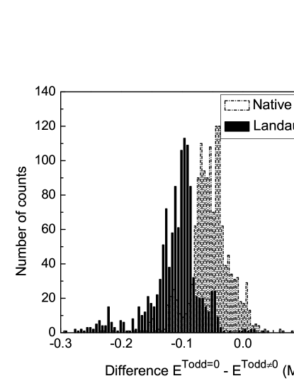
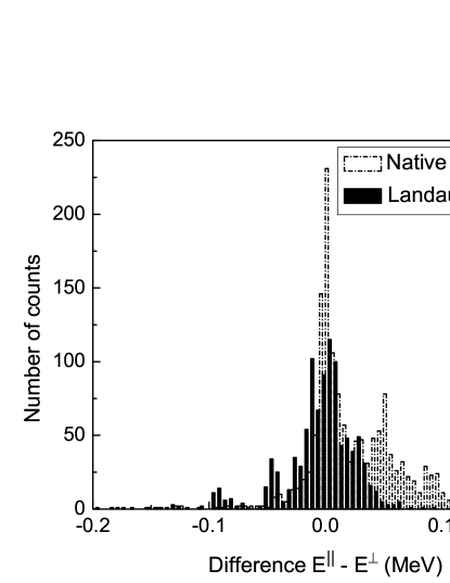
The overall impact of the time-odd fields on the energy of one-quasiproton states in the deformed rare-earth nuclei is summarized in Fig. 1 which shows the distribution of (31) for SIII, SkP, and SLy4 edfs. When native functionals are used, the total number of converged cases is 1,404 (524 for SIII, 443 for SkP, and 437 for SLy4). The average value of is –50 keV with a standard deviation of 42 keV.
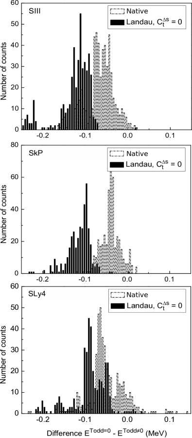
The magnitude of the odd-time effect depends on the choice of the edf. To illustrate this point, Fig. 2 displays the distribution of for individual functionals. Focusing in this section on the native functionals (dot-dashed open bins), it is seen that the largest time-odd effect is predicted for SIII, which also shows an appreciable spread in values (configuration dependent). On the other hand, for the SkP parametrization the distribution of is fairly narrow, centered around –40 keV.
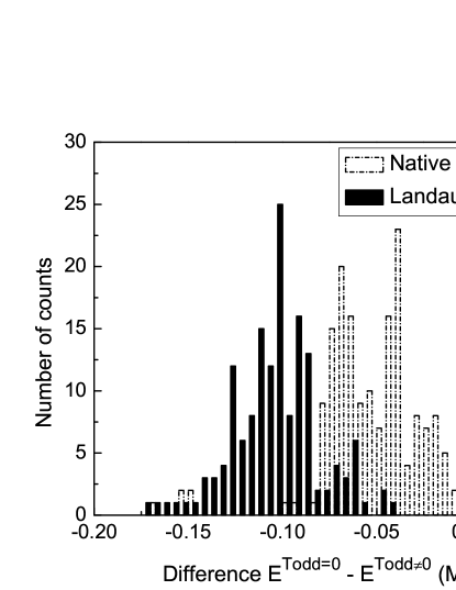
By construction, Figs. 1 and 2 contain contributions from g.s. configurations and from nearly-lying excited states. Since g.s values are of particular importance as they impact mass predictions, Fig. 3 shows for g.s. configurations only. The average value of the g.s. time-odd displacement is only 50 keV. Most of the few cases with keV correspond in fact to a collapse of pairing correlations in one of the 2 sets of calculations. It may be worth noting that the most recent hfb mass formula based on the Skyrme BSk17 parametrization yields a r.m.s deviation of 581 keV [Gor09] . The uncertainty associated with neglecting the time-odd fields appears, therefore, to be smaller by an order of magnitude.
In order to discuss the configuration dependence of the time-odd displacement, it is instructive to identify the s.p. orbits of interest. To this end, Fig. 4 shows the evolution of the proton s.p. energies, defined as the eigenvalues of the mean field operator (16), in the nucleus 164Dy calculated with SLy4 as a function of the axial quadrupole deformation . This Nilsson diagram has been obtained by carrying out a set of constrained hfb calculations along a one-dimensional path.
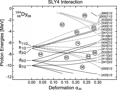
Although the values of are usually small, there are a few cases where the displacement can amount to more than 100 keV. A detailed analysis of the blocked configurations for all three interactions shows that the largest deviations correspond essentially to the [420]1/2, [404]9/2, [400]1/2, and [505]11/2 Nilsson orbitals. It is interesting to note that the value of the s.p. angular momentum does not seem to be crucial, since these states can be associated with both low and high- spherical shells. In deformed rare-earth nuclei, equilibrium deformations are . As seen in Fig. 4, in this deformation range, the orbital [420]1/2 is a deep-hole state while [404]9/2, [400]1/2, and [505]11/2 are highly excited particle states. All these one-quasiproton excitations are strongly oblate-driving. A similar result has also been obtained for SLy4 and SkP.
IV.2.2 Landau functionals
Traditionally, only the time-even channel of Skyrme functionals has been adjusted to selected experimental data. That is, the time-odd channel has usually not been constrained. This is illustrated by the broad spread of the values of the isoscalar Landau parameters and of the standard Skyrme functionals [Ben02] ; [Zdu05] . In [Ben02] , a careful study of Gamow-Teller resonances within the Skyrme EDF theory yielded a set of ‘optimal’ Landau parameters that could be used to fix some of the coupling constants of the time-odd channel of the functional (namely the and ).
As seen in Table 3, the time-odd polarization in the Landau variant is greater than in the native variant, with the largest shift growing to 231 keV. The time-odd shifts in the gauge variant are generally smaller than for the native and Landau parameterizations. They also have opposite sign (time-odd polarization in the gauge variant decreases the binding energy while it is repulsive in native and Landau variants).
The solid-filled bins in Figs. 1–3 show for Landau-corrected functionals. The effect of this correction is significant, as it shifts the centroid of most histograms by about 100 keV for SIII and SkP and 50 keV for SLy4. When only ground-states are considered, the overall shift is of the order of 50 keV.
To finish this section, let us recall that setting was motivated in [Ben02] to reproduce the energy and strength of the GT resonance, although different conclusions about the role of this term were obtained later in [Fra07] . In any case, the isoscalar channel governed by the term is not constrained by GT resonances, and in Refs. [Ben02] ; [Zdu05] ; [Sat08] ; [Zal08] these terms are set to zero essentially to ensure the stability of the calculation. We briefly discuss this point in Sec. IV.5.
IV.2.3 Alignments and Choice of the Quantization Axis
As discussed in Sec. II.5, one of the characteristic features of the treatment of odd nuclei in the blocking approximation is the dependence of time-odd densities on the orientation of the alignment vector with respect to the principal axes or, equivalently, the choice of the self-consistent symmetries and quantization axis. To measure this effect, we performed two sets of calculations. The first variant () corresponds to the alignment vector aligned along the -axis, and the shape symmetry axis aligned along the -axis. In the terminology of the cranking model, this case represents “collective rotation” perpendicular to the symmetry axis. In the second variant (), the nucleus is rotated by 90, as described in Sec. III.1, so that the alignment and symmetry axes coincide with the -axis (“non-collective rotation”).
Note that in both situations -signature and parity are conserved: the identification of blocking configurations via the position of the blocked state in a given signature/parity block hence provides a very robust way of tracking configurations before and after the Euler-rotation, as it is independent of the changes in other spatial characteristics of the quasi-particle wave-functions. As mentioned in Sec. III.1, the original Nilsson label of a q.p. state can be easily recovered in the non-collective orientation by simply exchanging the roles of the and axis in their computation.
In Fig. 5 we show the distribution of differences for the 3,822 cases presented in the previous section (only those well converged are included in the plot). It is seen that the time-odd polarization due to the orientation of qp alignment gives an appreciable contribution to the time-odd shift, with the average value of being about 50 keV in the native variant. The orientation effect seems to be weaker for Landau functionals. While the energy shift depends on the actual configuration, the total energy in the collective rotation scenario () is overall lower than in the non-collective one () when native functionals are used.
IV.3 Experimental Odd-proton Spectra
In well-deformed nuclei, one quasiparticle states can be related to the rotational band-head configurations (Boh75) . In rare-earth nuclei, rich systematics of experimental data exist, and most importantly, the customary assignments of Nilsson labels are available [Naz90] ; (ensdf) . Although these labels are approximate, they facilitate the comparison between theory and experiment.
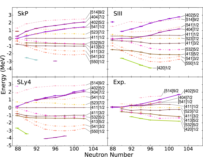
In Fig. 6 we show the one-quasiproton spectra for the Ho (=67) isotopic chain predicted with SkP (upper-left panel), SIII (lower-left panel), and SLy4 (lower-right panel) functionals in the native variant. They are compared to experimental data. We follow the convention of Refs. [Nie75] ; [Naz90] , whereby the hole-like excitations are plotted below zero (representing the g.s. configuration) while the particle-like states are plotted above zero.
The comparison with experiment suggests that the functional parametrizations employed in our work are not of spectroscopic quality for deformed nuclei. While the general deformation trends are reproduced and most of the orbitals found experimentally are indeed predicted to appear around the Fermi level, the quantitative agreement with the data is not particularly impressive. For example, the SLy4 parametrization fails to reproduce the observed [523]7/2 g.s. of Ho isotopes; this state is predicted to lie 300–500 keV above the calculated [411]1/2 ground state. Surprisingly, the oldest Skyrme parametrization SIII gives the best reproduction of experimental band heads. The result of Fig. 6 is consistent with the conclusions of Ref. [Bon07] ; they found that the agreement of both spin and parity in the self-consistent models reaches about 40% for well-deformed nuclei regardless of the Skyrme force used.
The three functionals used here have different isoscalar effective masses, =1, 0.707, and 0.7 for SkP, SIII, and SLy4, respectively. The effect of on shell structure is complex [Kor08] ; among others, it impacts the density of states around the Fermi level. As seen in Fig. 6, the average level density obtained with SkP is indeed close to the experimental one. However, this does not necessarily mean that the spectroscopic properties are better described with this interaction: just as for SLy4, the ground-state is incorrectly assigned to the [411]1/2 orbital for all isotopes.
There are, indeed, many factors that may impact the order of one-quasiparticle states. The recent analysis of spherical s.p. shell structure [Kor08] has demonstrated that the isoscalar coupling constants in edf have a large impact on the position of s.p. energies and spin-orbit splitting. It was also shown that the role of the effective-mass coupling constant cannot be reduced to merely changing the overall density of states. In fact, effective mass significantly influences relative positions of single-particle levels, including the splitting of spin-orbit partners.
IV.4 Triaxial Shape Polarization
Triaxial deformations of nuclear shape are enhanced at high spins (Szy83) ; [Fra00] . One spectacular example is the nuclear wobbling motion, which is caused by the fast rotation of triaxially-deformed nuclei (Boh75) ; [Sho09] ; [Ode01w] ; [Jen02w] . The phenomena of nuclear chirality is also tightly related to axial asymmetry [Fra97] ; [Olb04] ; [QiZ09] . Recently, a systematic study of ground-state nuclear shapes in the framework of the macroscopic-microscopic model has also pointed to regions of triaxial instability in the nuclear chart [Mol06] .
In the deformed rare-earth region that we consider in this work, the blocking of a quasiparticle built on intruder configurations has a strong -driving effect [Fra83] ; [Ham83w] ; [Abe90] ; [Mat07] . Most of the studies of this phenomenon are so far confined to high-spin states. Our calculations offer the opportunity to assess the degree of triaxiality in the g.s. configurations associated with weakly spin-polarized states.
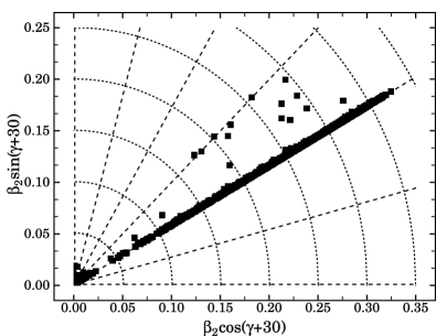
The calculated equilibrium deformations of one quasi-proton configurations considered in our survey are displayed in Fig. 7. Time-odd terms are set to zero, so that results can be compared with the time-even calculations performed with hfbtho that define the axial reference point. As apparent in Fig. 7, for the majority of configurations, triaxiality is very small, with deformation typically less than 1.
| Z | N | E∗ (MeV) | (deg) | (keV) | |
|---|---|---|---|---|---|
| 69 | 90 | 1.506 | 0.21 | 7.7 | -191 |
| 69 | 92 | 2.070 | 0.25 | 6.7 | -187 |
| 69 | 94 | 2.471 | 0.28 | 5.9 | -191 |
| 69 | 96 | 2.745 | 0.29 | 5.4 | -184 |
| 69 | 98 | 2.955 | 0.30 | 4.0 | -124 |
| 71 | 86 | 0.232 | 0.13 | 19.6 | -233 |
| 71 | 88 | 0.647 | 0.17 | 11.8 | -214 |
| 71 | 90 | 1.106 | 0.20 | 8.9 | -195 |
| 73 | 88 | 0.442 | 0.16 | 8.1 | -203 |
| 73 | 90 | 0.717 | 0.18 | 8.9 | -205 |
Only a few highly excited states are characterized by a sizeable triaxial polarization: One such example is the state [402]3/2, which originates from the spherical d3/2 orbital from the major shell and is pushed up into the major shell because of deformation. In Table 4 we show the equilibrium deformations calculated with SLy4 for this specific configuration in a number of isotopes. The excitation energies of [402]3/2 range from 0.2 to 3 MeV. On average, the net energy gain induced by the triaxial polarization of the core is of the order of 200 keV in this extreme case.
As indicated, the results presented in Fig. 7 have been obtained by setting all time-odd fields to zero. When this constraint is released, g.s. configurations remain overwhelmingly axial, independently of the orientation of the alignment vector, cf. discussion in Sec. II.5. However, we do observe that in the collective orientation limit, low- intruder states such as [541]1/2 (from h9/2) and [550]1/2 (from h11/2), or high- intruder states such as [505]11/2 (from h11/2), seem slightly more unstable against -polarization than in the non-collective situation.

This overall axial stability is illustrated in Fig. 8, where the distributions of the angles for well-deformed odd-proton states in the rare-earth nuclei are plotted. For better legibility of the figure, the very rare pronounced triaxial cases with have been omitted - they have been discussed above, and so have the many near-axial states with . In the lower panel corresponding to the collective orientation, the few points beyond correspond to the -driving orbitals. If the rotational frequency is increased (cranking), we find that the degree of triaxiality increases accordingly [Fra83] ; [Ham83] ; [Abe90] .
IV.5 Finite-size Instabilities of Band-head Calculations
It has been shown that some parametrizations of the Skyrme energy functional could be prone to finite size instabilities [Bla76] ; [Cau80a] ; [Les06] . In particular, the time-even and time-odd terms could, in some cases, lead to divergences of the hfb iterative procedure. The size of these instabilities depends on a number of factors such as the edf parametrization, particle number, and specific implementation of the dft solver. The detailed analysis of edf instabilities performed in [Les06] has been based on the rpa response function approach of Ref. (Fet71) implemented to Skyrme functionals [Gar92b] ; [Mar06a] . Results were reported in 40Ca and 56Ni for the SkP and SLy5 parametrizations.
Finite-size instabilities governed by terms are amplified in polarized systems such as odd-mass nuclei. Indeed, these terms are only active when time-reversal symmetry is broken. As was shown in Sec. IV.2, the impact of time-odd components is weak, at least in the rare-earth region that we study. It is therefore possible to scale these terms by slightly varying the values of , without impacting significantly the calculated properties. By contrast, scaling the coupling constants could result in totally non-physical solutions.
According to [Les06] , the functionals employed in this work, namely SIII, SkP, and SLy4, should not be particularly sensitive to spin instabilities. Indeed, the rate of convergence in our calculations is of the order of 40-50% for those three cases. This is less than for even-even axially deformed nuclei, but such a rate can be tied to factors such as collapse of pairing, level crossings, etc.
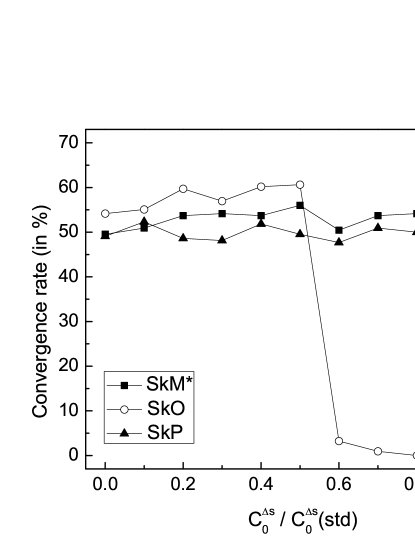
However, other Skyrme parametrizations may be prone to severe and systematic divergences. To illustrate this point, we have performed a set of calculations with three functionals: SkO [Rei99fw] , SkP, and SkM* [Bar82fw] . For each of those, we have used the native variant of the time-odd terms; only is multiplied by a scaling factor ranging between zero (no coupling) and one (standard coupling). A measure of stability of the iterative process is the rate of convergence for a pre-defined set of one-quasiparticle states. A result is deemed converged if the binding energy does not change by more than 2 keV from one iteration to the next for 3 consecutive iterations. We show in Fig. 9 the evolution of this convergence rate as a function of . Our set of configurations consists of 24 different one-quasiproton states in nine odd- Ho isotopes with 88104. Therefore, the sample size used to define the convergence rate is 216.
According to Fig. 9, SkM* and SkP parametrizations are stable with respect to variations of , but the SkO functional exhibits a sharp drop in the convergence rate when , i.e., MeV. Preliminary investigation of the rpa response function [Les09] suggests that instabilities could occur for transferred momenta of the order of 2.2–2.5 fm-1 for this particular value of . These results nicely agree with the original findings of [Les06] and emphasize the need of testing edfs against finite-size instabilities.
V Conclusions
In this work, we carried out the systematic theoretical survey of one-quasiproton states in deformed rare-earth nuclei. Our study is based on the symmetry-unconstrained Skyrme hfb framework that fully takes into account time-odd polarization effects.
We show that the equal filling approximation is equivalent to the full blocking when the time-odd fields are put to zero. In this case, an arbitrary combination of time-reversed orbits can be used to define the blocked orbit, and this can be nicely quantified by introducing the notion of alispin. We emphasize the role of symmetries, and in particular nuclear alignment properties, in the exact treatment of the blocked state.
Our systematic survey indicates that, when native functionals are employed, the contributions from time-odd fields to the energy of the g.s. and low-lying excited states is rather small, around 50 keV on average, with a variation around 100–150 keV. Significant differences are found from one interaction to another, although the effect remains small for the three interactions considered. Correcting the time-odd channel (Landau functionals) increases the contribution of the time-odd channel to the total energy by about 50%. For the functionals in the gauge variant, the time-odd effects are weak and opposite in sign.
By explicit calculations we demonstrated that the choice of the alignment orientation with respect to the quantization axis does impact predicted time-odd polarization energies. The resulting energy shifts are appreciable in the scale of predicted time-odd displacements.
Standard parameterizations of the Skyrme interaction, such as the SIII, SkP, and SLy4, give a qualitative, but not quantitative description of experimental one-quasiproton spectra in the rare-earth region. We find that the triaxial shape polarization effects are generally small in the nuclei considered. Finally, we point to the sensitivity of dft calculations for one-quasiparticle states to finite-size instabilities of the underlying edf. A detailed investigation of this effect is currently under way.
The weak impact of the time-odd fields on spectroscopic properties implies that global studies with symmetry-restricted hfb solvers such as hfbtho could be very useful to extract information related to the isovector properties, shell structure, and shapes. For such a purpose, time-odd fields may be safely neglected.
Acknowledgements.
We are thankful to T. Duguet and T. Lesinski for pointing out finite-size instabilities as a possible explanation for the systematic lack of convergence in odd nuclei with certain functionals. Discussions with S. Fracasso are also acknowledged. This work was supported by the U.S. Department of Energy under Contract Nos. DE-FC02-07ER41457 (UNEDF SciDAC Collaboration), DE-FG02-96ER40963 (University of Tennessee), DE-AC05-00OR22725 with UT-Battelle, LLC (Oak Ridge National Laboratory), and DE-FG0587ER40361 (Joint Institute for Heavy Ion Research); by the Polish Ministry of Science and Higher Education under Contract No. N N 202 328234; and by the Academy of Finland and University of Jyväskylä within the FIDIPRO program. Computational resources were provided by the National Center for Computational Sciences at Oak Ridge National Laboratory.References
- [1] I.Zh. Petkov and M.V. Stoitsov. Nuclear Density Functional Theory. Clarendon Press, Oxford, 1991. Oxford Studies in Physics, volume 14.
- [2] M. Bender, P.-H. Heenen, and P.-G. Reinhard, Rev. Mod. Phys. 75, 121 (2003).
- [3] Extended Density Functionals in Nuclear Structure Physics, ed. by G.A. Lalazissis, P. Ring, and D. Vretenar (Springer Verlag, 2004).
- [4] M.V. Stoitsov, J. Dobaczewski, W. Nazarewicz, and P. Borycki, Int. J. Mass Spectrometry 251, 243 (2006).
- [5] G.F. Bertsch, B. Sabbey, and M. Uusnäkki, Phys. Rev. C 71, 054311 (2005).
- [6] M. Zalewski, J. Dobaczewski, W. Satuła, and T.R. Werner, Phys. Rev. C 77, 024316 (2008).
- [7] M. Kortelainen, J. Dobaczewski, K. Mizuyama, and J. Toivanen, Phys. Rev. C 77, 064307 (2008).
- [8] G.F. Bertsch, D.J. Dean, and W. Nazarewicz, SciDAC Review 6, Winter 2007, p. 42.
- [9] J.W. Negele and D. Vautherin, Phys. Rev. C 5, 1472 (1972).
- [10] S.K. Bogner, R.J. Furnstahl, and L. Platter, Eur. Phys. J. A 39, 219 (2009).
- [11] B.G. Carlsson, J. Dobaczewski, and M. Kortelainen, Phys. Rev. C 78, 044326 (2008).
- [12] T. Lesinski, M. Bender, K. Bennaceur, T. Duguet, and J. Meyer, Phys. Rev. C 76, 014312 (2007).
- [13] W. Satuła, R.A. Wyss and M. Zalewski, Phys. Rev. 78, 011302(R) (2008).
- [14] W. Satuła, M. Zalewski, J. Dobaczewski, P. Olbratowski, M. Rafalski, T.R. Werner and R.A. Wyss, Int. J. Mod. Phys. E 18, 808 (2009).
- [15] J. Margueron, S. Goriely, M. Grasso, G. Coló, and H. Sagawa, J. Phys. G: Nucl. Part. Phys. 36, 125103 (2009).
- [16] S. Goriely, N. Chamel and J. M. Pearson, Phys. Rev. Lett. 102, 152503 (2009).
- [17] Y.M. Engel, D.M. Brink, K. Goeke, S.J. Krieger, and D. Vautherin, Nucl. Phys. A 249, 215 (1975).
- [18] E. Perlińska, S.G. Rohoziński, J. Dobaczewski, and W. Nazarewicz, Phys. Rev. C 69, 014316 (2004).
- [19] U. Post, E. Wüst, and U. Mosel, Nucl. Phys. A 437, 274 (1985).
- [20] B.-Q. Chen, P.-H. Heenen, P. Bonche, M.S. Weiss, and H.Flocard, Phys. Rev. C 46, R1582-6 (1992).
- [21] J. Dobaczewski and J. Dudek, Phys. Rev. C 52, 1827 (1995); C 55, 3177(E) (1997).
- [22] A.V. Afanasjev and P.Ring, Phys. Rev. C 62, 031302(R) (2000).
- [23] M. Bender, J. Dobaczewski, J. Engel, and W. Nazarewicz, Phys. Rev. C 65, 054322 (2002).
- [24] K. Rutz, M. Bender, J.A. Maruhn, P.-G. Reinhard, and W. Greiner, Nucl. Phys. A 634, 67 (1998).
- [25] M. Baranger and M. Vénéroni, Ann. Phys. 114 123, (1978).
- [26] J. Dobaczewski and J. Skalski, Nucl. Phys. A 369, 123 (1981).
- [27] J. A. Maruhn, P.-G. Reinhard, P. D. Stevenson and M. R. Strayer, Phys. Rev. C 74, 027601 (2006).
- [28] N. Hinohara, T. Nakatsukasa, M. Matsuo, and K. Matsuyanagi, Prog. Theor. Phys. (Kyoto) 115, 567 (2006).
- [29] W. Ogle, S. Wahlborn, R. Piepenbring and S. Fredriksson, Rev. Mod. Phys. 43, 424 (1971).
- [30] W. Nazarewicz, M.A. Riley, and J.D. Garrett, Nucl. Phys. A 512, 61 (1990).
- [31] S. Ćwiok and W. Nazarewicz, Nucl. Phys. A 529, 95 (1991).
- [32] S. Ćwiok, S. Hofmann, and W. Nazarewicz, Nucl. Phys. A 573, 356 (1994).
- [33] A. Parkhomenko and A. Sobiczewski, Acta Phys. Pol. 36, 3115 (2005).
- [34] K. Rutz, M. Bender, P.-G. Reinhard, and J. Maruhn, Phys. Lett. B 468, 1 (1999).
- [35] S. Ćwiok, W. Nazarewicz, and P.-H. Heenen, Phys. Rev. Lett. 83, 1108 (1999).
- [36] A.V. Afanasjev, T.L. Khoo, S. Frauendorf, G.A. Lalazissis, and I. Ahmad, Phys. Rev. C 67, 024309 (2003).
- [37] A.V. Afanasjev and H. Abusara, Phys. Rev. C 81, 014309 (2010).
- [38] L. Bonneau, P. Quentin and P. Möller, Phys. Rev. C 76, 024320 (2007).
- [39] J. R. Stone and P.-G. Reinhard, Prog. Part. and Nucl. Phys. 58, 587 (2007).
- [40] A. Bulgac, Preprint FT-194-1980, Central Institute of Physics, Bucharest, 1980; nucl-th/9907088.
- [41] J. Dobaczewski, H. Flocard and J. Treiner, Nucl. Phys. A 422, 103 (1984).
- [42] J. Dobaczewski, W. Nazarewicz, T.R. Werner, J.-F. Berger, C.R. Chinn, and J. Dechargé, Phys. Rev. C 53, 2809 (1996).
- [43] J.P. Blaizot and G. Ripka. Quantum theory of finite systems. MIT Press, 1986.
- [44] P. Ring and P. Schuck. The Nuclear Many-Body Problem. Springer Verlag, Berlin, 1980.
- [45] B. Banerjee, P. Ring, and H.J. Mang, Nucl. Phys. A 221, 564 (1974).
- [46] A. Faessler, M. Płoszajczak, and K.W. Schmid, Prog. Part. Nucl. Phys. 5, 79 (1980).
- [47] G. Bertsch, J. Dobaczewski, W. Nazarewicz and J. Pei, Phys. Rev. A 79, 043602 (2009).
- [48] S. Perez-Martin and L.M. Robledo Phys. Rev. C 78, 014304 (2008).
- [49] P.-H. Heenen, P. Bonche and H. Flocard, Nucl. Phys. A 588, 490 (1995).
- [50] J. Dobaczewski, W. Satuła, B.G. Carlsson, J. Engel, P. Olbratowski, P. Powałowski, M. Sadziak, J. Sarich, N. Schunck, A. Staszczak, M.V. Stoitsov, M. Zalewski, and H. Zduńczuk, Comput. Phys. Commun. 180, 2361 (2009).
- [51] S. Perez-Martin and L.M. Robledo, Phys. Rev. C 76, 064314 (2007).
- [52] P. Olbratowski, J. Dobaczewski, and J. Dudek, Phys. Rev. C 73, 054308 (2006).
- [53] D.A. Varshalovich, A.N. Moskalev and V.K. Khersonskii. Quantum Theory of Angular Momentum. World Scientific, Singapore, 1988.
- [54] P. Olbratowski, J. Dobaczewski, J. Dudek, and W. Płóciennik, Phys. Rev. Lett. 93, 052501 (2004).
- [55] J. Dobaczewski and J. Dudek, Comput. Phys. Commun. 102, 166 (1997); 102, 183 (1997), 131, 164 (2000), J. Dobaczewski and P. Olbratowski, ibid. 158, 158 (2004).
- [56] M. Girod and B. Grammaticos, Phys. Rev. C 27, 2317 (1983).
- [57] M.V. Stoitsov, J. Dobaczewski, W. Nazarewicz, and P. Ring, Comput. Phys. Commun. 167, 43 (2005).
- [58] J. Dobaczewski and P. Olbratowski, Comput. Phys. Commun. 167, 214 (2005).
- [59] M. Stoitsov J. Dobaczewski and W. Nazarewicz. In NUCLEAR PHYSICS, LARGE and SMALL, Microscopic Studies of Collective Phenomena, volume 726 of AIP Conference Proceedings, page 52, New-York, 2004. American Institute of Physics. Ed. by R. Bijker, R.F. Casten, and A. Frank.
- [60] J. Dobaczewski and J. Dudek, Comput. Phys. Commun. 102, 166 (1997); 102, 183 (1997).
- [61] M. Beiner, H. Flocard, N. Van Giai, and P. Quentin, Nucl. Phys. A 238, 29 (1975).
- [62] E. Chabanat, P. Bonche, P. Haensel, J. Meyer, and R. Schaeffer, Nucl. Phys. A 635, 231 (1998).
- [63] J. Dobaczewski, W. Nazarewicz, and M. V. Stoitsov, Eur. Phys. J. A 15, 21 (2002).
- [64] A. Bulgac and Y. Yu, Phys. Rev. Lett. 88, 042504 (2002).
- [65] P.J. Borycki, J. Dobaczewski, W. Nazarewicz, and M.V. Stoitsov, Phys. Rev. C 73, 044319 (2006).
- [66] G. F. Bertsch, C. A. Bertulani, W. Nazarewicz, N. Schunck and M. V. Stoitsov, Phys. Rev. C 79, 034306 (2009).
- [67] T. Lesinski, T. Duguet, K. Bennaceur, and J. Meyer, Eur. Phys. J. A 40, 121 (2009).
- [68] D.D. Johnson, Phys. Rev. B 38, 12807 (1988).
- [69] A. Baran, A. Bulgac, M. McNeil Forbes, G. Hagen, W. Nazarewicz, N. Schunck, and M.V. Stoitsov, Phys. Rev. C 78, 014318 (2008).
- [70] T. Duguet, P. Bonche, P.-H. Heenen, and J. Meyer, Phys. Rev. C 65, 014310 (2001).
- [71] T. Duguet, P. Bonche, P.-H. Heenen, and J. Meyer, Phys. Rev. C 65, 014311 (2001).
- [72] H. Zduńczuk, W. Satuła and R.A. Wyss, Phys. Rev. C 71 , 024305 (2005).
- [73] S. Fracasso, G. Coló, Phys. Rev. C 76, 044307 (2007).
- [74] A. Bohr and B.R. Mottelson. Nuclear Structure, volume II. Benjamin, New-York, 1975.
- [75] Evaluated Nuclear Structure Data File.
- [76] B.S. Nielsen and M.E. Bunker, Nucl. Phys. A 245, 376 (1975).
- [77] Z. Szymański. Fast Nuclear Rotation. Clarendon Press, Oxford, 1983.
- [78] S. Frauendorf, Rev. Mod. Phys. 73, 463 (2001).
- [79] T. Shoji and Y. R. Shimizu, Prog. Theor. Phys. 121, 319 (2009).
- [80] S.W. Ødegård et al., Phys. Rev. Lett. 86, 5866 (2001).
- [81] D.R. Jensen et al., Phys. Rev. Lett. 89, 142503 (2002).
- [82] S. Frauendorf and J. Meng, Nucl. Phys. A 617, 131 (1997).
- [83] B. Qi, S. Q. Zhang, J. Meng, S. Y. Wang and S. Frauendorf, nucl-th/arXiv:0812.4597.
- [84] P. Möller, R. Bengtsson, B. G. Carlsson, P. Olivius and T. Ichikawa, Phys. Rev. Lett. 97, 162502 (2006).
- [85] S. Frauendorf and F.R. May, Phys. Lett. B 125, 245 (1983).
- [86] I. Hamamoto and B. Mottelson, Phys. Lett. B 127, 281 (1983).
- [87] S. Åberg, Nucl. Phys. A 520 (1990).
- [88] M. Matev, A.V. Afanasjev, J. Dobaczewski, G.A. Lalazissis and W. Nazarewicz, Phys. Rev. C 76, 034304 (2007).
- [89] I. Hamamoto and B. Mottelson, Phys. Lett. B 127, 281 (1983).
- [90] J. P. Blaizot, Phys. Lett. B 60, 435 (1976).
- [91] E. Caurier and B. Grammaticos, Phys. Lett. B 92, 236 (1980).
- [92] T. Lesinski, K. Bennaceur, T. Duguet and J. Meyer, Phys. Rev. C 74, 044315 (2006).
- [93] A.L. Fetter and J.D. Walecka. Quantum Theory of Many-Particle Systems. McGraw-Hill, Boston, 1971.
- [94] C. García-Recio, J. Navarro, N. Van Giai and N. N. Salcedo, Ann. of Phys. 214, 293 (1992).
- [95] J. Margueron, J. Navarro, N. Van Giai, Phys. Rev. C 74, 015805 (2006).
- [96] P.-G. Reinhard, D.J. Dean, W. Nazarewicz, J. Dobaczewski, J.A. Maruhn, and M.R. Strayer, Phys. Rev. C 60, 014316 (1999).
- [97] J. Bartel, P. Quentin, M. Brack, C. Guet, and H.B. Håkansson, Nucl. Phys. A 386, 79 (1982).
- [98] T. Lesinski, Private Communication (2009).