Orbital selective local moment formation in iron: first principle route to an effective model

Abstract

We revisit a problem of theoretical description of $\alpha$-iron. By performing LDA+DMFT calculations in the paramagnetic phase we find that Coulomb interaction and, in particular Hund exchange, yields the formation of local moments in $e_{g}$ electron band, which can be traced from imaginary time dependence of the spin-spin correlation function. This behavior is accompanied by non-Fermi-liquid behavior of $e_{g}$ electrons and suggests using local moment variables in the effective model of iron. By investigating orbital-selective contributions to the Curie-Weiss law for Hund exchange $I=0.9$ eV we obtain an effective value of local moment of $e_{g}$ electrons $2p=1.04\mu_{B}$. The effective bosonic model, which allows to describe magnetic properties of iron near the magnetic phase transition, is proposed.

I Introduction

The magnetism and its influence to properties of materials attracts a lot of interest since ancient ages, first records can be traced back to Greek philosopher Thales of Miletus and Indian surgeon Sushruta about 600 BC. In particular, the problem of origin of ferromagnetism of iron attracts a lot of attention, despite long time of its investigations.

The $d$-electrons in iron (as well as in many other transition metals) show both, localized, and itinerant behavior. According to the Rhodes and Wolfarth criterion, iron is classified as a local moment system, since the ratio of the magnetic moment $2p_{\text{CW}}\mu_{B}$ corresponding to the effective spin $p_{\text{CW}}$ extracted from Curie-Weiss law for susceptibility $\chi=g^{2}\mu_{B}^{2}p_{\text{CW}}(p_{\text{CW}}+1)/(3(T-T_{C}))$ ($g\approx 2$ is the $g$-factor, $\mu_{B}$ is the Bohr magneton, $T_{C}$ being the Curie temperature) to the magnetic moment per atom in the ferromagnetic phase, $2p_{\text{CW}}\mu_{B}/\mu_{\text{exp}}=1.05$ is close to unity (see, e.g. Ref. Moriya, ). At the same time, the experimental magnetic moment of iron $\mu_{\exp}=2.2\mu_{B}$ is not an integer number, which indicates presence of some fraction of itinerant electrons.

Itinerant theory of magnetism of transition metals was pioneered by Stoner, and then became a basis of spin-fluctuation theory by Moriya Moriya which was successful to describe weak and nearly ferro- and antiferromagnetic materials. By considering fluctuation corrections to mean field, Moriya theory was able to reproduce nearly Curie-Weiss behavior of magnetic susceptibility and to obtain correct values of transition temperatures of weak or nearly magnetic systems. At the same time, this theory meets serious difficulties when applied to materials with large magnetic moment, such as some transition metals. These materials are expected to be better described in terms of the local moment picture. In practice, to describe $d$-electrons in transition metals in the semi-phenomenological way, the localized-moment (Heisenberg) model is often used. Band structure calculations of magnetic exchange interaction in iron show however its non-Heisenberg character at intermediate and large momenta Licht . Using microscopic consideration Mott Mott proposed a two-band model for transition metals with narrow band of $d$-electrons and wide band of $s$-electrons. The polar $s$-$d$ model, which treats $d$-electrons as localized and $s$-electrons as itinerant was proposed by Shubin and Vonsovskii Shubin .

First attempts to unify the localized and itinerant pictures of magnetism were performed in Refs. Hubbard, ; Moriya, for the single and degenerate band models, respectively. To unify localized and itinerant approaches to magnetism and find an origin of the formation of local moments, it seems however important to consider the orbital-resolved contributions to one- and two-particle properties. In particular, it was suggested by Goodenough Goodenough that the the electrons with $e_{g}$ and $t_{2g}$ symmetry may behave very differently in iron: while the former show localized, the latter may show itinerant behavior. The “95% localized model” of iron was proposed by Stearns Stearns according to which 95% of $d$-electrons are localized, while 5% are itinerant. This idea found its implementation in the “two-band model” Mota , which was considered within the mean-field approach. Later on it was suggested KatsVH ; KatsVH1 that the states at the van Hove singularities may induce localization of some $d$-electron states. However, no microscopic evidences for such localization were obtained so far.

The important source of the local moment formation are strong electronic correlations. In particular, the ferromagnetic state of the one-band strongly-correlated Hubbard model, which was shown to be stable for sufficiently large on-site Coulomb repulsionUhrig ; DMFTFerro , has linear dependence of the inverse susceptibility above transition temperature within the dynamical mean-field theory (DMFT)DMFTFerro . The role of interband Coulomb interaction and Hund exchange in non-degenerate Hubbard model to reduce the critical intraband Coulomb interaction strength was emphasized in Refs. DMFTFerroMultiorb, ; Rio, .

To get insight in the applicability of the abovementioned proposals to mechanism of local moment formation in iron, the combination of first-principleManning ; Callaway ; Abate and model calculations seems necessary. The recently performed LDA+DMFT calculationsKatsPRL allowed to describe quantitatively correct the magnetization and susceptibility of iron as a function of the reduced temperature $T/T_{C};$ in particular they led to almost linear temperature dependence of the inverse static spin susceptibility above the magnetic transition temperature, which is similar to the results of model calculations and can be considered as possible evidence for existence of local moments. The estimated magnetic transition temperature appears however twice large than the experimental value $T_{C}=1043K$. The one-particle properties below the transition temperature were addressed in Refs. MagnDMFT, ; KatsLicht, . To get insight into the mechanism of the formation of local moments and linear dependence of susceptibilities above the Curie temperature it seems however important to study one- and two-particle properties in the symmetric phase.

To this end we reconsider in the present paper ab initio LDA+DMFT calculations, paying special attention to orbital-resolved contributions to one- and two-particle properties. Contrary to previously accepted view that Hund exchange only helps to form ferromagnetic state, we argue that in fact it serves as a main source of formation of local moments in iron, together with the almost absent hybridization between $t_{2g}$ and $e_{g}$ bands. These two factors yield formation of local moments for the $e_{g}$ states, while $t_{2g}$ states remain more itinerant.

II The $d$-electron model and orbital-selective magnetic moments

To discuss the behavior of $d$-electrons in iron let us start from standard multi-band Hubbard Hamiltonian

$$\hat{H}^{d} =\hat{H}_{\text{kin}}+\hat{H}_{\text{int}}^{d}$$ (1)

$$+ \sum_{\mathbf{k}}\sum\limits_{mm^{\prime}\sigma}t_{mm^{\prime}}(\mathbf{k})\hat{c}_{\mathbf{k}m\sigma}^{\dagger}\hat{c}_{\mathbf{k}m^{\prime}\sigma}$$

$$+ \frac{1}{2}\sum_{i}\sum\limits_{\{m\}\sigma\sigma^{\prime}}\langle m,m^{\prime}|V_{ee}|m^{\prime\prime},m^{\prime\prime\prime}\rangle\hat{c}_{im\sigma}^{\dagger}\hat{c}_{im^{\prime}\sigma^{\prime}}^{\dagger}\hat{c}_{im^{\prime\prime}\sigma}\hat{c}_{im^{\prime\prime\prime}\sigma^{\prime}},$$

where the first term represents a kinetic contribution to Hamiltonian and the second one is an interaction part. $c_{\mathbf{k}m\sigma}^{\dagger}(c_{\mathbf{k}m\sigma})$ are creation (annihilation) operators for electron with respective quantum indices $|\mathbf{k}m\sigma\rangle$ and $c_{im\sigma}^{\dagger}$ is a Fourier image in real space. $t_{mm^{\prime}}(\mathbf{k})$ is a dispersion and $\langle m,m^{\prime}|V_{ee}|m^{\prime\prime},m^{\prime\prime\prime}\rangle$ is a Coulomb interaction matrix. For a sake of simplicity we assume that orbital index $m$ runs over the correlated $d$-orbitals only.

Keeping a density-density and spin-flip terms in the interacting part of above Hamiltonian (Eq. 1) and assuming a simple parametrization of the interaction matrix with the intraorbital Coulomb interaction, $U=\langle m,m|V_{ee}|m,m\rangle$, the interorbital Coulomb interaction, $U^{\prime}=\langle m,m^{\prime}|V_{ee}|m,m^{\prime}\rangle$ and Hund’s exchange, $I=\langle m,m^{\prime}|V_{ee}|m^{\prime},m\rangle$ one can rewrite the interaction as

$$H_{\text{int}}^{d} =U\sum\limits_{im}\hat{n}_{im\uparrow}\hat{n}_{im\downarrow}+(U^{\prime}-\frac{I}{2})\sum\limits_{i,m<m^{\prime},\sigma\sigma^{\prime}}\hat{n}_{im\sigma}\hat{n}_{im^{\prime}\sigma^{\prime}}$$ (2)

$$-2I\sum\limits_{i,m<m^{\prime}}\hat{\mathbf{s}}_{im}\hat{\mathbf{s}}_{im^{\prime}},$$

where $m$ runs over all $d$-orbital indices and

$$\hat{n}_{im\sigma} =\hat{c}_{im\sigma}^{\dagger}\hat{c}_{im\sigma},$$

$$\hat{\mathbf{s}}_{im} =\frac{1}{2}\sum\limits_{\sigma\sigma^{\prime}}\hat{c}_{im\sigma}^{\dagger}\boldsymbol{\sigma}_{\sigma\sigma^{\prime}}\hat{c}_{im\sigma^{\prime}}.$$

$\boldsymbol{\sigma}$ are the Pauli matrices.

Generically, the Coulomb interaction yields loss of coherence of corresponding electronic states. It will be shown in Sec. III, that electrons in weakly hybridized $t_{2g}$ and $e_{g}$ orbitals behave very differently with respect to the Coulomb interaction. While the behavior of $t_{2g}$ electrons remains Fermi liquid like, $e_{g}$ electrons form a non-Fermi liquid states that implies formation of local moments. Magnetic properties of the resulting system can be then understood in terms of an effective model, containing spins of local and itinerant electron subshells.

Splitting in Eq. (2) contributions of $e_{g}$ and $t_{2g}$ electrons and neglecting hybridization between them (which will be shown to be small in Sec. III.1), we can rewrite the Hamiltonian (1) as

$$\hat{H}^{d} =\hat{H}^{t_{2g}}+\hat{H}^{e_{g}}-2I\sum\limits_{i,m\in t_{2g}}\hat{\mathbf{S}}_{i}\hat{\mathbf{s}}_{im}$$ (3)

$$+(U^{\prime}-\frac{I}{2})\sum\limits_{i,\sigma,m\in t_{2g}}\hat{N}_{i}\hat{n}_{im\sigma},$$

where $\hat{H}^{t_{2g}}$ and $\hat{H}^{e_{g}}$ are the parts of Hamiltonian (1) acting on the $t_{2g}$ and $e_{g}$ orbitals, respectively, $\hat{\mathbf{S}}_{i}=\sum\nolimits_{m\in e_{g}}\hat{\mathbf{s}}_{im},~{}\hat{N}_{i}=\sum\nolimits_{m\in e_{g}}\hat{n}_{im}$. Note that operators $\hat{\mathbf{S}}_{i}$ do not generically describe fully local moments, but will be shown to have properties close to those of local moments due to Hund exchange interaction. Below after considering the results of band structure calculations, we discuss the effect of interaction in Eq. (3) within DMFT and its implications for the effective model.

III First principle calculations for iron

III.1 Band structure results

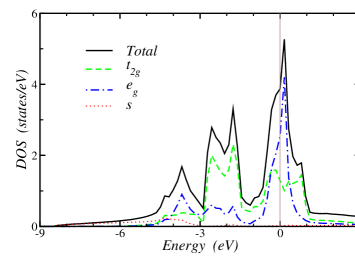
Figure 1: (Color online) Iron density of states obtained within LDA approximation. Total DOS is shown by solid (black) line. Partial $t_{2g}$, $e_{g}$ and $s$ DOSes are shown by (green) dashed, (blue) dot-dashed and (red) dot lines, respectively.

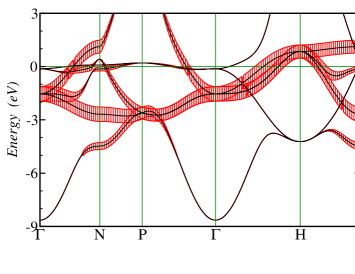
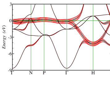
Figure 2: (Color online) The band structure of Fe along high symmetry lines in the Brillouin zone obtained within LDA approximation. The contribution of $t_{2g}$ (left panel) and $e_{g}$ (right panel) states is shown with fat (red) lines.

Iron crystallizes in body centered cubic structure below 1183 K and has the lattice parameter $a=2.8664$ Å at room temperature str . Band structure calculations have been carried out in LDA approximation LDA within TB-LMTO-ASA framework Andersen84 . The von Barth-Hedin local exchange correlation potential was used vonbarth . Primitive reciprocal translation vectors were discretized into 12 points along each direction which leads to 72 $\mathbf{k}$-points in irreducible part of the Brillouin zone.

Total and partial densities of states are presented in Fig. 1. The contribution of a wide $s$-band is shown by (red) dots and spreads from -8.5 eV to energies well above the Fermi level (at zero energy); $t_{2g}$ and $e_{g}$ states ((green) dashed and (blue) dot-dashed) span energy region from -5 eV to 1 eV approximately. In spite of almost equal bandwidths of $t_{2g}$ and $e_{g}$ states they are qualitatively different. Former states are distributed more uniformly over the energy range while the later one have a large peak located at the Fermi energy.

The contributions of $t_{2g}$ and $e_{g}$ orbitals to the band structure of iron are presented in Fig. 2 (left and right panels, respectively). The states contributing to the van Hove singularity near the Fermi energy are of mostly $e_{g}$ symmetry. As it was argued in Refs. KatsVH1, and VHS, , despite the three-dimensional character of the band structure, the lines of van Hove singularities, which due to symmetry reasons can easily occur along the $\Gamma-N$ direction, produce a peak in the density of states. In fact, this singularity is actually a part of the flat band going along $\Gamma-N-P-\Gamma$ directions. On the other hand, $t_{2g}$ bands do not have a flatness close to the Fermi level. These peculiarities of the band structure and absence of direct hybridization between $t_{2g}$ and $e_{g}$ states suggest that the $t_{2g}$ and $e_{g}$ electrons may behave very differently when turning on on-site Coulomb interaction.

III.2 DMFT calculations

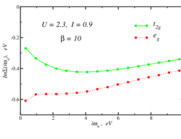
Figure 3: (Color online) The imaginary part of self-energy for $t_{2g}$ (green) solid line and $e_{g}$ states (red) dotted line plotted on the Matsubara (imaginary) energy grid.

In order to take into account correlation effects in 3$d$ shell of $\alpha$-iron the LDA+DMFT method was applied (for detailed description of the computation scheme see Ref. Anisimov05, ). We use the Hamiltonian of Hubbard type as in Eq. (1) with the kinetic term containing all $s-p-d$ states and the interaction part with density-density contributions for $d$-electrons only

$$\hat{H}_{\text{int}} =\frac{1}{2}\sum\limits_{imm^{\prime}\sigma}\Bigl{\{}U_{mm^{\prime}}\hat{n}_{im\sigma}\hat{n}_{im^{\prime}\bar{\sigma}}$$ (4)

$$+(U_{mm^{\prime}}-J_{mm^{\prime}})\hat{n}_{im\sigma}\hat{n}_{im^{\prime}\sigma}\Bigr{\}},$$

where $U_{mm^{\prime}}\equiv\langle m,m^{\prime}|V_{ee}|m,m^{\prime}\rangle$ and $J_{mm^{\prime}}\equiv\langle m,m^{\prime}|V_{ee}|m^{\prime},m\rangle$. Regarding interaction between $d$-electrons, the model (4) serves as a simplified version of the model (1), since it does not contain transverse components of the Hund exchange and pair-hopping term.

The Coulomb interaction parameter value $U$=2.3 eV and the Hund’s parameter $I$=0.9 eV used in our work are the same as in earlier LDA+DMFT calculations by Lichtenstein et al KatsPRL . To treat a problem of formation of local moments we consider paramagnetic phase. The effective impurity model for DMFT was solved by QMC method with the Hirsh-Fye algorithm HF86 . Calculations were performed for the value of inverse temperature $\beta$=10 eV^-1 which is close to the $\alpha\rightarrow\gamma$ transition temperature. Inverse temperature interval $0<\tau<\beta$ was divided in 100 slices. 4 million QMC sweeps were used in self-consistency loop within LDA+DMFT scheme and up to 12 million of QMC sweeps were used to calculate spectral functions.

In Fig. 3 the imaginary part of self-energies are shown for the imaginary frequency axis. One can clearly see that the behavior of $\Im\Sigma(i\omega_{n})$ at low energies is qualitatively different for different orbitals. While $\Im\Sigma(i\omega_{n})$ for $t_{2g}$ states has a Fermi-liquid-like behavior with the quasiparticle weight $Z$=0.86, zero energy outset $\Re\Sigma(0)\simeq 1.1$ eV, and damping $\Im\Sigma(0)=-0.22$ eV, the $\Im\Sigma(i\omega_{n})$ for $e_{g}$ orbitals has a divergent-like shape indicating a loss of coherence regime. As it will be shown in the Section III.3, the latter states form local magnetic moments. This fact affords a ground for separation of the iron $d$-states onto two subsystems: more localized $e_{g}$-states and itinerant $t_{2g}$-states. Contrary to the picture proposed in Ref. KatsVH, , we find not only localization of electrons, contributing to the van Hove singularity states, but most part of $e_{g}$ electrons is expected to form local moments. The features observed for $e_{g}$ states are similar to those observed near Mott metal insulator transition Bulla (see also the results on the real axis below in Fig. 4), although in our case non-Fermi liquid behavior touches only part of the states and the metal-insulator transition does not happen. We have verified that the obtained results depend very weakly on $U$ in the range $U=2\div 6$ eV, while switching off (or reducing) $I$ immediately suppresses non-Fermi-liquid contributions. Therefore, Hund exchange serves as a major source of local moment formation of $e_{g}$ states.

Fig. 4 shows the resulting behavior of real and imaginary parts of the self-energy of different orbitals on the real axis. To make an analytic continuation of the complex function we used Pade approximation method pade with energy mesh containing both, low- and high energy frequencies. To satisfy high-frequency behaviour the equality of the first three moments of function calculated on the real and imaginary axis was fullfilled. Altogether this procedure garantees an accurate description of the function close to Fermi level and at high-energy. In compliance with the observations from imaginary axis, $\Re\Sigma(\omega)$ has slightly negative slope for $t_{2g}$ states, accompanied by the maximum of $\Im\Sigma(\omega)$ at the Fermi level, while for $e_{g}$ states $\Re\Sigma(\omega)$ has positive slope and $\Im\Sigma(\omega)$ is minimal at the Fermi level. The characteristic energy scale for the observed non-Fermi liquid behavior is of the order of 1 eV, i.e. the Hund exchange parameter, which is too small to produce Hubbard subbands, see straight lines in Fig. 4. Seemingly, the observed features represent stronger breakdown of the Fermi liquid behavior, than $\Im\Sigma\varpropto T^{1+\alpha}$ obtained earlier in the three-band Hubbard model werner .

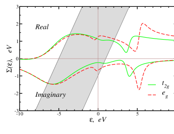
Figure 4: (Color online) The self-energy for $t_{2g}$ (green) solid line and $e_{g}$ states (red) dashed line plotted on the real energy axis. Straight lines $\Sigma=\omega+E_{\text{min,max}}$, which bound shaded area, correspond to the bottom ($E_{\text{min}}$) and top ($E_{\text{max}}$) of the band.

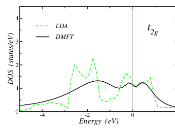
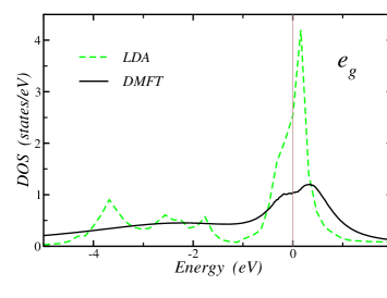
Figure 5: (Color online) The iron $t_{2g}$ (left panel) and $e_{g}$ (right panel) partial density of states obtained within LDA+DMFT method (black solid lines) compared with LDA DOS (green dashed lines).

Partial densities of states obtained in paramagnetic LDA+DMFT calculation for $t_{2g}$ and $e_{g}$ electrons are presented in Fig. 5. The LDA+DMFT densities of states are slightly narrower than the LDA counterparts implying weak correlation effects. One can observe that peak of $e_{g}$ density of states observed in LDA approach is suppressed in LDA+DMFT calculation and split into two peaks at $-0.3$ and 0.5 eV due to non-Fermi-liquid behavior of these states. As discussed above, this splitting should be distinguished from the Hubbard subbands formation near Mott metal-insulator transition, e.g. due to much smaller energy scale, which is of the order of Hund exchange interaction. The shape of $t_{2g}$ density of states in LDA+DMFT approach resembles the LDA result with smearing of the peaky structures of density of states by correlations.

III.3 DMFT spin susceptibility

To discuss the effect of the non-quasiparticle states of $e_{g}$ electrons on magnetic properties we consider imaginary time dependence of the impurity spin susceptibilities

$$\chi_{e_{g}}(\tau) = \sum\limits_{mm^{\prime}\in e_{g}}\langle T[\hat{s}_{im}^{z}(\tau)\hat{s}_{im^{\prime}}^{z}(0)]\rangle=\langle T[\hat{S}_{i}^{z}(\tau)\hat{S}_{i}^{z}(0)]\rangle$$

$$\chi_{t_{2g}}(\tau) = \sum\limits_{mm^{\prime}\in t_{2_{g}}}\langle T[\hat{s}_{im}^{z}(\tau)\hat{s}_{im^{\prime}}^{z}(0)]\rangle$$

obtained within DMFT. The results for the time dependence of $\chi_{e_{g}}(\tau)$, $\chi_{t_{2g}}(\tau),$ and total impurity susceptibility $\chi(\tau)$ for $U=2.3$ eV and $I=0.9$ eV are shown on the insets of Fig. 6. One can see that the dependence $\chi_{e_{g}}(\tau)$ on imaginary time is more flat than $\chi_{t_{2g}}(\tau)$. This fact reflects the formation of local moments for $e_{g}$ electrons, which would correspond to fully time-independent $\chi_{e_{g}}(\tau)$. Switching off $I$ suppresses susceptibility at the flat parts, destroying therefore local moments.

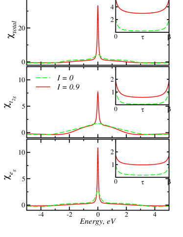
Figure 6: (Color online) Impurity spin susceptibility for the value of Coulomb interaction, $U$ = 2.3 eV, inverse temperature, $\beta$=10 eV^-1 and Hund coupling, $I$=0 (green dashed) and 0.9 eV (red solid) plotted on the real axis. Total impurity spin susceptibility and $t_{2g}$ and $e_{g}$ contributions are shown from top to bottom. The insets show the corresponding imaginary time data.

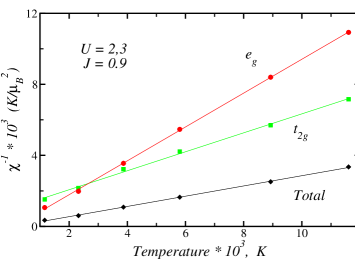
Figure 7: (Color online) Temperature dependence of inverse of the local spin susceptibility. Total spin susceptibility and orbital resolved contributions are presented by (black) diamonds, (green) squares ($t_{2g}$) and (red) circles ($e_{g}$), respectively. Lines are least-square fitting to the original data.

The observed behavior as a function of imaginary time is also reflected as a function of real frequency (Fig. 6). One can see that flat part of the imaginary-time dependence of the susceptibilities yields peak in the real frequency dependence, which is mostly pronounced for $e_{g}$ states. The peak contributions are similar to the frequency dependence of susceptibility of an isolated spin $p$ (note neglection of spatial correlations in DMFT), $\chi(i\omega_{n})=g^{2}\mu_{B}^{2}p(p+1)/(3T)\delta_{n,0}$ and show presence of local moment for $e_{g}$ states. For $t_{2g}$ states we observe mixed behavior with peak contribution transferred from $e_{g}$ states via Hund exchange (see Sect. IV) and incoherent background, originating from $t_{2g}$ itinerant states. This peaky contribution to susceptibilities disappear with switching off $I$, which shows once more that Hund exchange is the major source of the local moment formation.

One of the most transparent characteristic features of the local moment formation is the fulfillment of the Curie-Weiss law for the temperature dependence of the susceptibility. In particular, in the limit of local moments the magnetic moment $\mu_{\text{CW}}$ extracted from Curie-Weiss law is expected to be approximately equal to the magnetic moment in the symmetry-broken phase. The obtained temperature dependence of the local (impurity) susceptibilities is shown in Fig. 7 (the temperature dependence of lattice susceptibilities will be presented elsewhere). One can see that the inverse susceptibility of $e_{g}$ states obeys Curie law with $p_{\text{CW}}(e_{g})=0.52$. The inverse susceptibility of $t_{2g}$ states also shows approximately linear temperature dependence with $p_{\text{CW}}(t_{2g})\simeq 0.7$. The Curie law for the total susceptibility yields $p_{\text{CW}}=1.16$ (the corresponding Curie constant $\mu_{eff}^{2}\equiv g^{2}\mu_{B}^{2}p_{\text{CW}}(p_{\text{CW}}+1)=10\mu_{B}^{2}$) is in good agreement with experimental data and earlier calculations of the lattice susceptibility in the paramagnetic phase KatsPRL . Note close proximity of obtained value $p_{\text{CW}}(e_{g})$ to 1/2.

IV Effective model

The formation of local moments by $e_{g}$ electrons makes the model (3) reminiscent of the multi-band generalization of $s$-$d$ exchange model, supplemented by Coulomb interaction in $t_{2g}$ bands. The $s$-$d$ model was first suggested by Shubin and Vonsovskii to describe magnetism of rare-earth elements and some transition-metal compounds Shubin . Differently to its original formulation, both itinerant and localized states in the model (3) correspond to $d$-electrons, with the $t_{2g}$ and $e_{g}$ orbital symmetry, respectively, and Coulomb interaction in $t_{2g}$ band is present.

Similarly to the diagram technique for the $s$-$d$ model Izyumov , the contribution of the ‘wide band’ $t_{2g}$ electrons can be treat perturbatively. Moreover, we can integrate out electronic degrees of freedom for $t_{2g}$ band and pass to purely bosonic model in a spirit of Moriya theory. Specifically, we introduce new variables $\mathbf{t}_{q}^{m}$ for spins of $t_{2g}$ electrons by decoupling interaction terms in $H_{t_{2g}}$ via Hubbard-Stratonovich transformation and summing contributions from different spin directions (the double counted terms are supposed to be subtructed). We treat only magnetic terms of the interaction, since we are interested in magnetic properties. The Lagrangian, which is obtained by Hubbard-Stratonovich transformation after expansion in the Coulomb interaction between $t_{2g}$ states and Hund exchange can be represented in the form

$$L = L_{e_{g}}+\sum\limits_{q,mm^{\prime}}[R_{mm^{\prime}}^{-1}\mathbf{t}_{q}^{m}\mathbf{t}_{-q}^{m^{\prime}}-\Pi_{q}^{mm^{\prime}}(\mathbf{t}_{q}^{m}+2I\mathbf{S}_{q}\mathbf{)(t}_{-q}^{m^{\prime}}+2I\mathbf{S}_{-q})]$$ (5)

$$+\sum\limits_{q_{i},m_{i}}\Lambda_{q_{1}q_{2}q_{3},abcd}^{mm^{\prime}m^{\prime\prime}m^{\prime\prime\prime}}(\mathbf{t}_{q_{1}}^{m}+2I\mathbf{S}_{q_{1}})_{a}(\mathbf{t}_{q_{2}}^{m^{\prime}}+2I\mathbf{S}_{q_{2}})_{b}(\mathbf{t}_{q_{3}}^{m^{\prime\prime}}+2I\mathbf{S}_{q_{3}})_{c}$$

$$\times(\mathbf{t}_{-q_{1}-q_{2}-q_{3}}^{m^{\prime\prime\prime}}+2I\mathbf{S}_{-q_{1}-q_{2}-q_{3}})_{d}$$

where $R_{mm^{\prime}}=U\delta_{mm^{\prime}}+J(1-\delta_{mm^{\prime}}),$ the sums over band indices are taken over $t_{2g}$ states only, $a,b,c,d=x,y,$ or $z,$,

$$\Pi_{q}^{mm^{\prime}} = -\sum\limits_{k}G_{k}^{mm^{\prime}}G_{k+q}^{m^{\prime}m},$$

$$\Lambda_{q_{1}q_{2}q_{3},abcd}^{mm^{\prime}m^{\prime\prime}m^{\prime\prime\prime}} = \frac{1}{16}\text{Tr}(\sigma^{a}\sigma^{b}\sigma^{c}\sigma^{d})\sum\limits_{k}G_{k}^{mm^{\prime}}G_{k+q_{1}}^{m^{\prime}m^{\prime\prime}}G_{k+q_{1}+q_{2}}^{m^{\prime\prime}m^{\prime\prime\prime}}G_{k+q_{1}+q_{2}+q_{3}}^{m^{\prime\prime\prime}m}$$ (6)

$G_{k}^{mm^{\prime}}$ is the matrix of the (interacting) $t_{2g}$ electron Green functions, and we use the $4$-vector notations $q=(i\omega,\mathbf{q})$ etc. Due to non-quasiparticle nature of $e_{g}$ electrons, the interaction acting on $e_{g}$ electrons and mixed $e_{g}$-$t_{2g}$ terms in the interaction need not be decoupled; the former supposed to be accounted within a non-perturbative approach, e.g. DMFT, while the latter are treated perturbatively. In dynamical mean-field theory quantities $\Pi_{q}^{mm^{\prime}}$ and $\Lambda_{q_{1}q_{2}q_{3},abcd}^{mm^{\prime}m^{\prime\prime}m^{\prime\prime\prime}}$ for generic momenta are the functions of frequencies only.

The Lagrangian (5) can be viewed as the generalization of the standard $\phi^{4}$ model of the magnetic transition of itinerant electrons Moriya ; Hertz to the case of presence of nearly local moments. For the susceptibilities of $t_{2g}$ and $e_{g}$ electrons, and mixed $t_{2g}$-$e_{g}$ susceptibility $\upsilon_{q}$ we obtain up to second order in $I$

$$\left(\begin{array}[]{cc}(R\chi_{q,t_{2g}}+I)R&\upsilon_{q}R\\ \upsilon_{q}R&\chi_{q,e_{g}}\end{array}\right)\begin{array}[]{c}=\end{array}$$ (10)

$$= \left(\begin{array}[]{cc}(\chi_{q,t_{2g}}^{0})^{-1}+\Lambda\ast\chi_{t_{2g}}^{0}+4I^{2}\Lambda\ast\chi_{e_{g}}^{0}&-2I\Pi_{q}\\ -2I\Pi_{q}&(\chi_{q,e_{g}}^{0})^{-1}-4I^{2}\Pi_{q}+4I^{2}\Gamma^{(4)}\ast\chi_{t_{2g}}^{0}\end{array}\right)^{-1}$$ (13)

where $\chi_{q,t_{2g}}^{0}=(R_{mm^{\prime}}^{-1}-\Pi_{q}^{mm^{\prime}})^{-1}$ is the RPA spin susceptibility of $t_{2g}$ band, $\chi_{q,e_{g}}^{0}=\langle\mathbf{S}_{q}\mathbf{S}_{-q}\mathbf{\rangle}_{e_{g}}/3$ is the bare susceptibility of $e_{g}$ band, evaluated with $L_{e_{g}}$,

$$\Gamma_{q_{1}q_{2}q_{3}}^{(4),abcd} = \langle S_{q_{1}}^{a}S_{q_{2}}^{b}S_{q_{3}}^{c}S_{-q_{1}-q_{2}-q_{3}}^{d}\mathbf{\rangle}_{e_{g}}\mathbf{-}\chi_{q_{1},e_{g}}^{0}\chi_{q_{3},e_{g}}^{0}\delta_{q_{1},-q_{2}}$$ (14)

$$-\chi_{q_{1},e_{g}}^{0}\chi_{q_{2},e_{g}}^{0}(\delta_{q_{2},-q_{3}}+\delta_{q_{1},-q_{3}})$$

is the 4-spin Green function, $\ast$ denote the convolution of momenta-, frequency, and band indices. Again, within DMFT the quantities $\chi_{e_{g},q}^{0}$ and $\Gamma_{q_{1}q_{2}q_{3}}^{(4),abcd}$ are only frequency dependent.

The form of the susceptibilities (13) allows in particular to understand the mechanism of fulfillment the Curie law for local susceptibilities of both, $t_{2g}$ and $e_{g}$ electrons and their frequency dependence. While $e_{g}$ electrons form local moments, $\chi_{e_{g}}^{0}$ becomes almost static and shows inverse linear temperature dependence, similar to that obtained in the Heisenberg model. The contribution $4I^{2}\Pi_{q}$ corresponds to RKKY interaction and expected to be weakly temperature dependent. Presumably small contribution $4I^{2}\Gamma^{(4)}\ast\chi_{t_{2g}}^{0}$ can also add some linear in temperature dynamic contribution to the inverse susceptibility of $e_{g}$ electrons. Note that within DMFT this contribution is accounted only in average with respect to momenta, and does not allow to resolve peculiar physics, which arises due to contribution of small momenta (forward scattering). The convolutions $\Lambda\ast\chi_{t_{2g}}$ and $4I^{2}\Lambda\ast\chi_{e_{g}}$ determine the contributions to the susceptibility of $t_{2g}$ electrons from interaction within $t_{2g}$ band and between $t_{2g}$ and $e_{g}$ bands, respectively, and become also linear functions of temperature similarly to the Moriya theory (where they correspond to the so called $\lambda$-correction). These contributions are however incoherent due to complicated frequency dependence of $\Lambda.$ Finally, the terms $I\Pi_{q}$ mix these two (coherent and incoherent) contributions to the susceptibilities due to interorbital Hund exchange and Coulomb interaction in $t_{2g}$ band.

Therefore, the model (5) allows to understand main features of frequency- and temperature dependence of susceptibilities, observed in the DMFT solution. The derivation of the bosonic model and susceptibilities (13) can further serve as a basis for obtaining non-local corrections to the results of dynamic mean-field theory, e.g. in a spirit of dynamic vertex approximation DGA ; DGA1 .

V Conclusion

We have discussed the origin of the formation of local moments in iron, which is due to the localization of $e_{g}$ electrons. In particular, we observe non-Fermi liquid behavior in $e_{g}$, but not $t_{2g}$ band. This mechanism is very similar to the concept of orbital selective Mott transition, which was earlier introduced in Ref. Anisimov, for Ca_2-xSr_xRuO₄. Although a possibility of a separate Mott transition in narrow bands (in the presence of hybridization with a wide band) was questioned by Liebsch Liebsch , the recent high-precission QMC studies of the two band model have confirmed this possibility Dongen . In our case, obtained non-Fermi liquid behavior of $e_{g}$ electrons yields peak in the frequency dependence of spin-spin correlation function and linear temperature dependence of the magnetic susceptibility of $e_{g}$ electrons with $p_{\text{CW}}=0.52,$ both being characteristic features of local moments, formed in $e_{g}$ band.

The formulated spin-fluctuation approach allows to describe thermodynamic properties in the spin symmetric phase. To describe symmetry broken phase, as well as proximity to the magnetic transition temperature, nonlocal (in particular long-range) correlations beyond DMFT are expected to become important. These correlations are also likely to reduce the DMFT transition temperature closer to its experimental value. Although the systematic treatment of the non-local long-range correlations in the strongly-correlated systems is applied currently mainly to the one-band models DGA ; DGA1 ; Cellular ; Slezak , it was shown recently that even for the three-dimensional systems nonlocal corrections substantially reduce the magnetic transition temperature from its DMFT value DGA1 . Future investigations of nonlocal corrections in multi-band models, together with evaluation of thermodynamic properties, have to be performed.

The presented approach can be also helpful to analyse the electron structure of $\gamma$-iron and mechanism of the structural $\alpha-\gamma$ transformation of iron gammaFe . Existing approaches to this problem often start from the Heisenberg model, where the short-range magnetic order in $\gamma$ phase was suggested as the origin of the $\alpha-\gamma$ transformation trans . This picture may need reinvestigation from the itinerant point of view. The presented approach can be useful also for other substances, containing both, local moments and itinerant electrons.

VI Acknowledgement

The authors thank Jan Kuneš for providing his DMFT(QMC) computer code used in our calculations. Support by the Russian Foundation for Basic Research under Grants No. RFFI-07-02-00041 and RFFI-07-02-01264-a, Civil Research and Development Foundation together with the Russian Ministry of Science and Education through program Y4-P-05-15, Federal Agency for Science and Innovations under Grant No. 02.740.11.0217, the Russian president grant for young scientists MK-1184.2007.2 and Dynasty Foundation, the fund of the President of the Russian Federation for the support for scientific schools NSH 1941.2008.2, the Program of Presidium of Russian Academy of Science No. 7 “Quantum microphysics of condensed matter”, and grant 62-08-01 (by “MMK”, “Ausferr”, and “Intels”) is gratefully acknowledged.

References

- (1) T. Moriya, Spin Fluctuations in Itinerant Electron Magnetism (Springer-Verlag, Berlin, 1985).
- (2) V. A. Gubanov, A. I. Lichtenstein, and A. V. Postnikov, Magnetism and Electronic Structure of Crystals, Springer Verlag (Berlin, Heidelberg, New York), 1992.
- (3) N. F. Mott, Proc. Roy. Soc. 47, 571 (1935)
- (4) S. P. Shubin and S. V. Vonsovski, Proc. Roy. Soc. A145, 159 (1934); S.V. Vonsovski, Magnetism (Wiley, New York, 1974).
- (5) J. Hubbard, Phys. Rev. B 19, 2626 (1979); Phys. Rev. B 20, 4584 (1979).
- (6) J. B. Goodenough, Phys. Rev. 120, 67 (1960)
- (7) M. B. Stearns, Phys. Rev. B 8, 4383 (1973)
- (8) R. Mota and M. D. Coutinho-Filho, Phys. Rev. B 33, 7724 (1986)
- (9) V. Yu. Irkhin, M. I. Katsnelson, A. V. Trefilov, J. Phys.: Cond. Matt. 5, 8763 (1993)
- (10) S. V. Vonsovskii, M. I. Katsnelson, and A. V. Trefilov, Fiz. Metallov. Metalloved. 76, issue 3, p. 4 (1993); 76, issue 4, p. 3 (1993).
- (11) T. Hanisch, Götz S. Uhrig, and E. Müller-Hartmann, Phys. Rev. B 56, 13960 (1997).
- (12) M. Ulmke, Eur. Phys. J. B 1, 301 (1998); T. Obermeier, T. Pruschke, J. Keller, Phys. Rev. B 56, R8479 (1997); J. Wahle, N. Blümer, J. Schlipf, K. Held, D. Vollhardt, Phys. Rev. B 58, 12749 (1998);
- (13) K. Held, D. Vollhardt, Eur. Phys. J. B 5, 473 (1998); D. Vollhardt, N. Blümer, K. Held, M. Kollar, J. Schlipf, M. Ulmke, J. Wahle, Advances in Solid State Physics 38, p. 383 (Vieweg, Wiesbaden, 1999); D. Vollhardt, N. Blümer, K. Held, M. Kollar, Lecture Notes in Physics 580, 191 (Springer, 2001).
- (14) S. Sakai, R. Arita, H. Aoki, Phys. Rev. Lett. 99, 216402 (2007).
- (15) M. F. Manning, Phys. Rev. 63, 190 (1942)
- (16) J. Callaway, Phys. Rev. 99, 500 (1955).
- (17) E. Abate and M. Asdente, Phys. Rev. 140, A1303 (1965).
- (18) A. I. Lichtenstein, M. I. Katsnelson, and G. Kotliar Phys. Rev. Lett. 87, 067205 (2001).
- (19) M. I. Katsnelson and A. I. Lichtenstein, J. Phys. C.: Cond. Matt. 11, 1037 (1999); A. Grechnev, I. Di Marco, M. I. Katsnelson, A. I. Lichtenstein, J. Wills, and O. Eriksson, Phys. Rev. B 76, 035107 (2007).
- (20) M. I. Katsnelson, A. I. Lichtenstein, Phys. Rev. B 61, 8906 (2000); J. Phys.: Cond. Matt. 16, 7439 (2004)
- (21) “Constitution of binary alloys” ed. M. Hansen, New York (1958).
- (22) R. O. Jones and O. Gunnarsson, Rev. Mod. Phys. 61, 689 (1989).
- (23) O.K. Andersen et al., Phys. Rev. Lett. 53, 2571 (1984).
- (24) U von Barth and L Hedin, Journal of Physics C: Solid State Physics, 5, 1629 (1972).
- (25) R. Maglic, Phys. Rev. Lett. 31, 546 (1973).
- (26) V.I. Anisimov et al., Phys. Rev. B 71, 125119 (2005).
- (27) J. E. Hirsch and R. M. Fye, Phys. Rev. Lett. 56, 2521 (1986).
- (28) R. Bulla, T. A. Costi, and D. Vollhardt, Phys. Rev. B 64, 045103 (2001).
- (29) H. J. Vidberg and J. W. Serene, J. Low Temp. Phys. 29, 179 (1977).
- (30) P. Werner, E. Gull, M. Troyer, and A. J. Millis, Phys. Rev. Lett. 101, 166405 (2008).
- (31) Yu. A. Izyumov, F. A. Kassan-Ogly, and Yu. N. Skryabin, Field Methods in the Theory of Ferromagnetism (Nauka, Moscow, 1974) (in russian); Yu. A. Izyumov and Yu. N. Skryabin, Statistical Mechanics of Magnetically Ordered Substances (Consultants Bureau, New York, 1988).
- (32) J. A. Hertz, Phys. Rev. B 14, 3 (1976).
- (33) V. I. Anisimov, I. A. Nekrasov, D. E. Kondakov, T. M. Rice, and M. Sigrist, Europhys. J. B 25, 191 (2002).
- (34) A. Liebsch, Europhys. Lett. 63, 97 (2003); Phys. Rev. Lett. 91, 226401 (2003); Phys. Rev. B 70, 165103 (2004).
- (35) C. Knecht, N. Blümer, and P.G.J. van Dongen, Phys. Rev. B 72, 081103(R) (2005).
- (36) A. Toschi, A. A. Katanin, K. Held, Phys. Rev. B 75, 045118 (2007), K. Held, A. A. Katanin, A. Toschi, Prog. Theor. Phys. Suppl. 176, 117 (2008).
- (37) A. A. Katanin, A. Toschi, K. Held, Phys. Rev. B 80, 075104 (2009).
- (38) A. N. Rubtsov, M. I. Katsnelson, and A. I. Lichtenstein, Phys. Rev. B 77, 033101 (2008); S. Brener, H. Hafermann, A. N. Rubtsov, M. I. Katsnelson, A. I. Lichtenstein, Phys. Rev. B 77, 195105 (2008); A. N. Rubtsov, M. I. Katsnelson, A. I. Lichtenstein, A. Georges, Phys. Rev. B 79, 045133 (2009).
- (39) C. Slezak, M. Jarrell, Th. Maier, J. Deisz, arXiv:cond-mat/0603421 (unpublished).
- (40) see, e.g. O. N. Mryasov, V. A. Gubanov, and A. I. Liechtenstein, Phys. Rev. B 45, 12330 (1992); H. C. Herper, E. Hoffmann, and P. Entel, Phys. Rev. B 60, 3839 (1999); S. V. Okatov, A. R. Kuznetsov, Yu. N. Gornostyrev, V. N. Urtsev, and M. I. Katsnelson, Phys. Rev. B 79, 094111 (2009).
- (41) A. N. Ignatenko, A.A. Katanin, and V.Yu.Irkhin, JETP Letters 87, 615 (2008)