Population Synthesis of Binary
Carbon-enhanced Metal-poor Stars

The carbon-enhanced metal-poor (CEMP) stars constitute approximately one fifth of the metal-poor ($[\mathrm{Fe}/\mathrm{H}]\lesssim-2$) population but their origin is not well understood. The most widely accepted formation scenario, at least for the majority of CEMP stars which are also enriched in $s$-process elements, invokes mass-transfer of carbon-rich material from a thermally-pulsing asymptotic giant branch (TPAGB) primary star to a less massive main-sequence companion which is seen today. Recent studies explore the possibility that an initial mass function biased toward intermediate-mass stars is required to reproduce the observed CEMP fraction in stars with metallicity $[\mathrm{Fe}/\mathrm{H}]<-2.5$. These models also implicitly predict a large number of nitrogen-enhanced metal-poor (NEMP) stars which is not seen. In this paper we investigate whether the observed CEMP and NEMP to extremely metal-poor (EMP) ratios can be explained without invoking a change in the initial mass function. We construct binary-star populations in an attempt to reproduce the observed number and chemical abundance patterns of CEMP stars at a metallicity $[\mathrm{Fe}/\mathrm{H}]\sim-2.3$. Our binary-population models include synthetic nucleosynthesis in TPAGB stars and account for mass transfer and other forms of binary interaction. This approach allows us to explore uncertainties in the CEMP-star formation scenario by parameterization of uncertain input physics. In particular, we consider the uncertainty in the physics of third dredge up in the TPAGB primary, binary mass transfer and mixing in the secondary star. We confirm earlier findings that with current detailed TPAGB models, in which third dredge up is limited to stars more massive than about $1.25\mathrm{\,M_{\odot}}$, the large observed CEMP fraction cannot be accounted for. We find that efficient third dredge up in low-mass (less than $1.25\mathrm{\,M_{\odot}}$), low-metallicity stars may offer at least a partial explanation to the large observed CEMP fraction while remaining consistent with the small observed NEMP fraction.

1 Introduction

One of the most interesting problems in modern stellar astronomy is to explain the existence of a population of carbon-enhanced metal-poor (CEMP) stars in the Galactic halo. The HK (Beers et al., 1992) and Hamburg/ESO (Christlieb et al., 2001) surveys find a large number of CEMP stars among the metal-poor (EMP, $[\mathrm{Fe}/\mathrm{H}]\lesssim-2$) population, at a fraction around 20% (e.g. $9\pm 2\%$ Frebel et al., 2006; $21\pm 2\%$ Lucatello et al., 2006; up to $30\%$ from the SAGA database of Suda et al., 2008 – see below for details).

The CEMP stars are subdivided into four groups depending on the presence or absence of the heavy elements barium and europium (see e.g. Beers & Christlieb, 2005). The most populous group consists of the $s$-process rich CEMP stars, the so-called CEMP-$s$ stars (e.g. Aoki et al., 2007) which display barium enhancements of $[\mathrm{Ba}/\mathrm{Fe}]>+0.5$. These account for about 80 per cent of all CEMP stars. There are also CEMP stars with $r$-process enhancements (the CEMP-$r$ class) and some with both $r$- and $s$-process enhancements (CEMP-$r$+$s$, e.g. Jonsell et al., 2006). Finally, there is a class of CEMP stars which show no enhancement of neutron-capture elements. These are called the CEMP-no stars (Aoki et al., 2002). A detailed review of the various CEMP subgroups can be found in Masseron et al. (2009).

A quantitative understanding of the origin of CEMP stars touches on many branches of stellar astronomy. The most likely formation mechanism for the $s$-process rich CEMP stars involves mass transfer in binary systems. Carbon-rich material from the TPAGB primary star pollutes the lower-mass main sequence secondary such that it becomes enriched in carbon and $s$-process elements. We observe only the secondary today; the primary is an unseen white dwarf. Surveys of radial velocity shifts find that the binary fraction of CEMP-$s$ stars is consistent with them all being binaries (Tsangarides et al., 2004; Lucatello et al., 2005b). This binary mass transfer scenario is the same as that which is invoked to explain the Ba and CH stars (Iben & Renzini, 1983; McClure, 1984; McClure & Woodsworth, 1990; McClure, 1997). However, only about $1\%$ of population I/II stars are Ba/CH stars, respectively (Tomkin et al., 1989; Luck & Bond, 1991). The CH stars are also carbon-rich but not as metal-poor as the CEMP stars, with $[\mathrm{Fe}/\mathrm{H}]\sim-1$. The carbon-rich fraction of 1 per cent at higher metallicity is in stark contrast to the observed CEMP fraction of around 20 per cent.

The mass-transfer scenario involves many processes that are not well understood. There are uncertainties associated with stellar evolution, particularly with respect to nucleosynthesis in TPAGB stars. Carbon and $s$-process enhancements are thought to occur via third dredge up, but other processes may also play an important role in low-metallicity nucleosynthesis. These include hot-bottom burning (e.g. Iben, 1975; Boothroyd et al., 1993; Herwig, 2004), dual core flashes (also known as helium flash driven deep mixing) and dual shell flashes (helium flash driven deep mixing during a thermal pulse, Fujimoto, Iben, & Hollowell 1990; Schlattl, Salaris, Cassisi, & Weiss 2002; Cristallo, Straniero, Lederer, & Aringer 2007; Campbell & Lattanzio 2008), “extra mixing” on the first giant branch and perhaps on the TPAGB (e.g. Weiss, Denissenkov, & Charbonnel 2000; Nollett, Busso, & Wasserburg 2003; Eggleton, Dearborn, & Lattanzio 2008) and convective overshooting (Herwig, 2000).

The CEMP-formation scenario also requires knowledge of the physics of stellar interaction in binary systems. The primary star must transfer material to the secondary star which in turn might dilute and burn it. A wind mass-transfer scenario in wide binaries, e.g. by a mechanism similar to that of Bondi & Hoyle (1944), likely plays a role in CEMP formation. Closer binaries which undergo Roche-lobe overflow (RLOF) from a TPAGB star on to a less massive main-sequence star are expected to enter a common-envelope phase. Such stars would undergo few thermal pulses with little accretion on to the secondary (although see Ricker & Taam, 2008 for details of accretion in a common envelope and associated uncertainties).

The fate of the accreted material is also uncertain. The molecular weight of accreted material is certainly greater than that of the secondary star, as carbon-enhanced TPAGB stars should also be helium rich. Accreted material should thus sink by the thermohaline instability (Stancliffe et al., 2007) but this may be inhibited by gravitational settling (Stancliffe & Glebbeek, 2008; Thompson et al., 2008). Furthermore, radiative levitation of some chemical species may be important (Richard et al., 2002a, b). When the secondary ascends the first giant branch, its convection zone mixes any accreted material which may remain in the surface layers with material from deep inside the star. The surface abundance distribution depends on whether material has mixed deep into the star or not, because if it has it may have undergone some nuclear burning, the ashes of which are mixed to the surface.

Two studies have considered population models in an attempt to reproduce the observed CEMP fraction of about $20\%$. The models of Lucatello et al. (2005a) and Komiya et al. (2007) both concluded that in order to make enough CEMP stars the initial mass function (IMF) at low metallicity must be significantly different to that observed in the solar neighbourhood. In particular, they enhanced the number of intermediate-mass stars relative to low-mass stars – this has the effect of increasing the number of $\sim 2\mathrm{\,M_{\odot}}$ stars which are responsible for the production of most of the carbon.

The Komiya et al. (2007) model differentiates between two metallicity regimes. In their model, stars with masses greater than $1.5\mathrm{\,M_{\odot}}$ undergo third dredge up irrespective of metallicity. For stars with $[\mathrm{Fe}/\mathrm{H}]\leq-2.5$ and mass less than $1.5\mathrm{\,M_{\odot}}$ they invoke proton ingestion at the helium flash (the dual core flash) or at the first thermal pulse (the dual shell flash) as the source of carbon. This implies that the CEMP fraction should be smaller for $[\mathrm{Fe}/\mathrm{H}]>-2.5$, but the Stellar Abundances for Galactic Archeology (SAGA) database (Suda et al., 2008) shows that the CEMP fraction is approximately constant as a function of metallicity up to $[\mathrm{Fe}/\mathrm{H}]\approx-2$.

A related problem is that of the nitrogen-enhanced metal-poor (NEMP) stars which have $[\mathrm{N}/\mathrm{Fe}]>0.5$ and $[\mathrm{C}/\mathrm{N}]<-0.5$ as defined by Johnson et al. (2007). Such stars are expected to result from mass transfer in binaries with TPAGB primaries more massive than about $3\,M_{\odot}$ in which hot bottom burning has converted most of the dredged-up carbon into nitrogen. The observed NEMP to EMP ratio is small, less than one in twenty-one according to Johnson et al. (2007) or less than $7\%$ in the metallicity range $[\mathrm{Fe}/\mathrm{H]=-2.3\pm 0.5}$ according to the SAGA database (see Table 2). The Komiya et al. (2007) models, with an enhanced number of intermediate-mass relative to low-mass stars, should make many more NEMP stars than are observed.

The aim of this paper is to investigate which physical scenarios are able to reproduce the CEMP and NEMP to EMP ratios, at metallicity $[\mathrm{Fe}/\mathrm{H}]\sim-2.3$, without altering the initial mass function. We combine a synthetic nucleosynthesis model with a binary population synthesis code to simulate populations of low-metallicity binaries (see Section 2). The power of the population synthesis approach is that it can efficiently explore the available parameter space. Much of the input physics is uncertain (as we have described above) but population synthesis allows us to explore the consequences of these uncertainties by varying the model free parameters within reasonable bounds. We try to reproduce the observed CEMP and NEMP to EMP ratios, surface chemistry distributions, binary period distributions and chemical abundance correlations. It is thus a powerful tool to apply to this problem.

In order to compare our models to observations we choose a subset of the SAGA database which corresponds to giants and turn-off stars as described in Section 3. The results of our simulations and comparison with the sample of observations are given in Section 4. The implications of our results and outstanding problems are discussed in Section 5 while Section 6 concludes.

2 Models

In this section we describe our binary population synthesis model (Sections 2.1-2.3), initial distributions (Section 2.4), the choices of parameters for the various model sets (Section 2.5) and our criteria for selecting CEMP and NEMP stars (Section 2.6).

2.1 Input physics

Our binary population synthesis model is based on the synthetic nucleosynthesis models of Izzard et al. (2004) and Izzard et al. (2006). Binary stellar evolution is followed according to the rapid binary stellar evolution (BSE) prescription of Hurley et al. (2002) in which detailed stellar evolution model results are approximated by fitting functions. Coupled with a binary evolution algorithm which includes mass transfer due to both RLOF and winds, tidal circularisation and common envelope evolution, this approach allows the simulation of millions of binary stars in less than a day on a modern computer.

Stellar evolution is augmented by a nucleosynthesis algorithm which follows the evolution of stars through the first, second and third dredge ups, altering surface abundances as necessary. This is mostly based on the Karakas et al. (2002) and Karakas & Lattanzio (2007, hereafter K02 and K07 respectively) detailed models.

We include a prescription for hot-bottom burning (HBB) in sufficiently massive AGB stars, $M\gtrsim 2.75\mathrm{\,M_{\odot}}$ at $Z=10^{-4}$. The mass at which HBB switches on may be greater than our models suggest, e.g. $>5\mathrm{\,M_{\odot}}$ in Weiss & Ferguson (2009, see their table B.4 for $Z=0.0005$), $3-4\mathrm{\,M_{\odot}}$ Lau et al. (2009) or $3\mathrm{\,M_{\odot}}$ in the latest models by Karakas (2009, MNRAS submitted). These models use different input physics and/or nuclear reaction rates to the K02/K07 models on which our synthetic model is based. The impact of such changes on the number of CEMP stars is discussed in Section 4.1.1. Proton-capture reaction-rate uncertainties affect mainly hot-bottom burning stars, i.e. NEMP progenitors, rather than CEMP stars (see e.g. Izzard et al., 2007 for a discussion of the effect of proton-capture reaction rate uncertainties which affect Ne-Al in massive AGB stars).

We model binary mass transfer by both stellar winds according to the Bondi-Hoyle prescription (Bondi & Hoyle, 1944) and Roche-lobe overflow. Common-envelope evolution follows the prescription of Hurley et al. (2002). We have updated some of the physical prescriptions in our model which are relevant to CEMP star formation. We describe below the most important changes to our binary code since Izzard et al. (2006).

Our binary population synthesis model has been applied to a number of problems including the higher-metallicity equivalents of CEMP stars, the barium stars (Pols et al., 2003) and CH stars (Izzard & Tout, 2004). Our model approximately matches the observed Ba star to G/K giant ratio of ${\sim 1\%}$ (Luck & Bond, 1991). An extended version of our model was used by Bonačić Marinović et al. (2008) to successfully model the eccentricities of the barium stars.

2.1.1 Metallicity

The Hurley et al. (2002) fitting formulae are limited to metallicities above and including $Z=10^{-4}$ and hence our stellar evolution model is not valid below this metallicity. Similarly, the K02/07 models extend down to $Z=10^{-4}$ or, equivalently, $[\mathrm{Fe}/\mathrm{H}]=-2.3$. As a consequence we compare our models only to observations with $[\mathrm{Fe}/\mathrm{H}]\sim-2.3$ (Section 3). We cannot compare our models to stars of significantly lower metallicity because our model lacks algorithms to describe phenomena such as proton ingestion at the first thermal pulse (see Section 2.1.6).

2.1.2 First dredge up

Abundance changes at first dredge up are interpolated from a grid of detailed stellar evolution models made with the stars code. The stars code was originally written by Eggleton (1971) and has been updated by many authors e.g. Pols et al. (1995) and Stancliffe & Eldridge (2009). The version used here employs the nucleosynthesis routines of Stancliffe et al. (2005), which follow forty isotopes from $\mathrm{D}$ to ${}^{32}\mathrm{S}$ and important iron group elements. Model sequences are evolved from the pre-main sequence to the tip of the red giant branch using 499 mesh points. Convective overshooting is employed via the prescription of Schröder et al. (1997) with an overshooting parameter of $\delta_{\mathrm{ov}}=0.12$. Thermohaline mixing on the RGB is included via the prescription of Kippenhahn et al. (1980). The diffusion coefficient is multiplied by a factor of 100, following the work of Charbonnel & Zahn (2007).

In single stars at low metallicity first dredge up has a small effect on surface abundances. However, in secondary stars which have been polluted by a companion first dredge up may either dilute accreted material which is sitting on the stellar surface or mix material from inside the star which has been been burned, depending on the efficiency of thermohaline mixing of the accreted material (Section 2.1.4; see also Stancliffe et al., 2007; Charbonnel & Zahn, 2007). We take such processes into account. A detailed description of our algorithm is given in Appendix A.1.

2.1.3 Third dredge up

Third dredge up is the primary mechanism by which carbon made by helium burning is brought to the stellar surface in AGB stars. As stars evolve up the TPAGB their core mass $M_{\mathrm{c}}$ increases and every $\tau_{\mathrm{IP}}$ years a thermal pulse occurs. Once $M_{\mathrm{c}}$ exceeds a threshold mass $M_{\mathrm{c},\mathrm{min}}$ third dredge up occurs with efficiency $\lambda$, the ratio of the mass dredged up to the core growth during the previous interpulse phase. The values of $\lambda$ and $M_{\mathrm{c},\mathrm{min}}$ are fitted as a function of mass and metallicity to the detailed models of K02/K07. Without modification of this prescription single stars with initial mass greater than $1.25\mathrm{\,M_{\odot}}$ become carbon stars at a metallicity of $Z=10^{-4}$.

The correction factors $\Delta M_{\mathrm{c},\mathrm{min}}$ and $\lambda_{\mathrm{min}}$ were introduced by Izzard et al. (2004) to enhance dredge up in low-mass stars relative to the detailed models. They found that dredge up should occur earlier on the TPAGB and with greater efficiency than predicted by the K02 models. With the parameter choices $\Delta M_{\mathrm{c},\mathrm{min}}\sim-0.07\mathrm{\,M_{\odot}}$ and $\lambda_{\mathrm{min}}\approx 0.8-37.5Z$ the carbon-star luminosity functions in the Magellanic clouds are approximately fitted by the model. However, these parameters are poorly constrained, especially at metallicities less than that of the Small Magellanic Cloud, so $\Delta M_{\mathrm{c},\mathrm{min}}$ and $\lambda_{\mathrm{min}}$ should be considered free parameters at $Z=10^{-4}$.

We introduce a parameter, $M_{\mathrm{env},\mathrm{min}}$, the minimum envelope mass for third dredge up. This is $0.5\mathrm{\,M_{\odot}}$ by default, following solar-metallicity models (Straniero et al., 1997), but we treat it as a free parameter. Recent detailed models calculated with the stars code (Stancliffe & Glebbeek, 2008) find third dredge up in an initially $0.9\mathrm{\,M_{\odot}}$, $Z=10^{-4}$ model which, when it reaches the AGB, has an envelope mass of only $0.31\mathrm{\,M_{\odot}}$. Also, Stancliffe & Jeffery (2007) find third dredge up continues to occur even when the envelope mass drops below $0.5\mathrm{\,M_{\odot}}$. In the latest models of Karakas (2009) dredge up is also found for small envelope mass (down to $0.1\mathrm{\,M_{\odot}}$) at $Z=10^{-4}$. We use this as justification of our decision to reduce $M_{\mathrm{env,min}}$ below $0.5\mathrm{\,M_{\odot}}$ but note that the value of $M_{\mathrm{env,min}}$ is not accurately known.

A choice of $\Delta M_{\mathrm{c},\mathrm{min}}=-0.07$, $\lambda_{\mathrm{min}}=0.5$ and $M_{\mathrm{env,min}}=0$ leads to dredge up in all stars which reach the TPAGB in the age of the galaxy, i.e. a minimum initial mass for third dredge up of $\sim 0.8\mathrm{\,M_{\odot}}$.

In low-metallicity TPAGB stars dredge up of the hydrogen-burning shell is an important source of ${}^{13}\mathrm{C}$ and ${}^{14}\mathrm{N}$. We include an approximate prescription which well fits the K02/07 models (see Appendix A.2).

2.1.4 Thermohaline mixing

Most of our model sets assume thermohaline mixing of accreted material according to the prescription of Izzard et al. (2006) in which accreted material sinks and mixes instantaneously with the stellar envelope. The calculations of Stancliffe et al. (2007) suggest this is reasonable in some cases. However, gravitational settling prior to accretion may prevent thermohaline mixing (Thompson et al., 2008; Bisterzo et al., 2008). In order to account for both possibilities, either efficient and instantaneous or highly inefficient thermohaline mixing, we have also run models in which the accreted material remains on the stellar surface (regardless of its molecular weight) until mixed in by convection. Recent calculations show that the situation is somewhat more complicated than either of the extremes we test here (Stancliffe & Glebbeek, 2008).

2.1.5 Parameter choices

Our binary nucleosynthesis model has many free parameters, some of which have been constrained by previous studies, some which have not. We list here the most important parameters and our default choices.

• Abundances are solar-scaled with a mixture according to Anders & Grevesse (1989). We do not include an $\alpha$-element enhancement. Most of our models have a metallicity of $Z=10^{-4}$ (equivalent to $[\mathrm{Fe}/\mathrm{H}]=-2.3$).

• Wind mass-loss rates are parameterised according to the Reimers formula with $\eta=0.5$ on the first giant branch and Vassiliadis & Wood (1993) on the AGB (as in K02). We modulate the AGB mass-loss rate with a factor $f_{\mathrm{VW}}$ which is one by default. We apply a correction $\Delta P_{\mathrm{VW}}$, zero by default, to the Mira period relation used in the Vassiliadis & Wood prescription to simulate a delayed superwind on the AGB. We also consider both Reimers and Van Loon mass-loss rates on the AGB (Reimers, 1975; van Loon et al., 2005). Appendix B describes the mass-loss formulae in detail.

• The Bondi-Hoyle accretion efficiency factor $\alpha_{\mathrm{BH}}=3/2$. We also consider $\alpha_{\mathrm{BH}}=5$, however unphysical this may be, to simulate enhanced stellar-wind mass transfer.

• Third dredge up parameters $\Delta M_{\mathrm{c},\mathrm{min}}=0\mathrm{\,M_{\odot}}$, $\lambda_{\mathrm{min}}=0$ and $M_{\mathrm{env},\mathrm{min}}=0.5\mathrm{\,M_{\odot}}$ which correspond to the detailed TPAGB models of K02/07. Enhanced third dredge up is simulated in some model sets by choosing a negative $\Delta M_{\mathrm{c},\mathrm{min}}$, positive $\lambda_{\mathrm{min}}$ and zero $M_{\mathrm{env},\mathrm{min}}$.

• Common envelope efficiency $\alpha=1$ according to the prescription of Hurley et al. (2002). The common-envelope structure parameter $\lambda_{\mathrm{CE}}$ is fitted to the detailed models of Dewi & Tauris (2000). We do not include accretion on to the secondary star during the common envelope phase by default but allow up to $0.05\mathrm{\,M_{\odot}}$ to be accreted in some model sets. We also consider the alternative common-envelope prescription of Nelemans & Tout (2005).

• The ${}^{13}\mathrm{C}$ pocket efficiency $\xi_{13}$ is set to $1$ by default as defined by Eq. A.10 of Izzard et al. (2006).

• The efficiency of the Companion Reinforced Attrition Process (CRAP, Tout & Eggleton, 1988) $B$ is set to zero by default.

2.1.6 Missing physics

Our synthetic models do not include any extra mixing which may be responsible for the conversion of ${}^{12}\mathrm{C}$ to ${}^{13}\mathrm{C}$ and ${}^{14}\mathrm{N}$ in low-mass stars (see e.g. Nollett, Busso, & Wasserburg, 2003; Busso et al., 2007; Eggleton, Dearborn, & Lattanzio 2008 and references therein). Also, we do not include any prescription which describes mixing events induced by proton ingestion at the helium flash (the dual core flash) or during thermal pulses (the dual shell flashes, both of which are also known as helium-flash-driven deep mixing; Fujimoto et al., 1990; Weiss et al., 2004; Cristallo et al., 2007; Campbell & Lattanzio, 2008). Current stellar models suggest these events occur only if $[\mathrm{Fe}/\mathrm{H}]\lesssim-3$ while our models have $[\mathrm{Fe}/\mathrm{H}]=-2.3$ and our observational sample includes stars with $[\mathrm{Fe}/\mathrm{H}]=-2.3\pm 0.5$. The latest results of the Teramo group show that at the lowest masses, around $0.8\mathrm{\,M_{\odot}}$ for $[\mathrm{Fe}/\mathrm{H}]=-2.3$ (with $Z_{\odot}\sim 0.01$), a dual shell flash may occur at the beginning of the TPAGB with significant C, N and $s$-process production (Cristallo, private communication) – we leave the analysis of such a case to future work.

2.2 An example CEMP system

Figure 1: An example CEMP system with our default parameter choices as in model set A. Initially $M_{1}=2\mathrm{\,M_{\odot}}$, $M_{2}=0.75\mathrm{\,M_{\odot}}$ and $P=3700\,\mathrm{days}$. Panels a and b show the evolution of the primary up the AGB and accretion onto the secondary. Panels c and d show the evolution of the secondary through the CEMP phase. In panels a and c the left ordinate denotes the mass of the stars in $\mathrm{M_{\odot}}$ (solid and dashed lines for the primary and secondary respectively), the right ordinate gives the orbital period in days (dotted lines). In panel b the left ordinate shows $[\mathrm{C}/\mathrm{Fe}]$ while in panel d the left axis shows $[\mathrm{N}/\mathrm{Fe}]$. In all panels the abscissa shows the age of the system. Labels in italic show the evolution phases, labels in Roman type show the dredge up, mixing and accretion phases, and arrows in panels c and d indicate when the star is tagged as a CEMP star according to our selection criteria (older than $10\,\mbox{Gyr}$, $\log g<4$ and $[\mbox{C}/\mbox{Fe}]>1$, see Section 2.6).

We preempt the results of Section 4 with an example of our synthetic stellar evolution algorithm for a CEMP system as shown in Fig. 1. Initially it has $M_{1}=2\mathrm{\,M_{\odot}}$, $M_{2}=0.75\mathrm{\,M_{\odot}}$, $P=3700\,\mathrm{days}$ ($a=1400\mathrm{\,R_{\odot}}$), $Z=10^{-4}$, $e=0$ and otherwise has the default physics as described above. The primary mass is chosen to illustrate the case of maximum carbon accretion. After $880\,\mathrm{Myr}$ the primary evolves onto the TPAGB. Third dredge up increases its surface carbon abundance to $\mathrm{[\mathrm{C}/\mathrm{Fe}]}=+3.2$ (Fig. 1b). Of its wind $0.11\mathrm{\,M_{\odot}}$ is accreted by and mixed into the main-sequence secondary such that its mass increases to $0.86\mathrm{\,M_{\odot}}$ (Fig. 1a), it has a carbon abundance $[\mathrm{C}/\mathrm{Fe}]=+2.3$ and nitrogen abundance $[\mathrm{N}/\mathrm{Fe}]=+0.35$ (Fig. 1b). The binary orbit expands to a period of $5500\,\mathrm{days}$ (Fig. 1a). At this moment the secondary becomes a CEMP star, although in our population synthesis we do not count it as such until it has evolved to $\log g<4$ (see Section 2.6), which occurs after $10.59\,\mbox{Gyr}$.

Subsequently the secondary also ascends the giant branch twice (Fig. 1c and d). During the first ascent, dredge up reduces the surface abundance of carbon only slightly but increases $[\mathrm{N}/\mathrm{Fe}]$ to $+1.2$ when burnt material is mixed to the surface. The orbit expands when the secondary loses $0.15\mathrm{\,M_{\odot}}$ through its stellar wind at the tip of the giant branch (Fig. 1c). At $11.3\,\mathrm{Gyr}$ it too ascends the AGB with a mass of $0.7\mathrm{\,M_{\odot}}$ and ceases to be a CEMP star when its envelope is lost in a wind and it becomes a white dwarf. The system is then a pair of carbon-oxygen white dwarfs with a period of about $20\,\mathrm{years}$.

Further examples of our stellar evolution and nucleosynthesis algorithms and comparisons to detailed stellar evolution models are given in Izzard et al. (2004, 2006).

2.3 Population synthesis

Each of our population synthesis simulations consists of $N^{3}$ stars in $\ln M_{1}$-$\ln M_{2}$-$\ln a$ parameter space, where $M_{1,2}$ are the initial masses of the primary and secondary, $a$ is the initial separation and $N=128$. We then count the number of stars of a particular type according to the sum

$$n_{\mathrm{type}}\!\! =\! S\sum_{M_{\mathrm{1,min}}}^{M_{\mathrm{1,max}}}\!\sum_{M_{2,\mathrm{min}}}^{M_{2,\mathrm{max}}}\!\sum_{a_{\mathrm{min}}}^{a_{\mathrm{max}}}\!\sum_{t_{\mathrm{min}}}^{t_{\mathrm{max}}}\delta(\mathrm{type})\,\Psi\,\delta M_{1}\,\delta M_{2}\,\delta a\,\delta t\,,$$ (1)

where $S$ is the star formation rate, $\Psi$ is the initial distribution function and $\delta(\mathrm{type})=1$ when a star is of the required type and zero otherwise. The grid cell size is given by $\delta M_{1}\cdot\delta M_{2}\cdot\delta a$ while the timestep is $\delta t$. We further assume that $\Psi$ is separable,

$$\Psi = \psi(M_{1})\,\phi(M_{2})\,\chi(a)\,,$$ (2)

where the functions $\psi(M_{1})$, $\phi(M_{2})$ and $\chi(a)$ are the initial distributions of $M_{1}$, $M_{2}$ and $a$ respectively (see Section 2.4). The star formation rate $S$ is a function of time or, given an age-metallicity relation, metallicity. Because we calculate ratios of numbers of stars with the same metallicity, i.e. the same age and same $S$, the star formation rate simply cancels out.

We set the limits of our population synthesis grid as follows:

• $M_{1,\mathrm{min}}=0.7\mathrm{\,M_{\odot}}$ – stars less massive than this do not evolve off the main sequence within the lifetime of the Universe. $M_{\mathrm{1},\mathrm{max}}=8\mathrm{\,M_{\odot}}$ – we do not consider massive stars which end their lives as supernovae.

• $M_{2,\mathrm{min}}=0.1\mathrm{\,M_{\odot}}$ – There is no simple limit on $M_{2,\mathrm{min}}$ as a secondary star may accrete an arbitrary fraction of the mass lost from its companion. However, with the Bondi-Hoyle accretion formalism the accreted mass is typically less than $0.2\mathrm{\,M_{\odot}}$, so we catch all possible CEMP stars (which must have masses around $0.8\mathrm{\,M_{\odot}}$). $M_{2,\mathrm{max}}=0.9\mathrm{\,M_{\odot}}$ – stars more massive than this have already evolved to white dwarfs after $\sim 10\,\mathrm{Gyr}$ and so cannot be CEMP stars.

• $a_{\mathrm{min}}=3\mathrm{\,R_{\odot}}$, typically $a_{\mathrm{max}}=10^{5}\mathrm{\,R_{\odot}}$. The upper limit is chosen to include all CEMP stars made in our models. Our assumption is that all stars are made in this range of separations, i.e. a binary fraction of $100\%$. In reality some systems are wider and/or single. This can easily be accommodated by lowering the binary fraction.

• $t_{\mathrm{min}}=10\,\mathrm{Gyr}$ – Our stars must be old halo stars, so a $10\,\mathrm{Gyr}$ limit is reasonable. Our results are not sensitive to changes of $\pm 2\,\mathrm{Gyr}$ in this limit. The age of the Universe gives the upper limit $t_{\mathrm{max}}=13.7\,\mathrm{Gyr}$.

Selection criteria for $\delta(\mathrm{type})$ are given in Section 2.6.

2.4 Stellar distributions

The choice of distributions of initial primary mass $M_{1}$, initial secondary mass $M_{2}$ (or, alternatively, $q=M_{2}/M_{1}$) and initial separation $a$ (or initial period $P$) affects the final number counts and distribution of CEMP parameters. Unfortunately, in the Galactic halo all the relevant initial distributions are unknown. We are forced to assume solar neighbourhood distributions:

• The primary mass distribution $\psi(M_{1})$ is the initial mass function of Kroupa, Tout, & Gilmore (1993, KTG93).

• The secondary mass distribution $\phi(M_{2})$ is flat in $q=M_{2}/M_{1}$, i.e. any mass ratio is equally likely.

• The separation distribution $\chi(a)$ is flat in $\ln a$ between $a_{\mathrm{min}}$ and $a_{\mathrm{max}}$ (i.e. $\chi(a)\sim 1/a$).

• We start all binaries in circular orbits, i.e. eccentricity $e=0$, and assume a binary fraction of $100\%$.

2.5 Model sets

As described in Section 2.1.5, many physical parameters associated with binary evolution are uncertain. Table 1 lists the most important parameter sets we consider and how they differ from our default model set (set A, with parameter values defined in Section 2.1.5, see also Table 5 for a list of all the model sets considered, including those not discussed in detail). In some model sets, e.g. Ap5 and Ap7, we altered the CEMP selection criteria rather than the physical parameters. All our model sets use the initial distributions outlined in Section 2.4 (except model set Ae5 with initial eccentricity $e=0.5$).

Model set	Physical parameters (differences from model set A)
A	-
Ap5, Ap7	$\left[\mathrm{C}/\mathrm{Fe}\right]_{\mathrm{min}}=0.5$ and $0.7$ respectively
A1, A2	$\xi_{13}=0.1$ and $0.01$ respectively
B	Bondi-Hoyle efficiency $\alpha_{\mathrm{BH}}=5$
C	common envelope accretion $0.05\mathrm{\,M_{\odot}}$
D	no thermohaline mixing
E	$\Delta M_{\mathrm{c,min}}=-0.07\mathrm{\,M_{\odot}}$, $\lambda_{\mathrm{min}}=0.8$
F	$M_{\mathrm{env},\mathrm{min}}=0\mathrm{\,M_{\odot}}$
G	$\Delta M_{\mathrm{c,min}}=-0.1\mathrm{\,M_{\odot}}$, $\lambda_{\mathrm{min}}=0.8$, $M_{\mathrm{env},\mathrm{min}}=0\mathrm{\,M_{\odot}}$, $\xi_{\mathrm{13}}=0.1$
H	as model G, with: common envelope accretion $0.05\mathrm{\,M_{\odot}}$ no thermohaline mixing

Table 1: Physical parameters corresponding to the most important of our binary population models. A full list of all our model sets can be found in Table 5.

2.6 Model selection criteria

Stars are selected from our model population as metal poor (EMP) giants if their surface gravity $\log_{10}g\leq 4$ and they are older than $10\,\mathrm{Gyr}$ corresponding to the approximate age of the Galactic halo. We then define the following subtypes:

$\mathrm{\mathbf{CEMP}}$

Surface carbon abundance $[\mathrm{C}/\mathrm{Fe}]\geq[\mathrm{C}/\mathrm{Fe}]_{\mathrm{min}}$, where $[\mathrm{C}/\mathrm{Fe}]_{\mathrm{min}}=1.0$ by default. If in addition $[\mathrm{Ba}/\mathrm{Fe}]\geq 0.5$ the star is classified as CEMP-$s$.

$\mathrm{\mathbf{NEMP}}$

$[\mathrm{N}/\mathrm{Fe}]\geq 1.0$ and $[\mathrm{C}/\mathrm{N}]<-0.5$. The former is somewhat more restrictive than the criterion $[\mathrm{N}/\mathrm{Fe}]>0.5$ applied by Johnson et al. (2007) and more consistent with the CEMP criterion. We find that with the Johnson et al. (2007) criterion normal giants that have undergone strong CN cycling, presumably due to extra mixing on the giant branch which is not included in our models, enter our observational selection (see Section 3). Therefore we define the NEMP class to contain only stars affected by third dredge-up and HBB and subsequent mass transfer, i.e. the nitrogen-rich equivalents of CEMP stars.

$\mathrm{\mathbf{FEMP}}$

Surface fluorine abundance $\mathrm{\left[\mathrm{F}/\mathrm{Fe}\right]}\geq 1.0$ (Lugaro et al., 2008).

These three subtypes are not mutually exclusive. It turns out that in our models the FEMP and CEMP subtypes nearly coincide (see Section 4.1.3). The CEMP and NEMP classes also partially overlap, these are designated as CNEMP.

3 Observational database and selection criteria

Figure 2: Selected distributions from our sample of the SAGA database. All stars in our selection have $\log g\leq 4$ and $[\mathrm{Fe}/\mathrm{H}]=-2.3\pm 0.5$. panels a and b show the distributions of $[\mathrm{Fe}/\mathrm{H}]$ (the metallicity distribution function) and $\log g$ respectively for the sets of 1) all stars in our selection and 2) those stars in our selection with a carbon measurement. The horizontal error bars, and hence the bin widths, are typical $1\sigma$ errors for a single observation, $\pm 0.15\,\mathrm{dex}$ in $[\mathrm{Fe}/\mathrm{H}]$ and $\pm 0.25\,\mathrm{dex}$ in $\log g$.

Our database of observed EMP stars is based on 2376 observations of 1300 stars in the SAGA database (Suda et al., 2008). When observed values of a parameter are available from multiple sources for one star, we simply use the arithmetic mean of these values in our database (see Appendix E for details). We ignore observations which provide only an upper or lower limit. We select stars which correspond to our model EMP giants and turn-off stars as follows:

1. The observed star must have metallicity in the range $[\mathrm{Fe}/\mathrm{H}]=-2.3\pm 0.5\,\mathrm{dex}$. Fig. 2a shows that the number distribution of stars in this range varies by a factor of two with no clear trend in number as a function of $[\mathrm{Fe}/\mathrm{H}]$.

2. The star must be a giant or sub-giant, i.e. $\log g\leq 4.0$. Fig. 2b shows the distribution of the number of stars as a function of $\log g$.

This selection leaves us with $373$ stars, of which $308$ have a measured carbon abundance and $96$ have $[\mathrm{C}/\mathrm{Fe}]\geq 1$ – these are our CEMP stars. The CEMP to EMP fraction, for stars with measured carbon, is thus $31\%$. Fig. 2a shows that whether a star has measured carbon, or not, does not depend on metallicity but is sensitive to $\log g$. In particular, $90\%$ of stars with $\log g\leq 3.5$ have carbon measurements, whereas about half of the highest-gravity stars ($\log g>3.5$) do not. Presumably this is because of observational difficulties, these stars being relatively dim and hot.

If we assume that stars which have no carbon measurement actually have no carbon enhancement, i.e. $[\mathrm{C}/\mathrm{Fe}]<1$, the CEMP/EMP ratio drops to $26\%$. The latter statistic is best for comparison with our models, but it rests on a possibly dubious assumption: are stars with no carbon measurement really not enhanced in carbon? Certainly the CEMP fraction depends on how it is counted, as shown in Table 2. The CEMP fraction also varies depending on the survey under consideration: Frebel et al. (2006), Cohen et al. (2005) and Lucatello et al. (2006) find $9$, $14$ and $21\%$ respectively.

Application of the NEMP criteria, $[\mathrm{N}/\mathrm{Fe}]\geq 1$ and $[\mathrm{C}/\mathrm{N}]<-0.5$, leaves us with zero NEMP stars in the $[\mathrm{Fe}/\mathrm{H}]$ range considered. This is to some extent a statistical fluke, because NEMP stars are found both at higher (in the case of HE0400-2040) and especially at lower metallicity. However, even when counting all stars regardless of $[\mathrm{Fe}/\mathrm{H}]$ the number of NEMP stars is small compared to the total number of EMP or CEMP stars (see Table 2). Use of the less restrictive $[\mathrm{N}/\mathrm{Fe}]\geq 0.5$ criterion would introduce seven NEMP stars into the sample, but these are mostly carbon-depleted giants that have presumably undergone strong CN-cycling during their RGB evolution, as discussed in Section 2.6.

Metallicity	$\log g$	EMP	CEMP	CNEMP	NEMP		CEMP/EMP	Additional Selection Criteria
$[\mathrm{Fe}/\mathrm{H}]$					$[\mathrm{N}/\mathrm{Fe}]>1$	$[\mathrm{N}/\mathrm{Fe}]>0.5$	fraction
$-2.3\pm 0.5$	$\leq 4$	308	96				31%	only stars with C measured
$-2.3\pm 0.5$	$\leq 4$	373	96				26%	all EMP stars
$-2.3\pm 0.5$	$\leq 4$	104	88	0	0	7		only stars with C and N measured
$-2.3\pm 0.5$	$\leq 4$	373	96	0	0	7	26%	$\left\{\begin{array}[]{c}\mathrm{C\,and\,N\,measured\,for\,(C)NEMPs,}\\ \mathrm{C\,measured\,for\,CEMPs},\end{array}\right.$
all	$\leq 4$	779	144	4	14	22	18%	$\mathrm{"}$
$-2.3\pm 0.5$	all	479	115	0	0	7	24%	$\mathrm{"}$
all	all	1366	177	6	17	23	13%	$\mathrm{"}$
$\leq 2.0$	giants	132	11				$9\pm 2\%$	Frebel et al. (2006)
$\leq 2.0$		270	58				$>21\pm 2\%$	Lucatello et al. (2006)
$\leq 2.0$	giants						$14\pm 4\%$	Cohen et al. (2005)

Table 2: Observed numbers of EMP, CEMP, CNEMP and NEMP stars from the SAGA database for our various selection criteria. The first line of data counts only stars which have a $[\mathrm{C}/\mathrm{Fe}]$ measurement. The second line of data additionally counts stars without measured $[\mathrm{C}/\mathrm{Fe}]$ as EMPs, i.e. it is assumed that $[\mathrm{C}/\mathrm{Fe}]<1$ for these stars. In the next four lines stars with both measured C and N are used to count (C)NEMP stars while stars with C measured count the CEMP stars.
Also shown are estimates of the CEMP/EMP ratio from Cohen et al. (2005), Frebel et al. (2006) and Lucatello et al. (2006).

Our selected sample may be biased, as shown in Fig. 3b.

Figure 3: The CEMP/EMP ratio for our selection from the SAGA database ($[\mathrm{Fe}/\mathrm{H}]=-2.3\pm 0.5$ and $\log g<4$) as
a) a function of metallicity $[\mathrm{Fe}/\mathrm{H}]$ and
b) a function of gravity $\log g$.
Error bars are based on Poisson ($\sqrt{N}$) statistics and bin widths are as in Fig. 2.

The CEMP/EMP ratio increases slightly as $\log g$ decreases but a constant value is consistent with the error bars. The CEMP fraction may increase slightly with metallicity (Fig. 3a) at least over the narrow range we consider ($[\mbox{Fe}/\mbox{H}]=-2.3\pm 0.5$). If dual-core and/or dual-shell flashes occur exclusively for $[\mathrm{Fe}/\mathrm{H}]\lesssim-2.5$ and are responsible for the formation of most CEMP stars we expect the CEMP fraction to drop as $[\mathrm{Fe}/\mathrm{H}]$ increases beyond $-2.5$. This is not seen. We note that the SAGA database was not designed to be complete in any statistical sense. We await a more complete census of metal-poor stars before definite conclusions on the CEMP fraction and its dependence on metallicity and evolutionary stage, can be drawn.

4 Results and comparison with observations

The ratios of the number of CEMP and NEMP stars to EMP stars as selected from our model sets of Table 1 are shown in Table 3.

Model Set	CEMP/EMP $\%$	NEMP/EMP $\%$	FEMP/EMP $\%$	CEMP-$s$/CEMP $\%$
A	$2.30\pm 0.04$	$0.267\pm 0.007$	$2.03$	$28.3$
Ap7	$2.99\pm 0.04$	$0.267\pm 0.005$	$2.03$	$21.8$
Ap5	$3.46\pm 0.04$	$0.267\pm 0.005$	$2.03$	$18.8$
A1	$2.30\pm 0.04$	$0.267\pm 0.007$	$2.03$	$86.3$
A2	$2.30\pm 0.04$	$0.267\pm 0.007$	$2.03$	$94.1$
B	$3.05\pm 0.04$	$0.323\pm 0.006$	$2.74$	$47.2$
C	$2.94\pm 0.04$	$0.311\pm 0.007$	$2.36$	$29.1$
D	$4.21\pm 0.04$	$0.409\pm 0.004$	$3.74$	$63.1$
E	$2.90\pm 0.04$	$0.267\pm 0.007$	$2.43$	$43.5$
F	$6.47\pm 0.03$	$0.267\pm 0.006$	$5.16$	$22.3$
G	$9.43\pm 0.04$	$0.266\pm 0.006$	$7.81$	$94.1$
H	$15.52\pm 0.07$	$0.426\pm 0.004$	$13.5$	$97.2$

Table 3: Percentage of CEMP, NEMP and FEMP (sub-)giants relative to total EMP giants in our model binary populations of Table 1 (see Section 2.6 for selection criteria and Table 6 for the full set of results). The errors convey Poisson statistics only. The final column gives the number ratio of CEMP-$s$ to CEMP stars.

Our results fall into two categories:

1. Most of our model sets have a CEMP to EMP ratio of $2-4\%$. This is not much larger than the $1\%$ of more metal-rich giants which are CH stars. We describe below one of these, our default model set (model set A), in detail.

   Figure 4: Time-weighted distributions of initial masses, $M_{1}$, $M_{2}$, initial separation $a$ and initial period $P$ in binaries which lead to the formation of a CEMP star in our default model set A. In this model set almost all our CEMP stars are formed by accretion from primaries with $M\gtrsim 1.25\mathrm{\,M_{\odot}}$. The vertical scale, which counts the number of stars per bin, is linear and arbitrarily normalized to peak at one.

2. A few sets come close to reproducing the observed CEMP to EMP ratio. These are the sets with some combination of the following: (enhanced) third dredge up in low-mass stars, no thermohaline mixing and accretion in the common envelope phase. They represent a corner of the parameter space which may be considered rather extreme, though not unfeasible. We describe sets G and H in detail below.

4.1 Model set A: Default physics

Our default model set – set A – represents a choice of physical parameters which could be described as conservative. The parameters are not controversial or extreme. As such they are a good starting point for our analysis of the CEMP problem.

First of all, the CEMP to EMP ratio in our default model set is $2.3\%$. This is clearly at odds with the observed $9-25\%$ ratio, especially if one factors in a binary fraction smaller than unity. However, the number of NEMP stars in this simulation is small ($0.3\%$ of EMP stars), which does agree with the observations. In this section we examine various properties of our default population with a view to later sections which improve the match between our modelled CEMP to EMP ratio and the observations.

4.1.1 CEMP initial parameter space

The regions of the initial $M_{1}-M_{2}-a\,\mathrm{or}\,P$ parameter space which form CEMP stars are shown in Figure 4. The distributions are time-weighted, as in Eq. 1. The vast majority of our CEMP stars form via the wind-accretion channel with a typical $M_{1}\sim 1.2-1.5\mathrm{\,M_{\odot}}$, $M_{2}\sim 0.8\mathrm{\,M_{\odot}}$, separation around $10^{3}-10^{4}\mathrm{\,R_{\odot}}$ or, equivalently, an orbital period of $10^{3}-10^{5}\,\mathrm{days}$. The initial mass $M_{1}$ is limited at the low end by the minimum mass for third dredge up ($\sim 1.2\mathrm{\,M_{\odot}}$) and the distribution peters out at the high end mainly as a result of the IMF. Stars with $M_{1}\gtrsim 2.7\mathrm{\,M_{\odot}}$ undergo hot-bottom burning which results in $[\mathrm{C}/\mathrm{N}]<-1$. These also classify as (C)NEMP stars. As mentioned in Section 2.1 some uncertainty exists regarding the mass of HBB onset which may be greater than $2.7\mathrm{\,M_{\odot}}$. Because of the rapid drop in the IMF with increasing mass, as shown in Figure 4a, the number of CEMP stars affected by this uncertainty is small. An increase in the HBB-onset mass reduces the number of NEMP stars.

The secondary mass, $M_{2}\sim 0.8\mathrm{\,M_{\odot}}$, is the mass expected for a star that is approximately $10\,\mathrm{Gyr}$ old. The shortest period (or separation) binary which forms a CEMP is limited by the Roche limit. Closer binaries pass through a common-envelope stage with little accretion on the secondary. The efficiency of wind mass transfer drops as the initial separation increases. Beyond about $10^{4}\mathrm{\,R_{\odot}}$ the secondary accretes too little carbon to become a CEMP.

4.1.2 The distribution of $\log g$ and potential selection effects

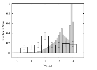
Figure 5: The distribution of $\log g$ in CEMP stars taken from our default stellar population model A (filled histogram) vs our CEMP selection from the SAGA database (open histogram with Poisson error bars).
Note that in this and the similar plots that follow the area under the graph (which is the total number of stars) is normalized such that it is the same for both the observations and our model stars.

In Fig. 5 we compare the distribution of $\log g$ in model set A CEMP stars to our selection from the SAGA database (see Fig. 3b). It is hard to understand why the distributions differ without invoking selection effects such that low-gravity CEMP giants are preferred (see Section 3). We have made no attempt to model such selection effects but we do not expect this to strongly affect our model predictions. The $\log g$ distribution of non-CEMP stars in model set A has a nearly identical shape to the CEMP stars, so that the CEMP/EMP ratio for our default population is independent of $\log g$ and hence the overall CEMP fraction presented in Table 3 is quite robust. We also find that, at least in our default model as well as other models that include thermohaline mixing of accreted material, there is little surface abundance evolution in our CEMP stars after accretion (with the exception of nitrogen, which increases somewhat at first dredge up) so that the abundance distributions we present in the following subsections are also hardly affected by this selection bias.

Finally, we note that the peak in the model distribution at $\log g\sim 3.2$ is due to horizontal branch stars, most of which have effective temperatures close to $10,\!000\,\mathrm{K}$ in our models. The SAGA database does not contain horizontal branch stars hotter than $\sim 7,\!000\,\mathrm{K}$ probably because hotter stars are selected against. If we select only red horizontal branch stars cooler than $7,\!000\,\mathrm{K}$ a small peak at $\log g\sim 2$ remains. This may correspond to the tentative peak seen in the observed distribution.

4.1.3 Carbon, nitrogen and fluorine

The distribution of carbon in the CEMP population of model set A matches reasonably well the observed distribution, as shown in Fig. 6.

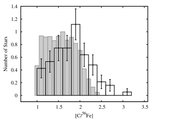
Figure 6: The distribution of $[\mathrm{C}/\mathrm{Fe}]$ in our default CEMP population (model set A, filled histogram) compared to observations (open histogram with Poisson error bars).

The observed distribution shows somewhat higher carbon enhancements on average, while our models predict more stars in the range $1\lesssim[\mathrm{C}/\mathrm{Fe}]\lesssim 1.5$ and none above $[\mathrm{C}/\mathrm{Fe}]=2.5$, compared to about ten observed (11 per cent of the sample). This may be partly explained by our assumption of complete thermohaline mixing: we assume the entire star mixes, when in reality only a fraction mixes.

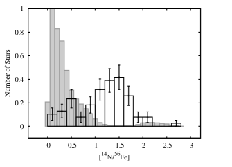
Figure 7: The distribution of $[\mathrm{N}/\mathrm{Fe}]$ in our default CEMP population A (filled histogram) compared to observations (open histogram with Poisson error bars).

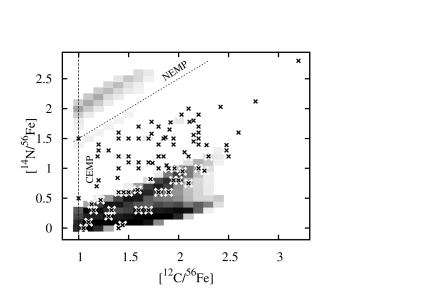
Figure 8: The distribution of $[\mathrm{N}/\mathrm{Fe}]$ versus $[\mathrm{C}/\mathrm{Fe}]$ in our default CEMP population, model set A (darker grey indicates a larger density of stars). The vertical dashed line indicates our CEMP selection criterion ($[\mathrm{C}/\mathrm{Fe}]\geq 1$) and the diagonal dashed line shows our NEMP selection criteria ($[\mathrm{N}/\mathrm{Fe}]\geq 1$ and $[\mathrm{N}/\mathrm{C}]>0.5$). Observed CEMP stars are indicated by crosses.

The picture becomes much less favourable when we compare the distribution of nitrogen, as shown in Figs. 7 and 8. Our default population contains few (C)NEMPs (above the dashed line in Fig. 8; note that NEMPs with $[\mathrm{C}/\mathrm{Fe}]<1.0$ are not shown in this figure), which agrees with both our observational sample and that of Johnson et al. (2007). However, most observed CEMP stars are enhanced in nitrogen by $1-1.5\,\mathrm{dex}$, which in fact coincides with a dearth of model CEMP stars. Our model includes three mechanisms for increasing the nitrogen abundance: first dredge up, hot-bottom burning and third dredge up of the hydrogen burning shell. The latter is only a small effect and while first dredge up enhances $[\mathrm{N}/\mathrm{Fe}]$ by typically $0.5\,\mathrm{dex}$, this cannot reproduce the $1\,\mathrm{dex}$ nitrogen enhancements seen in our observational sample. On the other hand, hot-bottom burning converts most of the dredged-up carbon into nitrogen and thus results in much larger nitrogen enhancements. If HBB were more effective than we assume it would only raise the number of (C)NEMP stars, in contradiction with the observations. We must therefore assume that either some kind of extra-mixing mechanism or a dual core/shell flash is responsible. This is beyond the scope of our present model.

Another indication of a missing ingredient in our models comes from the carbon isotopic ratio. The ${}^{12}\mathrm{C}/\mathrm{{}^{13}}\mathrm{C}$ ratio in our models is always large ($10^{2}-10^{4}$), whereas the observed ratio is generally less than the solar ratio (around 90), from the equilibrium value of four up to about $50$ (Ryan et al., 2005). Again, this may result from extra mixing or a dual shell/core flash.

Figure 9: The distribution of $[\mathrm{F}/\mathrm{Fe}]$ versus $[\mathrm{C}/\mathrm{Fe}]$ in our model set A. The horizontal dashed line indicates our FEMP selection criterion ($[\mathrm{F}/\mathrm{Fe}]\geq 1$) and the vertical dashed line indicates our CEMP selection criterion ($[\mathrm{C}/\mathrm{Fe}]\geq 1$). The position of the fluorine-rich CEMP star HE 1305+0132 is also plotted.

Fluorine was recently measured in the CEMP star HE 1305+0132 (Schuler et al., 2007) and the halo planetary nebula BoBn 1 (Otsuka et al., 2008). Lugaro et al. (2008) pointed out that fluorine is made in the progenitors of CEMP stars and therefore that most CEMP stars should be FEMP stars (EMP stars with $[\mathrm{F}/\mathrm{Fe}]\geq 1$). Fig. 9 confirms this for model set A. Our model struggles to reproduce the $[\mathrm{F}/\mathrm{Fe}]$ ratio of HE 1305+0132 although this star may represent the tail of the fluorine distribution. Future observations of fluorine in CEMP stars should reveal this population. Also, the abundance may be overestimated (Abia et al., 2009).

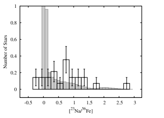
Figure 10: Sodium distribution in our default model set A (filled histogram) compared to observations (open histogram with Poisson error bars).

4.1.4 Sodium and other light elements

Sodium is enhanced at the surface of TPAGB stars through both third dredge up and hot-bottom burning. In our model set A most stars dredge up little sodium, leading to the peak at $[\mathrm{Na}/\mathrm{Fe}]\sim+0$ in Fig. 10. A few of our stars, with relatively massive AGB primaries, dredge up enough sodium that the secondary reaches up to $[\mathrm{Na}/\mathrm{Fe}]\sim 1.5$. The most massive AGB primaries undergo HBB and give rise to the small peak seen at $[\mathrm{Na}/\mathrm{Fe}]\sim 2-2.5$: these stars are CNEMP stars. Our model at least matches the range of observed stars, although sodium-enriched stars are greatly underrepresented. Note that there is great uncertainty in the yield of sodium from massive AGB stars, and hence in our model CNEMP sodium abundances, because of reaction rate uncertainties (Izzard et al., 2007).

Observations of CEMP stars show an overabundance of oxygen and other $\alpha$-elements typical of the halo, i.e. about $+0.4\,\mathrm{dex}$. Our models include no explicit $\alpha$-enhancement but do show enhancements in oxygen and magnesium because of third dredge up (up to $+0.5\,\mathrm{dex}$ and $+0.6\,\mathrm{dex}$ respectively). The few observations of oxygen in CEMP stars range from $0$ to $+2\,\mathrm{dex}$ while magnesium is enhanced by up to $+1.5\,\mathrm{dex}$. It is clear that our models struggle to reproduce these stars, especially because they are often giants which should be well mixed.

There have been several recent lithium abundance measurements in CEMP stars (see e.g. Thompson et al., 2008 and Roederer et al., 2008). Modelling lithium nucleosynthesis is too complicated for our synthetic models. Detailed discussions can be found in Roederer et al. (2008) and Stancliffe (2009).

4.1.5 The heavy elements

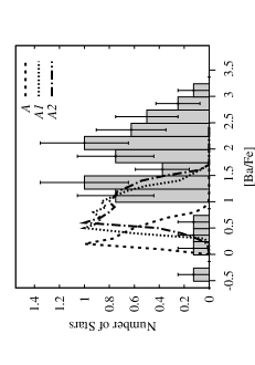
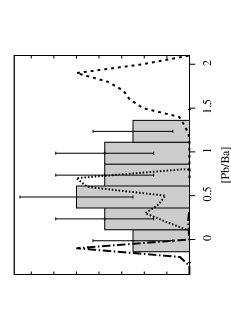
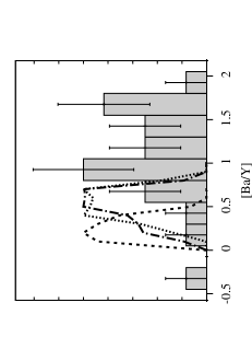
Figure 11: Heavy elements in CEMP stars from model sets A, A1 and A2 with the ${}^{13}\mathrm{C}$ efficiency parameter $\xi_{13}=1$, $0.1$ and $0.01$ respectively. Our observational sample is shown by the filled histograms (with Poisson error bars) while the model sets A, A1 and A2 are plotted with long-dashed, short-dashed and dot-dashed lines respectively. The distributions are all normalized to peak at one. We choose Y, Ba and Pb to represent the $s$-process peaks.

Model A yields a CEMP-$s$/CEMP ratio of only 28 per cent, smaller than is observed: of the 47 CEMP stars in our SAGA database selection with both carbon and barium measured 44 have $[\mathrm{Ba}/\mathrm{Fe}]\geq 0.5$ (94%), while Aoki et al. (2007) report an $s$-rich fraction of 80%. All our model CEMP stars are enriched in $s$-process elements, but most stars in this model have $0<[\mathrm{Ba}/\mathrm{Fe}]<0.5$ and are thus not classified as CEMP-$s$. This is because the assumed ${}^{13}\mathrm{C}$ pocket efficiency $\xi_{13}=1$ gives such a high neutron exposure that the $s$-process distribution is pushed to the lead peak (Gallino et al., 1998). A decreased $\xi_{13}$ (model sets A1 and A2) gives larger barium abundances and hence a larger CEMP-$s$ fraction (see Table 3).

The need to decrease the ${}^{13}\mathrm{C}$ efficiency at low metallicity, to $\xi_{13}\sim 0.1$ for $[\mathrm{Fe}/\mathrm{H}]<-1$, was shown by Bonačić Marinović et al. (2007) on the basis of $[\mathrm{Pb}/\mathrm{hs}]$ ratios in lead stars. A comparison between model set A and the observed heavy element abundance distribution is shown in Fig. 11. We find a best match to the $[\mathrm{Pb}/\mathrm{Ba}]$ ratio for model A1 with $\xi_{13}=0.1$. Although it is unsatisfactory that both the CEMP-$s$ to CEMP ratio and the $s$-abundance ratio distributions depend quite sensitively on a free parameter in the model, we find a reasonable match to all these constraints for a single value of $\xi_{13}$.

4.1.6 Orbital periods

Comparison of observed CEMP orbital periods with our models is difficult for two reasons. First, the number of stars with known periods is small despite the fact that many are binaries – from our selection there are only six stars with orbital solutions (see Table 4). Second, long periods are difficult to measure. Any period longer than about ten years, which is approximately the time for which surveys have been ongoing, is likely to remain unmeasured for some time to come. With this in mind, Figure 12 shows the distribution of periods from model set A compared to the six observed stars.

Object	Period	$e$	Reference
CS22948-027	505d	0.3	Preston & Sneden (2001)
CS22948-027	426.5d	0.02	Barbuy et al. (2005)
HD5223	755.2d	0	McClure & Woodsworth (1990)
HD224959	1273d	0.179	McClure & Woodsworth (1990)
CS22956-028	1290d	0.22	Sneden et al. (2003)
CS22942-019	2800d	0.19	Preston & Sneden (2001)
LP 625-44	12y		Aoki et al. (2000)

Table 4: Periods and eccentricities of CEMP stars in binaries from our selection ($[\mathrm{Fe}/\mathrm{H}]=-2.3\pm 0.5$, $\log_{10}g\leq 4$). Note that two solutions are available for CS22948-027.

Figure 12: Period distribution in our CEMP model sets A, G and H (solid lines, dashes and dot-dashes respectively) vs CEMP period measurements from our selection of the SAGA database (crosses).

The lower limit to the model period distribution is set by systems that are just wide enough for the AGB primary to avoid filling its Roche lobe when the star has its maximum radius. The shortest-period CEMP binaries, CS22948-027 and HD5223, are not compatible with our model set A. Their short periods and small eccentricities (if we adopt the Barbuy et al., 2005 result regarding CS22948-027) suggest they underwent tidal circularisation, and perhaps RLOF and common-envelope evolution. This does not explain their carbon enhancement. The problem is reminiscent of the barium stars, which have too large eccentricities and too short periods compared to models (Pols et al., 2003). Various explanations have been proposed to deal with this problem which build on the fact that AGB stars have very extended, outflowing atmospheres such that the canonical distinction between RLOF (when the stellar surface fills the Roche lobe) and wind accretion (when it does not) becomes blurred (e.g. see Frankowski & Jorissen, 2007, Bonačić Marinović et al., 2008). Our understanding of binary evolution in this transition region is still poor. An alternative solution may be accretion during the common-envelope phase (Ricker & Taam, 2008), which we explore in model H (see Section 4.2).

The remaining stars, HD224959, CS22956-028, CS22942-019 and LP 625-44, all lie at the short-period end of the range produced by our model set A, as is to be expected from the above-mentioned selection effects.

4.2 Model sets G and H: best comparison to observations

The discussion of the previous section suggests that to better match our models with the observations we should consider an increase in the amount of third dredge up in low mass stars and the effect of switching off thermohaline mixing. To this end we consider model sets G and H.

4.2.1 Model set G: extra third dredge up

Model sets E, F and G are the same as our default set (set A) except that third dredge up is increased in efficiency in low mass stars. In model E we have set $\Delta M_{\mathrm{c},\mathrm{min}}=-0.07\mathrm{\,M_{\odot}}$ and $\lambda_{\mathrm{min}}=0.8$, which is the set of values found by Izzard et al. (2004) to be required to match the carbon-star luminosity functions of the Magellanic Clouds. This results in only a modest increase of the number of CEMP stars, see Table 3. A larger effect is obtained by setting $\Delta M_{\mathrm{env},\mathrm{min}}=0.0$ in model F, which allows for efficient dredge-up in AGB stars of much smaller initial masses and increases the CEMP/EMP ratio to 6.5 per cent. Model G is a combination of these parameter choices with $\Delta M_{\mathrm{c},\mathrm{min}}=-0.1\mathrm{\,M_{\odot}}$. With this parameter combination all primary TPAGB stars down to initial masses of $0.8\mathrm{\,M_{\odot}}$ undergo efficient third dredge up. The IMF peaks at low mass, so the number of stars affected is large and the CEMP/EMP ratio increases to almost $10\%$ – a factor of four increase compared to our default models. The NEMP/EMP ratio remains small at $0.3\%$.

Figure 13: Model set G: a $[\mathrm{N}/\mathrm{Fe}]$ vs $[\mathrm{C}/\mathrm{Fe}]$ and b $[\mathrm{Pb}/\mathrm{Fe}]$ vs $[\mathrm{Ba}/\mathrm{Fe}]$. Crosses show our observational sample. This model set is the same as our default set (model set A) but with efficient third dredge up in stars down to $0.8\mathrm{\,M_{\odot}}$ and a reduced ${}^{13}\mathrm{C}$ efficiency.

The distribution of $[\mathrm{C}/\mathrm{Fe}]$ reaches up to $+2.7$ and is in good agreement with the observations (see Fig. 13a). The distributions of nitrogen (Fig. 13a) and sodium suffer the same problems as in the default model set. Although the total amount of $\mathrm{C}+\mathrm{N}$ (and hence the total amount of third dredge up) as well as the observed trend of $[\mathrm{N}/\mathrm{Fe}]$ vs $[\mathrm{C}/\mathrm{Fe}]$ roughly match the observations, there is clearly a need for some additional CN cycling to convert carbon into nitrogen.

Model set G has a reduced ${}^{13}\mathrm{C}$ efficiency, $\xi_{13}=0.1$ as in model A1. This yields a reasonably good fit to the observations for the light-$s$ elements strontium, yttrium and zirconium, but the stars most strongly enriched in heavy-$s$ elements such as barium (with $[\mathrm{Ba}/\mathrm{Fe}]>+2.7$) are not well reproduced. Fig. 13b reveals that, firstly, our models predict a strong correlation between barium and carbon (as well as between other $s$-process elements) which is not seen. The spread in the observations is only partially explained by measurement errors. Secondly, the models trace out roughly the lowest observed barium abundances for any value of $[\mathrm{C}/\mathrm{Fe}]$. More barium can be produced in our models by further reducing the ${}^{13}\mathrm{C}$ efficiency, as discussed in Section 4.1.5, but only at the expense of lead. With the adopted value of $\xi_{13}$ the average observed barium to lead ratio is well matched, although the most lead-rich stars (with $[\mathrm{Pb}/\mathrm{Fe}]>+2.7$) are not reproduced. The CEMP-$s$/CEMP ratio for this model set is $94\%$, in agreement with observations.

Interestingly, some CEMP binaries are made in model set G which have periods of one to a few years, similar to the observed short-period giant CEMP stars (see Fig. 12). These arise from binaries with low-mass AGB primaries which have smaller maximum radii and can thus avoid filling their Roche lobes in tighter orbits. Because the initial mass ratio is close to unity and the primary may even be less massive than the secondary due to mass loss prior to the AGB, these binaries may also undergo stable RLOF without a common envelope phase.

4.2.2 Model set H: extra third dredge up, no thermohaline mixing, common envelope accretion

Model set H is similar to G, as described in the previous section, but is tuned to maximise the CEMP/EMP ratio. Thermohaline mixing is turned off so that accreted material remains in the surface convection zone. Before the star ascends the giant branch and its convection zone deepens, its surface composition is therefore essentially the same as that of the primary TPAGB star ejecta. Furthermore, during the common envelope phase accretion of $0.05\mathrm{\,M_{\odot}}$ of material is allowed, so some stars that undergo RLOF can become CEMP stars. These changes mean that CEMP stars can form out to longer periods and more turn-off stars and subgiants, with $\log g\gtrsim 3.5$, become CEMP stars because there is no dilution until first dredge up. While the individual effects of these changes on the number of CEMP stars are modest (see models C and D in Table 3), in combination with extra third dredge-up they yield a CEMP/EMP ratio of almost $16\%$.

Figure 14: As Fig. 13 for model set H.

The effect on our model abundance distributions is significant: the sub-giant and turn-off CEMP stars form a group of stars with undiluted abundances. In the case of $[\mathrm{C}/\mathrm{Fe}]$ these are between $+3$ and $+4\,\mathrm{dex}$ (see Fig. 14a), which does not match the observations – only one star in our observed selection has $[\mathrm{C}/\mathrm{Fe}]=+3$ and none are more enhanced than this. It may be argued that this excess carbon is converted to nitrogen by extra mixing processes, but then $[\mathrm{N}/\mathrm{Fe}]$ should rise to approximately $+3\,\mathrm{dex}$ in some stars, which is not observed either. Our model $[\mathrm{N}/\mathrm{Fe}]$ distribution ranges up to $+2\,\mathrm{dex}$, as do most of the observations, but while in our model these correspond to the most C-enriched, undiluted stars, the observed nitrogen-rich stars have more modest carbon enhancements.

The undiluted turn-off stars in model H result in a peak in the sodium distribution at around $0.8\,\mathrm{dex}$, in better agreement with the (broad) peak in the observations than our models with thermohaline mixing. Similarly, a broad distribution of oxygen abundances is obtained, out to about $+1.7\,\mathrm{dex}$, also in better agreement with the observations.

The heavy element distributions are reasonably well matched by this model, although the maximum abundances predicted (for undiluted stars) are sometimes in excess of what is observed. This is especially true for the light-$s$ elements, for which this model set makes too many stars with large enhancements (up to $+2.5\,\mathrm{dex}$ for $[\mathrm{Zr}/\mathrm{Fe}]$ and$+2.2\,\mathrm{dex}$ for $[\mathrm{Y},\,\mathrm{Sr}/\mathrm{Fe}]$) which are not seen in the observations. Lanthanum and barium are enriched up to $+3.2\,\mathrm{dex}$ in this model which is in agreement with observations, although the most barium-rich objects have too much carbon (see Fig. 14b). The models cover the full range of lead observations, up to $\sim 3.5\,\mathrm{dex}$.

We must keep in mind that the undiluted stars in our models, which have the largest overabundances for all the elements discussed above, are also high-gravity stars against which there is an apparent observational bias (see Sections 3 and 4.1.2). They may therefore be overrepresented in our model distributions compared to the observational samples. We also note that in our observational selection, no correlation of the abundance distributions against $\log g$ is apparent for any of the elements discussed above. However, Denissenkov & Pinsonneault (2008) and Aoki et al. (2008) do find evidence for significantly higher average $[\mathrm{C}/\mathrm{Fe}]$ values in turn-off CEMP stars compared to bright giants.

This model set also includes accretion of up to $0.05\mathrm{\,M_{\odot}}$ of material during the common envelope phase. This allows CEMP formation in the narrow range of initial separation corresponding to primary TPAGB stars which undergo a few pulses before overflowing their Roche lobe, and leads to a peak in the orbital period distribution around one year and a tail extending down to $100\,\mathrm{days}$ (see Fig. 12). This is just the range which includes the stars described in Section 4.1.6 and may explain their origin.

4.3 Model set conclusions

It appears from the previous sections that our models struggle to reproduce both the observed frequency of CEMP stars and the full range of their abundance patterns. Unless we choose a rather extreme combination of model parameters our model CEMP/EMP ratio falls short of the range of values deduced from observations and does not exceed $16\%$ even in our most favourable model.

In order to come close to reproducing the observations, we must assume that TPAGB stars with masses as low as $0.8\mathrm{\,M_{\odot}}$ experience efficient third dredge up. This yields a good fit of the distribution of carbon enhancements, but still falls short of reproducing the largest observed $s$-process abundances. If we switch off thermohaline mixing we find, on the other hand, that the $s$-process elements are quite well reproduced, but our model CEMP stars have too much carbon (and perhaps also lead). We note that both the $s$-process abundance ratios and the CEMP-$s$/CEMP ratio depend on the ${}^{13}\mathrm{C}$ pocket efficiency. We can find a reasonable match to these constraints by choosing this efficiency to be about 0.1 times its default value.

The orbital periods of CEMP binaries in our observational sample agree well with the shortest period CEMP stars in both these model sets, so it seems that – at least for the few systems with measured periods – the binary mass-transfer scenario is compatible with the observations.

5 Discussion

We have modelled the observed properties – $\log g$, chemistry and orbital period – of CEMP stars and have attempted to match our models to observed stars. Our models are successful in reproducing several key observed properties of CEMP stars, but struggle to match the full range of the observations, most notably the high CEMP fraction, even with rather extreme choices of model parameters.

The first criticism that can be levelled at our work is probably our choice of stars from, and subsequent processing of, the SAGA observational database. We chose a group of stars limited by metallicity, $[\mathrm{Fe}/\mathrm{H}]=2.3\pm 0.5$, because our stellar models have $Z=10^{-4}$. As shown in Section 3, the statistics (number of stars, CEMP/EMP ratios etc.) of our selection vary remarkably little as a function of $[\mathrm{Fe}/\mathrm{H}]$ so the selection is justified in this respect. However, there may be a selection effect inherent in the SAGA database because papers are selected for inclusion in it if they contain stars with $[\mathrm{Fe}/\mathrm{H}]\leq-2.5$. Stars with higher metallicities, of which there are many in the database, are included because they just happen to be in those papers.

We should then consider the selection criterion $\log g\leq 4$. While we select identically in the models it is reasonable to ask which model constraints are weakened by this choice. The answer is few: most stars in the SAGA database are giants. This is also the result of a bias against faint, high-gravity stars that is inherent in the SAGA database. We have made no attempt to model such a selection bias in any detail and our simple gravity criterion is not entirely successful in selecting against turn-off stars which may be affected by the uncertain strength of thermohaline mixing. On the other hand, giants are well mixed as their surface convection zones deepen on the giant branch and so whether we assume efficient thermohaline mixing, or do not, is of minor importance provided we look only at giants and avoid elements which may be processed in the envelope (see e.g. Stancliffe & Glebbeek, 2008 and Stancliffe, 2009).

The exception to this rule lies with carbon and nitrogen. The amount of nitrogen dredged up as the convection zone deepens depends on whether accreted carbon has mixed deep enough to be burned by the CN cycle. In the case of efficient thermohaline mixing this is certainly the case, although to some extent the dilution associated with such deep mixing reduces the effect of first dredge up. On the other hand, if accreted carbon sits at the stellar surface it does not burn to nitrogen. Almost all the nitrogen seen in the CEMP star must then come from the primary star, posing the questions of whether extra mixing, dual-shell flashes and dual-core flashes are important. Interesting progress is being made regarding these questions (e.g. Stancliffe et al., 2009).

We have tried to push the physics of the canonical third dredge up as far as possible, inducing it in stars down to $0.8\mathrm{\,M_{\odot}}$ with large efficiency. Previous models suggest that stars with envelope masses less than $0.5\mathrm{\,M_{\odot}}$ do not undergo third dredge up, although many of these models are for higher metallicity than we are considering here.

Stancliffe & Glebbeek (2008) have made a model of a $0.9\mathrm{\,M_{\odot}}$ star with $Z=10^{-4}$ which does undergo third dredge up. The efficiency is not high, $\lambda=0.16$, but carbon is dredged to the surface. At the time that third dredge up occurs the star has an envelope mass of just $0.19\mathrm{\,M_{\odot}}$ and the dredge up is sufficient to increase the surface carbon abundance dramatically, from just $6\times 10^{-6}$ up to $3.7\times 10^{-3}$ by mass fraction.

If third dredge up is as efficient as assumed in our models that provide the best match to observations we would expect to see a population of (single) CEMP stars that are currently in the TPAGB phase with $\log g<0.5$. Masseron et al. (2006) have suggested that CS 30322-023 is just such a star. They construct a $0.8\mathrm{\,M_{\odot}}$, $[\mathrm{Fe}/\mathrm{H}]=-3.3$ detailed model sequence with the starevol code (Siess, 2006) for comparison with observations of CS 30322-023. They find no third dredge up, which is not surprising given that models constructed with starevol do not show third dredge up unless some kind of neutral-convective-boundary method or overshooting is invoked. However the authors make clear our lack of quantitative understanding of mixing processes in these stars. Other mechanisms such as dual shell and/or core flashes, proton ingestion and so-called “canonical” extra mixing may, to some extent, mimic the nucleosynthetic signature of third dredge up. At the very least, if CS 30322-023 is a (single) TPAGB star, as Masseron et al. (2006) suggest, it certainly has undergone some nucleosynthetic processing in order to reach $[\mathrm{C}/\mathrm{Fe}]\sim+0.6$ and $[\mathrm{N}/\mathrm{Fe}]\sim+2.8$. Convective overshooting may also play a role in enhancing third dredge up in low-mass stars: prescriptions such as that of Herwig (2000) contain free parameters which have the same effect as our $\Delta M_{\mathrm{c},\mathrm{min}}$ and $\lambda_{\mathrm{min}}$.

Even with enhanced third dredge up efficiency our models barely make enough CEMP stars to match the observed fraction. There are more exotic methods for increasing the number of CEMP stars. One is to accrete material from a TPAGB star on to a main-sequence star during the common-envelope phase which should occur for most TPAGB primaries that overflow their Roche lobe. We assumed $0.05\mathrm{\,M_{\odot}}$ is accreted on to the main-sequence star, which is probably too much (Ricker & Taam, 2008), so gives an upper limit. In any case, if there is no thermohaline mixing in the main-sequence star even a tiny amount of accreted carbon-rich material should turn it into a CEMP star. Still, even with $0.05\,\mathrm{M}_{\odot}$ of accreted material, only a few extra CEMP stars are made. This is because the period range in which AGB stars both have enough pulses to become carbon rich and then undergo RLOF is rather narrow. At a slightly smaller period RLOF occurs too early, i.e. after too few (or no) third dredge up episodes and little or no carbon enhancement.

We also considered a reduction in the common-envelope parameter such that $\alpha_{\mathrm{CE}}=0.1$. This does not increase the number of CEMP stars – instead it reduces the number of non-CEMP stars by forcing many short-period systems to merge. After the merger the stellar mass is so large that the star evolves quickly and by the present age of the Galaxy it is a white dwarf. We do not pretend that this mechanism is realistic, but it may help to improve the CEMP/EMP ratio match with observations.

A non-canonical dredge up event may lead to the formation of CEMP (and possibly NEMP) stars. Previous works, such as Komiya et al. (2007), have suggested that below a certain threshold metallicity, in their work $[\mathrm{Fe}/\mathrm{H}]=-2.5$, dual shell flashes make all the required nitrogen and some of the carbon and $s$-process elements seen in CEMP stars. The recent works of Cristallo et al. (2007) and Campbell & Lattanzio (2008) indeed show some agreement with the observed carbon and nitrogen abundances. However, at the metallicity under consideration here ($[\mathrm{Fe}/\mathrm{H}]\sim-2.3$) these proton-ingestion events are not expected to occur – or at least only in the lowest mass stars – and the number of CEMP stars should drop as the metallicity increases. Extra mixing processes, and a dependence on stellar properties other than the metallicity, may well blur the apparently sharp boundary between stars that undergo dual-shell flashes and those that do not. Incorporation of the results of Cristallo et al. (2007) and Campbell & Lattanzio (2008) into our models is planned for future work.

A deliberate omission in the above is discussion of the binary fraction in low-metallicity stars. In order to obtain anywhere near the observed CEMP fraction we must assume a $100\%$ binary fraction. This should be compared to about $60\%$ in solar-neighourhood G dwarfs (Duquennoy & Mayor, 1991) and probably higher among stars more massive than the Sun.

We are left with the situation that in order for our models to come close to reproducing the observed CEMP/EMP fraction several physical parameters must be pushed to the ends of their reasonable range of values. This is not a very satisfactory solution, and probably indicates that other phenomena require our consideration, such as a shift in the initial mass function (Komiya et al., 2007; Lucatello et al., 2006), massive-star pollution, primordial supernovae, accretion from the interstellar medium etc. All of these solutions to reproducing the CEMP/EMP fraction have their own problems. Most likely, some combination of our physical models with, say, a slightly-shifted IMF (or other initial distribution), will better reproduce the CEMP/EMP fraction. Our investigation into this is ongoing and will comprise future work.

Finally, we note that both the observational statistics and the observed abundances of CEMP stars are still uncertain. Interesting results regarding three-dimensional stellar atmosphere models (Collet et al., 2007) may be of relevance to CEMP studies. They conclude that the abundances of C, N and O in red giants with metallicity $[\mathrm{Fe}/\mathrm{H}]=-3$ may be overestimated by up to $1\,\mathrm{dex}$ in traditional one-dimensional LTE model atmosphere analyses. If we apply these corrections to the Suda database, with the crude assumption of a linear scaling as a function of metallicity, the resulting CEMP/EMP ratio drops to about $14\%$ which well fits our enhanced dredge up models. We are not suggesting this is the answer to the CEMP/EMP ratio problem, but it highlights the fact that observed carbon and nitrogen abundances, and hence CEMP number counts, are still quite uncertain.

6 Conclusions

In an attempt to reproduce the observed CEMP to EMP number ratio we have simulated populations of low-metallicity ($[\mathrm{Fe}/\mathrm{H}]=-2.3$) binary stars with a variety of input physics. Our model sets with efficient third dredge up in low-mass (down to $0.8\mathrm{\,M_{\odot}}$) stars have CEMP to EMP ratios of up to $15\%$, comparable with the observed $\sim 20\%$. They also have low NEMP to EMP number ratios, in agreement with the observations. Other parameters in our simulations, such as the efficiency of wind accretion, the common envelope parameter etc., have only relatively minor effects on our results.

Appendix A Dredge Up Prescriptions

A.1 First dredge up

The change in surface abundance of isotopes $j$ at first dredge up, $\Delta X_{j}$, is interpolated from a table of detailed models with $Z=10^{-4}$ in mass range $0.5\leq M/\mathrm{M_{\odot}}\leq 12$. A correction factor $f_{\mathrm{CNO}}=X_{\mathrm{CNO}}(\mathrm{TMS})/X_{\mathrm{CNO}}(\mathrm{ZAMS})$, the ratio of CNO mass fraction at the terminal-age main sequence (TMS) and zero-age main sequence (ZAMS), is then applied to CNO elements to take into account accretion during the main sequence.

In the Izzard et al. (2006) model first dredge up is considered as an instantaneous event. In terms of time evolution this is a reasonable assumption because giant-branch evolution is fast, but in terms of luminosity or gravity this approximation is not good and it proves difficult to compare to e.g. the $[\mathrm{C}/\mathrm{Fe}]$ vs $\log\left(L/\mathrm{L_{\odot}}\right)$ data of Lucatello et al. (2006). To resolve this problem the changes in abundances are modulated by a factor $f_{\mathrm{p}}=\min\left[\left(M_{\mathrm{c}}-M_{\mathrm{c,BAGB}}\right)/\left(M_{\mathrm{c,1DUPMAX}}-M_{\mathrm{c,BAGB}}\right),1\right]$ where $M_{\mathrm{c}}$ is the core mass, $M_{\mathrm{C,1DUPMAX}}$ is the core mass at which first dredge up reaches its maximum depth and $M_{\mathrm{c,BAGB}}$ is the core mass at the base of the giant branch, before first dredge up starts. $M_{\mathrm{c,BAGB}}$ is known from the stellar evolution prescription and $M_{\mathrm{C,1DUPMAX},}$ is interpolated from a grid of models constructed with the TWIN stellar evolution code (Eggleton & Kiseleva-Eggleton, 2002).

In summary, the surface abundances changes at first dredge up are given by $f_{\mathrm{CNO}}f_{\mathrm{p}}\Delta X_{j}$. They agree well with the detailed models, as a function of $M_{\mathrm{c}}$, $\log L$ and time.

A.2 Third dredge up

Abundance changes at third dredge up are treated in a similar way to the prescription of Izzard et al. (2004) and Izzard et al. (2006). Intershell abundances are interpolated from tables based on the Karakas et al. (2002) detailed models the metallicities of which extend down to $Z=10^{-4}$.

In low-metallicity TPAGB stars dredge up of the hydrogen-burning shell enhances the surface abundance of ${}^{13}\mathrm{C}$ and ${}^{14}\mathrm{N}$ (at higher metallicity the effect is negligible because the initial abundance of ${}^{13}\mathrm{C}$ and ${}^{14}\mathrm{N}$ is relatively large). This is modelled by dredging up $\delta M$ of hydrogen-burnt material during each third dredge up, where the abundance mixture in this material is enhanced in ${}^{13}\mathrm{C}$ and ${}^{14}\mathrm{N}$ according to

$$X_{\mathrm{C}13} = 0.006\times X_{\mathrm{C}12}\,\mathrm{and}$$ (3)

$$X_{\mathrm{N14}} = 0.28\times X_{\mathrm{C}12}\,,$$ (4)

where

$$\delta M = \left(\frac{0.01}{1+0.1^{2.2-M(t)}}\right)\times\min\left(1,\left[\frac{N_{\mathrm{TP}}}{10}\right]^{2}\right)\times$$ (5)

$$\left(\frac{1}{1+\epsilon^{M_{\mathrm{env}}(t)-0.5}}\right)$$

and $M(t)$ is the instantaneous stellar mass, $M_{\mathrm{env}}(t)$ is the instantaneous envelope mass, $N_{\mathrm{TP}}$ is the thermal pulse number, $X_{12}$ is the envelope abundance of ${}^{12}\mathrm{C}$ and $\epsilon=10^{-20}$. The first term gives the amount of H-burnt material dredged up, the second term is a turn-on effect as the star reaches the asymptotic regime and the third term is a turn-off effect for small envelopes.

Appendix B Mass-loss prescriptions

We consider three mass-loss prescriptions for TPAGB stars.

VW93

The formalism of Vassiliadis & Wood (1993, VW93) relates the mass-loss rate to the Mira pulsation period of the star, given by

$$P_{0} = 10^{-2.07-0.90L/\mathrm{L_{\odot}}+1.94\log_{10}\left(R/\mathrm{R_{\odot}}\right)}\,\mathrm{days}.$$ (6)

The mass loss rate is then given by, as in Karakas et al., 2002, i.e. without the $M/\mathrm{M_{\odot}}-2.5$ term of the original VW93 prescription,

$$\dot{M}=\dot{M}_{\mathrm{VW0}} = f_{\mathrm{VW}}\left(-11.4+0.0125P_{0}\right)\mathrm{\,M_{\odot}}\,\mathrm{yr}^{-1}$$ (7)

unless $P_{0}>\left(500-\Delta P_{\mathrm{VW}}\right)\,\mathrm{days}$ in which case a superwind is applied

$$\dot{M} = \max\left(\dot{M}_{\mathrm{VW0}},f_{\mathrm{VW}}\frac{Lc}{v_{\mathrm{w}}}\right)$$ (8)

where

$$v_{\mathrm{w}} = 10^{5}\left(-13.5+0.056P_{0}\right)\,\mathrm{cm}\,\mathrm{s}^{-1}\,.$$ (9)

The free parameters $f_{\mathrm{VW}}$ and $\Delta P_{\mathrm{VW}}$ subtly affect the mass-loss rate. The factor $f_{\mathrm{VW}}$ is a simple multiplier, which is $1$ by default (see model set 27). The period shift $\Delta P_{\mathrm{VW}}$ allows the onset of the superwind to be delayed, e.g. $\Delta P_{\mathrm{VW}}=-100\,\mathrm{days}$ in model set 33 – it is zero by default.

Reimers

The Reimers mass-loss rate is given by

$$\dot{M} = 4\times 10^{-13}\eta\frac{RL}{M}\mathrm{\,M_{\odot}}\,\mathrm{yr}^{-1}\,,$$ (10)

where $\eta$ is a parameter of order unity (Reimers, 1975) which we vary in model sets 10, 11 and 12.

van Loon

In model set 13 we use the split form of van Loon et al. (2005) appropriate to oxygen-rich red giants,

$$\log_{10}\left[\dot{M}/(\mathrm{M_{\odot}}\mathrm{yr}^{-1})\right] =$$

$$\mbox{}{\left\{\begin{array}[]{cc}-5.6+1.10l_{4}-5.2\mathrm{t_{35}}&l_{4}<0.9\,\mathrm{and\,}\\ -5.3+0.82l_{4}-10.8t_{35}&l_{4}\geq 0.9\,,\end{array}\right.}$$ (13)

where $l_{4}=\log_{10}\left(L/10^{4}\mathrm{L_{\odot}}\right)$ and $t_{\mathrm{35}}=\log_{10}\left(T_{\mathrm{eff}}/3500\mathrm{K}\right)$. Note, if $T_{\mathrm{eff}}>4000\,\mathrm{K}$ we enforce a minimum mass-loss rate of $10^{-4}\mathrm{\,M_{\odot}}\,\mathrm{year}^{-1}$ because the above formula can approach zero as the temperature rises (and the envelope mass becomes small) as a star approaches the white-dwarf cooling track.

Appendix C Binary distributions

Our default binary-star distribution is the combination of

1. The initial mass function (IMF) of Kroupa et al. (1993, KTG93) for the initial primary mass $M_{1}$

   $$\psi(M_{1})=\left\{\begin{array}[]{ll}0&M_{1}/\mathrm{\,M_{\odot}}\leq m_{0}\\ a_{1}(M_{1}/\mathrm{M_{\odot})}^{p_{1}}&m_{0}<M_{1}/\mathrm{M_{\odot}}\leq m_{1}\\ a_{2}(M_{1}/\mathrm{M_{\odot})}^{p_{2}}&m_{1}<M_{1}/\mathrm{M_{\odot}}\leq m_{2}\\ a_{3}(M_{1}/\mathrm{M_{\odot}})^{p_{3}}&m_{2}<M_{1}/\mathrm{M_{\odot}}\leq m_{\textrm{max}}\\ 0&m>m_{\textrm{max}}\end{array}\right.$$ (14)

   where $p_{1}=-1.3$, $p_{2}=-2.2$, $p_{3}=-2.7$, $m_{0}=0.1$, $m_{1}=0.5$, $m_{2}=1.0$ and $m_{\textrm{max}}=80.0$. Continuity requirements and $\int\psi(M)dM=1$ give the constants $a_{1}$, $a_{2}$ and $a_{3}$.

2. A distribution flat in $q=M_{2}/M_{1}$ for the initial secondary mass $M_{2}$, where $M_{2}\leq M_{1}$

3. A distribution flat in $\ln a$ (i.e. probability $\sim 1/a$) for the separation $a$ where $3\leq a\leq 10^{5}$.

4. Initially circular binaries (except for model set Ae5).

Appendix D All Model Sets and Results

Table 5 shows the full set of models we considered, of which Table 1 is a subset.

Table 6 shows the full set of CEMP, CNEMP and NEMP to EMP ratios for all our model sets of which Table 3 is a subset.

Model Set	Physical Parameters (differences from model set A)
A	-
CEp1, CE3	$\alpha_{\mathrm{CE}}=0.1$ and $3$ respectively
B	Bondi-Hoyle $\alpha_{\mathrm{BH}}=5$
Ae5	Initial eccentricity $e=0.5$
8	CRAP parameter $B=10^{3}$
E	Third DUP calibration: $\Delta M_{\mathrm{c},\mathrm{min}}=-0.07\mathrm{\,M_{\odot}}$, $\lambda_{\mathrm{min}}=0.8$
10, 11, 12	Reimers AGB wind: $\eta=0.1$, $1$ and $5$ respectively
13	AGB wind of Van Loon
14, 15, C	Common envelope accretion $0.01$, $0.02$ and $0.05\mathrm{\,M_{\odot}}$ respectively
A1, A2	${}^{13}\mathrm{C}$ efficiency parameter $0.1$ and $0.01$ respectively
D	Thermohaline mixing disabled
At12, At8	Minimum CEMP age $12$ and $8\,\mathrm{Gyr}$ respectively
F	Third DUP $M_{\mathrm{env},\mathrm{min}}=0\mathrm{\,M_{\odot}}$
27	$M_{\mathrm{env},\mathrm{min}}=0\mathrm{\,M_{\odot}}$, $\xi_{\mathrm{13}}=0.01$, $\Delta M_{\mathrm{c,min}}=-0.1\mathrm{\,M_{\odot}}$, $\lambda_{\mathrm{min}}=0.5$, $f_{\mathrm{VW}}=0.1$
28	$M_{\mathrm{env},\mathrm{min}}=0\mathrm{\,M_{\odot}}$, $\xi_{\mathrm{13}}=0.01$, $\Delta M_{\mathrm{c,min}}=-0.1\mathrm{\,M_{\odot}}$, $\lambda_{\mathrm{min}}=0.5$
Ap5, Ap7	$\left[\mathrm{C}/\mathrm{Fe}\right]_{\mathrm{min}}=0.5$ and $0.7$ respectively
31, 32	As 27 with $\left[\mathrm{C}/\mathrm{Fe}\right]_{\mathrm{min}}=0.5$ and $0.7$ respectively
33	$\Delta P_{\mathrm{VW}}=-100\,\mathrm{days}$
34, B1	$M_{\mathrm{env},\mathrm{min}}=0\mathrm{\,M_{\odot}}$, $\xi_{\mathrm{13}}=0.01$, $\Delta M_{\mathrm{c,min}}=-0.1\mathrm{\,M_{\odot}}$ with $\lambda_{\mathrm{min}}=0.1$ and $0.8$ respectively
36	$M_{\mathrm{env},\mathrm{min}}=0.25\mathrm{\,M_{\odot}}$, $\xi_{\mathrm{13}}=0.01$, $\Delta M_{\mathrm{c,min}}=-0.1\mathrm{\,M_{\odot}}$, $\lambda_{\mathrm{min}}=0.8$
37, 38, 39, 40	Nelemans common-envelope prescription, $\gamma=0.5$, $1$, $1.5$ and $2$ respectively
41	As 39 but Nelemans prescription for $q>0.2$ only (otherwise the default prescription)
42	As 41 but Nelemans prescription only for the first common-envelope phase
B2	$\alpha_{\mathrm{CE}}=0.1$, $M_{\mathrm{env},\mathrm{min}}=0\mathrm{\,M_{\odot}}$, $\Delta M_{\mathrm{c,min}}=-0.1\mathrm{\,M_{\odot}}$, $\lambda_{\mathrm{min}}=0.5$ , Comenv accretion $0.05$, No thermohaline
44	38 and B2 combined
45	As B1 with $\xi_{\mathrm{13}}=0.1$
48	$M_{\mathrm{env},\mathrm{min}}=0\mathrm{\,M_{\odot}}$, $\Delta M_{\mathrm{c,min}}=-0.1\mathrm{\,M_{\odot}}$, $\lambda_{\mathrm{min}}=0.5$, $\xi_{\mathrm{13}}=0.01$
G	$M_{\mathrm{env},\mathrm{min}}=0\mathrm{\,M_{\odot}}$, $\Delta M_{\mathrm{c,min}}=-0.1\mathrm{\,M_{\odot}}$, $\lambda_{\mathrm{min}}=0.8$, $\xi_{\mathrm{13}}=0.1$
50	$M_{\mathrm{env},\mathrm{min}}=0\mathrm{\,M_{\odot}}$, $\Delta M_{\mathrm{c,min}}=-0.1\mathrm{\,M_{\odot}}$, $\lambda_{\mathrm{min}}=0.5$, $\xi_{\mathrm{13}}=0.001$
51, 52, 53	Comenv accretion $0.05\mathrm{\,M_{\odot}}$, $M_{\mathrm{env},\mathrm{min}}=0\mathrm{\,M_{\odot}}$, $\Delta M_{\mathrm{c,min}}=-0.1\mathrm{\,M_{\odot}}$, $\lambda_{\mathrm{min}}=0.5$, $\xi_{\mathrm{13}}=0.1,\,0.01\,\mathrm{and}\,0.001$ respectively
H, 55, 56	Comenv accretion $0.05\mathrm{\,M_{\odot}}$, $M_{\mathrm{env},\mathrm{min}}=0\mathrm{\,M_{\odot}}$, $\Delta M_{\mathrm{c,min}}=-0.1\mathrm{\,M_{\odot}}$, $\lambda_{\mathrm{min}}=0.8$, $\xi_{\mathrm{13}}=0.1,\,0.01\,\mathrm{and}\,0.001$ respectively
57, 58, 59	$M_{\mathrm{env},\mathrm{min}}=0\mathrm{\,M_{\odot}}$, $\Delta M_{\mathrm{c,min}}=-0.1\mathrm{\,M_{\odot}}$, $\lambda_{\mathrm{min}}=0.5$, $\xi_{\mathrm{13}}=0.1,\,0.01\,\mathrm{and}\,0.001$ respectively

Table 5: The full list of our binary population models (a subset is shown in Table 1). The meanings of the symbols are given in Section 2.

Model Set	CEMP/EMP $\%$	CNEMP/EMP $\%$	NEMP/EMP $\%$
$\emph{A},\emph{A1},\emph{A2}$	$2.300\pm 0.034$	$0.098\pm 0.002$	$0.267\pm 0.007$
CEp1	$2.370\pm 0.029$	$0.100\pm 0.002$	$0.273\pm 0.007$
CE3	$2.300\pm 0.033$	$0.097\pm 0.002$	$0.267\pm 0.006$
B	$3.050\pm 0.038$	$0.157\pm 0.003$	$0.323\pm 0.006$
Ae5	$2.150\pm 0.033$	$0.086\pm 0.002$	$0.249\pm 0.007$
8	$2.460\pm 0.034$	$0.101\pm 0.002$	$0.268\pm 0.006$
E	$2.900\pm 0.040$	$0.098\pm 0.002$	$0.267\pm 0.006$
10	$2.640\pm 0.032$	$0.208\pm 0.003$	$0.310\pm 0.005$
11	$1.490\pm 0.021$	$0.053\pm 0.001$	$0.091\pm 0.002$
12	$0.489\pm 0.009$	$0.005\pm 0.000$	$0.015\pm 0.001$
13	$0.101\pm 0.004$	$0.000$	$0.000$
14	$2.460\pm 0.035$	$0.099\pm 0.002$	$0.291\pm 0.007$
15	$2.640\pm 0.036$	$0.100\pm 0.002$	$0.303\pm 0.007$
C	$2.940\pm 0.038$	$0.103\pm 0.002$	$0.311\pm 0.007$
D	$4.210\pm 0.039$	$0.290\pm 0.003$	$0.409\pm 0.004$
At12	$2.230\pm 0.047$	$0.093\pm 0.003$	$0.258\pm 0.009$
At8	$2.480\pm 0.028$	$0.110\pm 0.002$	$0.278\pm 0.005$
F	$6.470\pm 0.030$	$0.103\pm 0.002$	$0.267\pm 0.006$
27	$8.840\pm 0.041$	$0.171\pm 0.003$	$0.273\pm 0.004$
28	$8.320\pm 0.039$	$0.103\pm 0.002$	$0.266\pm 0.006$
Ap5	$3.460\pm 0.042$	$0.203\pm 0.003$	$0.267\pm 0.004$
Ap7	$2.990\pm 0.039$	$0.158\pm 0.003$	$0.267\pm 0.005$
31	$11.600\pm 0.053$	$0.256\pm 0.003$	$0.273\pm 0.004$
32	$10.400\pm 0.048$	$0.221\pm 0.003$	$0.273\pm 0.004$
33	$2.490\pm 0.035$	$0.116\pm 0.003$	$0.340\pm 0.008$
34	$6.520\pm 0.030$	$0.103\pm 0.002$	$0.267\pm 0.006$
B1	$9.430\pm 0.044$	$0.103\pm 0.002$	$0.266\pm 0.006$
36	$5.640\pm 0.060$	$0.102\pm 0.002$	$0.267\pm 0.006$
37	$2.260\pm 0.036$	$0.096\pm 0.002$	$0.262\pm 0.006$
38	$2.270\pm 0.036$	$0.096\pm 0.002$	$0.264\pm 0.006$
39	$2.280\pm 0.035$	$0.097\pm 0.002$	$0.265\pm 0.007$
40	$2.300\pm 0.036$	$0.098\pm 0.002$	$0.265\pm 0.007$
$\emph{41},\emph{42}$	$2.280\pm 0.035$	$0.097\pm 0.002$	$0.265\pm 0.006$
B2	$14.900\pm 0.063$	$0.303\pm 0.003$	$0.425\pm 0.004$
44	$14.600\pm 0.066$	$0.286\pm 0.003$	$0.389\pm 0.004$
$\emph{45},\emph{G}$	$9.430\pm 0.044$	$0.103\pm 0.002$	$0.266\pm 0.006$
47	$2.060\pm 0.028$	$0.000$	$0.002\pm 0.000$
$\emph{48},\emph{50}$	$8.320\pm 0.039$	$0.103\pm 0.002$	$0.266\pm 0.006$
$\emph{51},\emph{52},\emph{53}$	$14.700\pm 0.064$	$0.298\pm 0.003$	$0.426\pm 0.004$
$\emph{H},\emph{55},\emph{56}$	$15.500\pm 0.068$	$0.298\pm 0.003$	$0.426\pm 0.004$
$\emph{57},\emph{58},\emph{59}$	$12.900\pm 0.057$	$0.278\pm 0.003$	$0.387\pm 0.004$

Table 6: Percentage of CEMP, CNEMP and NEMP (sub-)giants relative to total EMP giants in all our model binary populations (see Section 2.6 for selection criteria). The errors convey Poisson statistics only. The final column gives the number ratio of CEMP-$s$ to CEMP stars.

Appendix E Observation database

Our observational selection is taken from the SAGA database as compiled by Suda et al. (2008) combined with data Lucatello et al. (2006).

When data exists for the same star from more than one source, we take the arithmetic mean of the values and add errors in quadrature. In the case of log-values, e.g. $[\mathrm{Fe}/\mathrm{H}]$ or $\log g$, we simply average the log-values rather than attempt a more sophisticated approach. This makes little difference to our final results. In the case of data limits (e.g. $x<4$) we ignore the data – few data are of this type and the general result is not affected.

We ignore error bars in the sense that, e.g. a star with $[\mathrm{Fe}/\mathrm{H}]=-2.9\pm 0.2$ is not included in our selection, even though it may well have – in reality – $[\mathrm{Fe}/\mathrm{H}]=-2.7$ and hence qualify. This is the price we pay for a simple selection procedure and in the large number limit (the database has about 1300 stars) it is not a problem.