Fermion propagators in space-time

Abstract

The one- and the two-particle propagators for an infinite non-interacting Fermi system are studied as functions of space-time coordinates. Their behaviour at the origin and in the asymptotic region is discussed, as is their scaling in the Fermi momentum. Both propagators are shown to have a divergence at equal times. The impact of the interaction among the fermions on their momentum distribution, on their pair correlation function and, hence, on the Coulomb sum rule is explored using a phenomenological model. Finally the problem of how the confinement is reflected in the momentum distribution of the system’s constituents is briefly addressed.

I Introduction

In this study we derive expressions in space-time for the one- and two-fermion propagators, considering the simple case of a non-relativistic, non-interacting infinite Fermi system where these quantities in energy-momentum space are well-known. To obtain the corresponding space-time results is not an entirely trivial job and we were unable to find any detailed discussion of these quantities in the literature. The motivation for the present study comes principally from the desire to investigate the roles played by correlations, in particular short-range correlations, in nuclear matter and finite nuclei, although our study applies as well to other fields of many-body physics. From this perspective the present work should be viewed as a first step in the direction of treating more complex systems: we present arguments later that the correlations among the constituents of a Fermi corr system are best appreciated in space-time, especially so when compared with the non-dynamically-correlated situation. We shall illustrate this point using a model for the dynamical correlations which modifies the non-interacting step-function momentum distribution at the Fermi surface.

Two further items are addressed because of their significance for a non-interacting system. The first relates to the propagators’ second kind scaling property (independence of the Fermi momentum) DS99l ; DS99 ; BCD+98 ; Amaro2002 : we prove that, providing an appropriate rescaling of space and time is performed, both the one-fermion and two-fermion propagators do scale in $k_{F}$, the latter except at equal times. Indeed one finds that when the quantum field theory (QFT) is applied to a finite-density many-body system a divergence occurs if the propagators are evaluated at equal times. One also finds that both the one- and two-particle propagators become purely imaginary at equal times.

The second item concerns the problem of the impact of confinement on the non-interacting fermion momentum distribution (and hence on the propagators).

The present paper is organized as follows. In Sec. II we deal with the one-body propagator $G^{0}(x,x^{\prime})$. We observe that, while the hole propagator is well-defined, at equal times the particle propagator is not. We derive an analytic expression for the space-time hole propagator and discuss its asymptotic behaviour. We find that it vanishes as a power law at large $|\vec{x}-\vec{x}^{\prime}|$ and $t-t^{\prime}$ as a consequence of the cut the function $G^{0}({\vec{k}},\omega)$ displays in the complex $\omega$-plane just above the real axis for $0\leq\omega\leq\omega_{F}$, where $\omega_{F}=k_{F}^{2}/2m$, with $k_{F}$ the Fermi momentum and $m$ the fermion (nucleon) mass (Pailey-Wiener theorem DeAlfaro ). We also prove that $G^{0}(x,x^{\prime})$ divided by the density scales in $k_{F}$. In Sec. III we proceed to study the two-particle propagator, specifically the density-density correlation function, starting by focusing on the Coulomb Sum Rule (CSR) Amore:1996kg . To illustrate how such topics can be addressed in space-time, we derive the well-known expression for the CSR using the pair correlation function (which arises in the present case simply from the Pauli principle) as input and performing the integration in the complex coordinate space. In Sec. IV we obtain the space-time expression for the density-density correlation function, usually referred to as $\Pi^{0}(x,x^{\prime})$. We do this partly in terms of the error function and partly in terms of a function for which we keep the integral representation, although it may be expressed in terms of the Meijer $G$-functions Abr . We analyze the asymptotic behaviour of $\Pi^{0}(x,x^{\prime})$, compare it with that of $G^{0}(x,x^{\prime})$ and discuss its scaling behaviour in $k_{F}$. Next we show that the imaginary part of the density-density correlation function (a branch of the two-particle propagator), unlike the CSR, cannot be expressed directly through the Pauli pair correlation function, its only ingredient being the momentum distribution. Furthermore we show that the QFT shortcoming previously found in the case of $G^{0}(x,x^{\prime})$ also affects $\Pi^{0}(x,x^{\prime})$. In Sec. V, we introduce a phenomenological momentum distribution, which we employ for computing the CSR and discuss the significance of the difference between the latter and the CSR of the free Fermi gas. In the Conclusions (Sec. VI) we briefly address the problem of how the confinement of our system affects the momentum distribution of its constituents, summarize our findings and outline a few further important issues we intend to address in future work.

II The one-body propagator

In this section we deal with the four-dimensional Fourier transform of the well-known one-body fermion propagator $G^{0}({\vec{k}},\omega)$ in an infinite, homogenoeus, non-interacting system. That is, we compute

$$G^{0}(x,x^{\prime})=\int\frac{d\vec{k}}{(2\pi)^{3}}e^{i\vec{k}\cdot(\vec{x}-\vec{x}^{\prime})}\int_{-\infty}^{+\infty}\frac{d\omega}{2\pi}e^{-i\omega(t-t^{\prime})}\bigg{\{}\frac{\theta(k-k_{F})}{\omega-\omega_{k}+i\eta}+\frac{\theta(k_{F}-k)}{\omega-\omega_{k}-i\eta}\bigg{\}}~{},$$ (1)

where here for simplicity spin indices are suppressed. The frequency integration in Eq. (1) is easily performed in the complex $\omega$-plane and one can recognize forward (particle) and backward (hole) propagation. In Eq. (1) the angular integrations are also immediate, and one is left with the expression

$$G^{0}(x,x^{\prime})=\frac{i}{2\pi^{2}r}\bigg{\{}\theta(t^{\prime}-t)\int_{0}^{k_{F}}dkke^{-i\omega_{k}(t-t^{\prime})}\sin(kr)-\theta(t-t^{\prime})\int_{k_{F}}^{\infty}dkke^{-i\omega_{k}(t-t^{\prime})}\sin(kr)\bigg{\}},$$ (2)

where $r\equiv|\vec{x}-\vec{x}^{\prime}|$ and $\omega_{k}=k^{2}/(2m)$. The integral

$$\int_{0}^{\infty}dkke^{-i\omega_{k}(t-t^{\prime})}\sin(kr)=\frac{\sqrt{\pi}}{4}\frac{re^{i\frac{mr^{2}}{2(t-t^{\prime})}}}{\sqrt{(\frac{i}{2m}(t-t^{\prime}))^{3}}}$$ (3)

diverges when computed at equal times $t=t^{\prime}$ for any value of $r$, and thus at equal times the particle propagator in the present framework is ill-defined and cannot be computed unless regularized. For instance, this might be achieved in the context of the Wightman formulation of QFT (see  Wightman ) which replaces the field function with a distribution.

We do not dwell here on the problem of the regularization of the particle propagator and instead limit our attention to the computation of the hole propagator. This can be done analytically and yields ($\alpha$ and $\beta$ are the spin indices which we temporarily reintroduce)

$$G_{\alpha\beta}^{0}(x,x^{\prime})=\delta_{\alpha\beta}i\theta(t^{\prime}-t)\frac{n_{0}}{2}\frac{3}{k_{F}r}e^{i\Delta_{t}}\bigg{\{}\frac{(k_{F}r)^{2}}{(k_{F}r)^{2}+2i\Delta_{t}}\bigg{[}j_{1}(k_{F}r)+\frac{\cos(k_{F}r)}{k_{F}r}+\frac{\sin(k_{F}r)}{2i\Delta_{t}}\bigg{]}$$

$$+\frac{\sqrt{\pi}}{2}\frac{k_{F}r}{(2\Delta_{t})^{3/2}}\;\frac{1-i}{2}e^{-i\big{[}\big{(}\frac{k_{F}r}{2\sqrt{\Delta_{t}}}\big{)}^{2}+\Delta_{t}\big{]}}$$

$$\times\bigg{[}erf\bigg{(}\frac{1-i}{2}\bigg{(}\frac{k_{F}r}{\sqrt{2\Delta_{t}}}-\sqrt{2\Delta_{t}}\bigg{)}\bigg{)}-erf\bigg{(}\frac{1-i}{2}\bigg{(}\frac{k_{F}r}{\sqrt{2\Delta_{t}}}+\sqrt{2\Delta_{t}}\bigg{)}\bigg{)}\bigg{]}\bigg{\}}\ ,$$ (4)

where $n_{0}=k_{F}^{3}/3\pi^{2}$ is the system’s density for spin 1/2 particles (the case we are considering). Furthermore,

$$\Delta_{t}=\frac{k_{F}^{2}}{2m}(t^{\prime}-t)$$ (5)

is the time difference expressed in inverse Fermi frequency units (the natural choice in the present context), $j_{1}(k_{F}r)$ is the spherical Bessel function of order one and the standard definition

$$erf(z)=\frac{2}{\sqrt{\pi}}\int_{0}^{z}e^{-t^{2}}dt$$ (6)

for the error function is employed. Note that, but for the overall factor $n_{0}$, the Green function $G^{0}(x,x^{\prime})$ scales in the system’s density, i.e., it loses all explicit $k_{F}$ dependence which then enters only in defining the scale of the space at any value of $\Delta_{t}$.

¿From the asymptotic expansion of the $erf(z)$ (see Appendix A) it follows that the equal-time limit of $G^{0}(x,x^{\prime})$ reads

$$G^{0}({\vec{x}}t,{\vec{x}^{\prime}}t^{+})=i\frac{n_{0}}{2}\frac{3}{k_{F}r}j_{1}(k_{F}r)$$ (7)

which, when $r\to 0$ and the spin trace is taken, reduces to the system’s density, as it should. Notably Eq. (7) also holds for finite $\Delta_{t}$ and large $r$, as is shown in Appendix A where it is proven that under these conditions the contribution stemming from the two error functions exactly cancels the one arising from the second and third terms inside the square brackets in Eq. (II). Thus, for fixed $\Delta_{t}$ the propagator in Eq. (II) asymptotically behaves as $\cos(k_{F}r)/(k_{F}r)^{2}$, reflecting the square root singularity $k=\sqrt{2m\omega}-i\epsilon$ of $G^{0}({\vec{k}},\omega)$ in the complex $k$-plane. Indeed as illustrated in DeAlfaro , which deals with the theory of potential scattering, the structure of the Fourier transform basically implies that the transform of a singularity is an asymptotic behaviour. Analogously $G^{0}({\vec{k}},\omega)$ displays a $[\Delta_{t}]^{-1}$ behaviour at large times for fixed $r$, since in the complex $\omega$-plane the propagator has a simple pole for fixed ${\vec{k}}$.

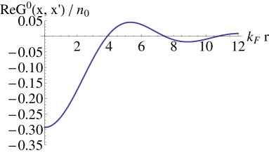
(a)

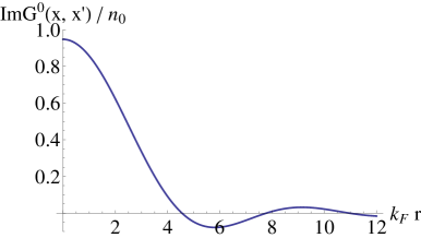
(b)

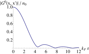
(c)

Figure 2: Real part, imaginary part and modulus of $G^{0}(x,x^{\prime})$ normalized to the density $n_{0}$ for $\Delta_{t}=0.5$ .

The above findings are borne out by the results shown in Figs. 1,  2 and  3, where one sees the behaviour of the modulus of $G^{0}(x,x^{\prime})$ versus $k_{F}r$ for a few values of $\Delta_{t}$. Also shown in Figs. 2 and  3 are the real and imaginary parts of $G^{0}(x,x^{\prime})$ for two finite values of $\Delta_{t}$. As is well-known in $({\vec{k}},\omega)$ space, these are connected through a dispersion relation.

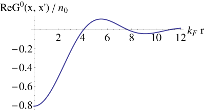
(a)

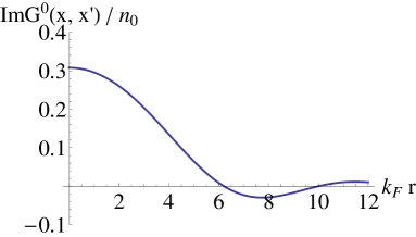
(b)

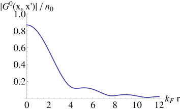
(c)

Figure 3: Same as in Fig. 2, but for $\Delta_{t}=2$ .

Importantly for $\Delta_{t}=0$ the hole propagator becomes purely imaginary and displays an oscillatory behaviour versus $k_{F}r$. This accounts for the zeros in its modulus shown in Fig. 1. From the point of view of the Heisenberg principle $\Delta_{t}=0$ corresponds to the maximum energy (in fact momentum) uncertainty for the propagating particle. Thus the wave function of the latter corresponds to a large superposition of plane waves yielding the striking zeros seen in Fig. 1. For $\Delta_{t}$ small, but not vanishing (Fig. 2), the propagator starts to develop a real part. This also oscillates, but its zeros differ from those of the imaginary part. Accordingly, now the particle can be found everywhere in space, but of course with a small probability when in the vicinity of the zeros appearing in Fig. 1. As $\Delta_{t}$ grows (Fig. 3) so does the real part of $G^{0}(x,x^{\prime})$ and the behaviour of the modulus of the propagator becomes smoother and smoother, until for $\Delta_{t}$ very large it becomes constant: indeed now, in accord with the Heisenberg principle, the wave function of the particle becomes a plane wave.

III The Coulomb sum rule

To pave the way to the more general treatment of the two-particle propagator (of which the density-density correlation function is a particular branch) to be discussed in the next section, we once more derive the well-known Coulomb sum rule, although this time through a somewhat different technique, namely an integration in coordinate space. For this purpose we recall (see  FW ) that, using standard quantum mechanics, the CSR can be cast in the form

$$S(\vec{q})=<\Psi_{0}|\tilde{\rho}^{\dagger}(-\vec{q})\tilde{\rho}(-\vec{q})|\Psi_{0}>\ ,$$ (8)

where $|\Psi_{0}>$ is the system’s ground state and $\tilde{\rho}(-\vec{q})$ is the density deviation operator defined as

$$\tilde{\rho}(-\vec{q})=\hat{\rho}(-\vec{q})-<\Psi_{0}|\hat{\rho}(-\vec{q})|\Psi_{0}>~{}.$$ (9)

It is then a straightforward matter to obtain from Eq. (8) the formula

$$S(\vec{q})=Z+\int d\vec{x}d\vec{y}e^{-i\vec{q}\cdot(\vec{x}-\vec{y})}<\Psi_{0}|\hat{\Psi}_{\alpha}^{\dagger}(\vec{x})\hat{\Psi}_{\beta}^{\dagger}(\vec{y})\hat{\Psi}_{\beta}(\vec{y})\hat{\Psi}_{\alpha}(\vec{x})|\Psi_{0}>-\rho_{0}^{2}V\delta(\vec{q})$$ (10)

which expresses the CSR in terms of the fermion fields in the Schroedinger picture (spin indices have been reintroduced) always sticking to the model of a homogeneous system enclosed in a large volume $V$ having $Z=A/2$ charges, with $A$ being the total number of spin $1/2$ particles. In the second term on the right-hand side of Eq. (10) one recognizes the equal-time two-particle propagator. This can be expressed in terms of the correlations among the particles in the system and indeed, in our simple case, it reads

$$<\Psi_{0}|\hat{\Psi}_{\alpha}^{\dagger}(\vec{x})\hat{\Psi}_{\beta}^{\dagger}(\vec{y})\hat{\Psi}_{\beta}(\vec{y})\hat{\Psi}_{\alpha}(\vec{x})|\Psi_{0}>=n_{0}^{2}\bigg{[}1-\frac{1}{2}\bigg{(}\frac{3j_{1}(k_{F}r)}{k_{F}r}\bigg{)}^{2}\bigg{]}=n_{0}^{2}\Big{[}1-\frac{1}{2}g^{2}(k_{F}r)\Big{]}$$ (11)

with $r\equiv|\vec{x}-\vec{y}|$. The function $\frac{1}{2}g^{2}(k_{F}r)$ is usually referred to as the Pauli pair correlation function. In the above the direct and exchange contributions clearly appear. Moreover it should be kept in mind that basic in deriving Eq. (11) have been the $\theta$-functions entering in $G^{0}({\vec{k}},\omega)$. Our aim here is to show that even small variations of Eq. (11) at short distances (and hence of the $\theta$-functions in momentum space) can produce quite dramatic changes in the CSR (see Sec. V).

We proceed by inserting Eq. (11) into Eq. (10), getting for the latter

$$S(\vec{q}) = Z+n_{0}^{2}V\delta(\vec{q})-n_{0}^{2}V\int d\vec{r}e^{-i\vec{q}\cdot\vec{r}}\frac{1}{2}\bigg{(}\frac{3j_{1}(k_{F}r)}{k_{F}r}\bigg{)}^{2}-n_{0}^{2}V\delta(\vec{q})$$ (12)

$$= Z\bigg{[}1-\frac{6}{\pi}\int_{0}^{\infty}dzj_{1}^{2}(z)j_{0}\bigg{(}\frac{q}{k_{F}}z\bigg{)}\bigg{]}\ ,$$

where the elementary angular integrations have been performed and the term arising from the direct piece of Eq. (11) is seen to drop out.

The integral in Eq. (12) can be computed in the complex $z$-plane using standard techniques (see Appendix B for details), yielding for the Coulomb sum rule the familiar non-relativistic expression FW

$$S(\vec{q}) = \begin{cases}Z\Big{(}\frac{3}{4}\frac{q}{k_{F}}-\frac{1}{2}\Big{(}\frac{q}{2k_{F}}\Big{)}^{3}\Big{)}&\text{if $q<2k_{F}$}\\ Z&\text{if $q\geq 2k_{F}$}~{}.\end{cases}$$ (13)

In connection with the above derivation which is valid for a perfect Fermi gas, it should be pointed out that the result in Eq. (13) stems from the exact cancellation of two contributions, as shown in Appendix B. We shall then prove in Section V that, as anticipated above, even a minor modification induced by interactions among the system’s constituents of the $\theta$-functions entering in $G^{0}({\vec{k}},\omega)$ is sufficient to disrupt the cancellation in Eq. (42): hence such a modification induces a sizable change of the CSR for large $q$. Since, as will be shown in Sec. V, modifying the $\theta$-function around the value $k=k_{F}$ actually corresponds to modifying the pair distribution in Eq. (11) for small distances, this outcome is what one should expect and it offers a nice example of how the Fourier transform works.

IV The density-density correlation function

In this section we analytically compute and explore in space-time the branch of the two-particle propagator usually referred to as the density-density correlation function or polarization propagator $\Pi(x,y)$. The expression for the latter is again well-known in energy-momentum space for a non-interacting system, as is the fact that its imaginary part provides the inelastic scattering cross section for many types of probes of a many-body system.

The definition of $\Pi(x,0)$ is the following

$$\Pi(x,0)=-i<\Psi_{0}|T(\tilde{\rho}_{H}(x)\tilde{\rho}_{H}(0))|\Psi_{0}>\ ,$$ (14)

where the density deviation operators are in the Heisenberg picture, unlike the case of the CSR where they were taken in the Schroedinger picture, i.e., where no T-product was introduced. To explore this point further we recast Eq. (14) in the form

$$\Pi(x,0)=-i \{ <\Psi_{0}|T(\hat{\Psi}_{\alpha}^{\dagger}(x)\hat{\Psi}_{\alpha}(x)\hat{\Psi}_{\beta}^{\dagger}(0)\hat{\Psi}_{\beta}(0))|\Psi_{0}>$$ (15)

$$- <\Psi_{0}|\hat{\Psi}_{\alpha}^{\dagger}(x)\hat{\Psi}_{\alpha}(x)|\Psi_{0}><\Psi_{0}|\hat{\Psi}_{\beta}^{\dagger}(0)\hat{\Psi}_{\beta}(0)|\Psi_{0}>\}~{}.$$

A comparison with Eq. (10) then shows that what enters in the CSR is just the above expression, however with the T-product replaced by its equal-time specification and it is precisely this quantity which is directly connected with the pair distribution function. As we have seen (and as we will discuss in more detail later) the latter crucially affects the CSR, namely, the frequency integral of the response.

The response, however, is not directly expressible in terms of the pair distribution correlation function, but rather the momentum distribution of the system’s constituents (in our case a $\theta$-function) enters into its definition. It thus appears that the $\theta$-function should be viewed as the fundamental ingredient of both the system’s response and of the CSR. Indeed in Sec. V we shall illustrate how the pair distribution function (and hence the CSR) is determined by the momentum distribution.

To proceed further, observe that with a straightforward application of Wick’s theorem to Eq. (15) one obtains for the non-interacting Fermi system

$$\Pi^{0}(x,0)=-2iG^{0}(x,0)G^{0}(x,0)~{}.$$ (16)

To compute this we start from the Fourier transform of its well-known expression in energy-momentum space

$$\Pi^{0}(q) = \big{(}-2i\big{)}\int\frac{d^{4}k}{(2\pi)^{4}}G^{0}(k)G^{0}(k+q)$$

$$= 2\int\frac{d\vec{k}}{(2\pi)^{3}}\theta(|\vec{k}+\vec{q}|-k_{F})\theta(k_{F}-k)\bigg{[}\frac{1}{q_{0}+\omega_{\vec{k}}-\omega_{\vec{q}+\vec{k}}+i\eta}-\frac{1}{q_{0}-\omega_{\vec{k}}+\omega_{\vec{q}+\vec{k}}-i\eta}\bigg{]}\ ,$$

where the integration on $k^{0}$ has been performed in the complex plane. Next we take the inverse Fourier transform of Eq. (IV)

$$\Pi^{0}(x,0)=\int\frac{d^{4}q}{(2\pi)^{4}}e^{iq\cdot x}\Pi^{0}(q)$$ (18)

and carry out the $q_{0}$-integration in the complex plane: this again distinguishes between forward and backward time propagation, corresponding to the two terms generated by the T-product. Both of these diverge for $t_{x}=0$ in accord with what was previously found for the one-fermion propagator. Here we recall that only the particle piece of the latter was seen to diverge at equal times. We shall return on this point later on.

Furthermore, the second term of $\Pi^{0}(x,0)$, associated with $q_{0}<0$, describes, the system’s response in the time-like domain. One obtains

$$\Pi^{0}(x,0) = -2i\int\frac{d\vec{q}}{(2\pi)^{3}}e^{i\vec{q}\cdot\vec{x}}\int\frac{d\vec{k}}{(2\pi)^{3}}\theta(k_{F}-k)\theta(|\vec{k}+\vec{q}|-k_{F})$$ (19)

$$\times\bigg{\{}e^{-i\big{(}\frac{q^{2}}{2m}+\frac{1}{m}\vec{q}\cdot\vec{k}\big{)}t_{x}}\theta(t_{x})+e^{i\big{(}\frac{q^{2}}{2m}+\frac{1}{m}\vec{q}\cdot\vec{k}\big{)}t_{x}}\theta(-t_{x})\bigg{\}}~{}.$$

After some algebra (see Appendix C for details) the above expression can be reduced to a single integral (we focus on the first piece, since the second one is immediately derived when the first is known):

$$\Pi^{0}(x,0)\theta(t_{x})=-\frac{9in_{0}^{2}}{4\Delta_{t}k_{F}r}\bigg{\{}\int_{2}^{\infty}dse^{-i\Delta_{t}s^{2}}\sin(sk_{F}r)j_{1}(2\Delta_{t}s)$$

$$+\int_{1}^{2}dse^{-i\Delta_{t}s^{2}}\sin(sk_{F}r)j_{1}(2\Delta_{t}s(s-1))(s-1)^{2}$$

$$+\frac{1}{2\Delta_{t}}\int_{1}^{2}ds\sin(sk_{F}r)\bigg{[}e^{-i\Delta_{t}s^{2}}\cos(2\Delta_{t}s(s-1))-e^{-2i\Delta_{t}s^{2}}\bigg{(}\frac{1}{s}\cos\Big{(}\Delta_{t}s(s-2)\Big{)}$$

$$+\frac{1}{2\Delta_{t}s^{2}}\sin\Big{(}\Delta_{t}s(s-2)\Big{)}\bigg{)}\bigg{]}+\frac{1}{2\Delta_{t}}\int_{0}^{1}ds\sin(sk_{F}r)e^{-2i\Delta_{t}s}\sin(2\Delta_{t}s^{2})\frac{1}{s}\bigg{(}\frac{1}{2\Delta_{t}s}+i\bigg{)}$$

$$+\frac{\cos(2k_{F}r)-1}{4\Delta_{t}k_{F}r}\bigg{\}}~{},$$ (20)

where $r\equiv|\vec{x}|$ and $s=q/k_{F}$. As previously anticipated, in the limit of vanishing $\Delta_{t}$ the above becomes purely imaginary and diverges.

To show that this divergence is as severe as the one encountered for the one-particle propagator (see Eq. (3)) we consider the first term inside the curly brackets. Here we are allowed to replace the spherical Bessel function with his leading term in the small argument expansion getting

$$\frac{2\Delta_{t}}{3}\int_{2}^{\infty}dse^{-i\Delta_{t}s^{2}}\sin(sk_{F}r)\simeq\frac{1}{2}\sqrt{\frac{\pi}{\Delta_{t}i^{3}}}\frac{k_{F}r}{3}e^{i\frac{(k_{F}r)^{2}}{4\Delta_{t}}}~{}.$$ (21)

Hence our statement follows.

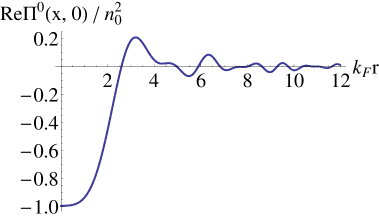
(a)

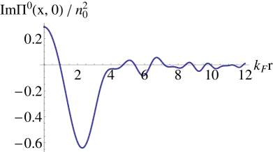
(b)

(c)

Figure 4: Real part (a), imaginary part (b) and modulus (c) of $\Pi^{0}(x,0)$ divided by $n_{0}^{2}$ and plotted versus $k_{F}r$ for $\Delta_{t}=0.8$ and three values of $k_{F}$: 1.2, 1.36 and 1.5 fm^-1. Note that the same curve is obtained for any value of $k_{F}$.

In Figs. 4 - 6 we display the modulus of $\Pi^{0}(x,0)$ together with its real and imaginary parts for a few values of $\Delta_{t}$. We observe that for small $\Delta_{t}$ a diffraction pattern emerges as in the case of the single-particle propagator: indeed, from the Heisenberg principle, here the energy is considerably spread out and, as a consequence, a wave packet can be set up which vanishes at fixed positions selected by the medium. As $\Delta_{t}$ increases this pattern is washed out until for very large $\Delta_{t}$ it turns into an almost uniform behaviour. From the formal point of view this evolution reflects the fact that for small time differences the particle-hole propagator is essentially imaginary, just as happened for the one-hole propagator. This imaginary part oscillates with the distance and hence the diffraction pattern follows. However, as the time difference increases a real part develops, also with an oscillatory behaviour, but with zeros displaced with respect to those of the imaginary part. Hence the zeros of the diffraction pattern are lifted up until at large $\Delta_{t}$ the modulus of $\Pi^{0}(x,0)$ becomes uniform in space.

A further important feature of $\Pi^{0}(x,0)$ relates to its rapid decrease occurring in the range $0<k_{F}r\lesssim 4$: we have numerically checked that in this domain all the terms in Eq. (IV) contribute by roughly the same amount whereas for larger $k_{F}r$ the integrals with the variable running in the intervals $(0,1)$ and $(1,2)$, where the Pauli correlations are operative, essentially drop out. We thus conclude that are these correlations which damp the propagation of a density disturbance in the system.

We turn now to the evaluation of the remaining integrals with respect to the variable $q$ to complete our task of obtaining an analytic expression for $\Pi^{0}(x,0)$. For this purpose we introduce the dimensionless quantities

$$z=\frac{k_{F}r}{2\sqrt{\Delta_{t}}}\mbox{ and }\rho=\sqrt{\Delta_{t}}$$ (22)

and the function

$$g(a,b,c)=\int_{a}^{b}dy\frac{e^{iy^{2}}}{y+c}~{}.$$ (23)

The latter can in fact be expressed in terms of the Meijer-$G$ functions Abr , although the resulting formulas are quite cumbersome and hence we prefer to use directly the definition expressed by Eq. (23). Even so the remaining $q$-integrations are, unfortunately, given by expressions which are far from simple; we report these in Appendix C for completeness.

To pave the way to Appendix C here we simply rewrite Eq. (IV) in terms of the variables in Eq. (22). It becomes

$$\Pi^{0}_{a}(x,x^{\prime}) = -in_{0}^{2}\frac{9}{8z}\frac{1}{\rho^{3}}\int_{2}^{\infty}dse^{-i\rho^{2}s^{2}}\sin(2\rho zs)j_{1}(2\rho^{2}s)$$ (24)

$$\simeq -in_{0}^{2}\frac{3}{2}\int_{2}^{\infty}dse^{-i\rho^{2}s^{2}}s^{2}\,\,\,\mbox{\rm for }\rho\to 0$$

$$\Pi^{0}_{b}(x,x^{\prime}) = -in_{0}^{2}\frac{9}{8z}\frac{1}{\rho^{3}}\int_{1}^{2}dse^{-i\rho^{2}s^{2}}\sin(2\rho zs)j_{1}(2\rho^{2}s(s-1))(s-1)^{2}$$ (25)

$$\simeq -in_{0}^{2}\frac{49}{40}\,\,\,\mbox{\rm for }\rho\to 0$$

$$\Pi^{0}_{c}(x,x^{\prime}) = -in_{0}^{2}\frac{9}{16z}\frac{1}{\rho^{5}}\int_{1}^{2}ds\sin(2\rho sz)\left\{e^{-i\rho^{2}s^{2}}\cos(2\rho s(1-s))-e^{-2i\rho^{2}s^{2}}\right.$$ (26)

$$\times \left.\left[\cos(\rho^{2}s(s-2))+\frac{1}{2\rho^{2}s}\sin(\rho^{2}s(s-2))\right]\right\}$$

$$\simeq -in_{0}^{2}\frac{21}{16}\frac{1}{\rho^{4}}\,\,\,\mbox{\rm for }\rho\to 0$$

$$\Pi^{0}_{d}(x,x^{\prime}) = -in_{0}^{2}\frac{9}{16z}\frac{1}{\rho^{5}}\left\{\frac{\cos(4\rho z)-1}{8z\rho^{3}}k_{F}^{3}+\int_{0}^{1}ds\sin(2\rho sz)e^{-2i\rho^{2}s}\sin(2\rho^{2}s^{2})\frac{1}{s}\left(\frac{1}{2s\rho^{2}}+i\right)\right\}$$ (27)

$$\simeq in_{0}^{2}\frac{9}{8}\frac{z}{\rho^{4}}\,\,\,\mbox{\rm for }\rho\to 0$$

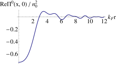
(a)

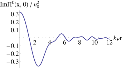
(b)

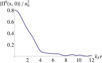
(c)

Figure 5: As for Fig. 4, but now with $\Delta_{t}=1$ .

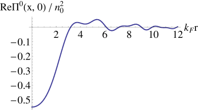
(a)

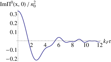
(b)

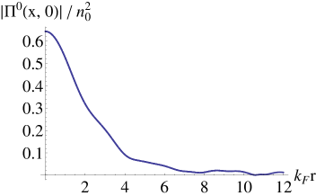
(c)

Figure 6: As for Fig. 5, but now with $\Delta_{t}=1.2$ .

Concerning this all important issue, referred to as second kind scaling, much light on it is shed by the analysis of $\Pi^{0}(x,0)$ in space-time coordinates. Here one realizes that just as $G^{0}(x,x^{\prime})$ turned out to be proportional to $n_{0}$ (see Eq. (II)), $\Pi^{0}(x,0)$ is proportional to $n_{0}^{2}$ as expected. Then, when these density factors are divided out in both propagators one finds that $G^{0}(x,x^{\prime})$ and $\Pi^{0}(x,0)$ scale at any $\Delta_{t}$ providing that the space-time coordinates are in turn rescaled in terms of the Fermi momentum and frequency. This is clearly illustrated in Figs. 4, 5 and 6 where the spatial behaviour of the $\Pi^{0}(x,0)$ associated with three different values of $k_{F}$ is displayed as a function of $k_{F}r$. The curves are seen to coincide at $\Delta_{t}=0.8$, $1$ and $1.2$, in accord with Eq. (IV), which transparently exhibits the $k_{F}$-scaling property.

The above results concerning $\Pi^{0}(x,0)$ should, however, be viewed with some care. This is because the search for scaling in $k_{F}$ at vanishing $\Delta_{t}$ is impossible owing to the divergence discussed above which signals that the theory is ill-defined. Actually all of the terms in Eqs. (IV) diverge at $\Delta_{t}=0$, with the exception of the second one.

V The impact of a more realistic momentum distribution

Here we explore the impact of interactions among the constituent fermions on the pair correlation function and the CSR. This we do in a schematic frame that should, however, capture some of the relevant physics. We assume for the momentum distribution $n(k)$ the expression

$$n(k)=\theta(k_{F}-k)(1-\alpha\frac{k^{2}}{k_{F}^{2}})+\theta(k-k_{F})\beta_{1}e^{-\beta_{2}(\frac{k}{k_{F}}-1)}~{}.$$ (28)

The four parameters (indeed also $k_{F}$ should be viewed as such) entering in Eq. (28) must satisfy the normalization condition

$$\frac{k_{F}^{3}}{\pi^{2}}\bigg{[}\frac{1}{3}-\frac{\alpha}{5}+\frac{\beta_{1}}{\beta_{2}^{3}}(\beta_{2}^{2}+2\beta_{2}+2)\bigg{]}=n_{0}\ ,$$ (29)

where $n_{0}$ is the experimental constant density of the system. Notice that for $1-\alpha=\beta_{1}$ the Fermi system becomes superconductive (the Fermi surface disappears) whereas for $1-\alpha>\beta_{1}$ the discontinuity at the Fermi surface remains, as it should for a normal Fermi system according to the Luttinger Lutt theorem. This implies that both $\alpha$ and $\beta_{1}$ should be positive.

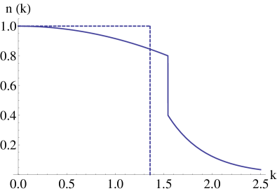
Figure 7: The momentum distribution of an interacting Fermi system as given by formula Eq. (28) of the text. The following values for the parameters have been chosen $k_{F}=1.54$ fm^-1, $\alpha=0.2$ , $\beta_{1}=0.4$ and $\beta_{2}=4$ . The non interacting case (dotted line) corresponds to $k_{F}=1.36$ fm^-1 .

We now choose as an example nuclear matter (in this case the left-hand side of Eq. (29) should be multiplied by $2$ to account for the isospin degeneracy) where one has $n_{0}=0.17$ fm^-3. We then display in Fig. 7 the $n(k)$ for nuclear matter for a specific choice for the four parameters, chosen to fulfill both Eq. (29) and the above-mentioned constraint. The tail at large momenta is evident and one finds that the new Fermi momentum turns out to be $k_{F}=1.54$ fm^-1, namely larger that the one associated with the non-interacting case.

The pair correlation function for the momentum distribution in Eq. (28) is then easily computed and reads

$$<\Psi_{0}|\hat{\Psi}_{\alpha}^{\dagger}(\vec{x})\hat{\Psi}_{\beta}^{\dagger}(\vec{0})\hat{\Psi}_{\beta}(\vec{0})\hat{\Psi}_{\alpha}(\vec{x})|\Psi_{0}>=n_{0}^{2}\Big{\{}1-\frac{1}{2}g^{2}(r)\Big{\}}$$

$$=n_{0}^{2}\Bigg{\{}1-\frac{1}{2}\bigg{\{}\frac{3}{k_{F}r}\bigg{[}j_{1}(k_{F}r)-\frac{\alpha}{(k_{F}r)^{4}}\Big{(}3((k_{F}r)^{2}-2)\sin(k_{F}r)$$

$$-k_{F}r((k_{F}r)^{2}-6)\cos(k_{F}r)\Big{)}+\beta_{1}\Big{(}\frac{k_{F}r}{(k_{F}r)^{2}+\beta_{2}^{2}}\Big{)}^{2}$$ (30)

$$\times\Big{(}\sin(k_{F}r)\Big{(}\beta_{2}+\frac{\beta_{2}^{2}+\beta_{2}^{3}}{(k_{F}r)^{2}}-1\Big{)}+\cos(k_{F}r)\Big{(}k_{F}r+\frac{2\beta_{2}+\beta_{2}^{2}}{k_{F}r}\Big{)}\Big{)}\bigg{]}\bigg{\}}^{2}\Bigg{\}}~{}.$$

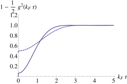
Figure 8: The pair correlation function $1-\frac{1}{2}g^{2}(k_{F}r)$ for a free (dotted line) and for an interacting (continuos line) Fermi gas as given by our model (formula  (V) of the text). The values of parameters are the same as in Fig. 7 . Note that the two curves refer to different $k_{F}$ .

Using the same values of the parameters as for the momentum distribution shown in Fig. 7, this pair correlation function is displayed in Fig. 8 where it is compared with that of the pure Fermi gas from Eq. (11). What clearly appears in the figure is the marked difference between the two correlations functions at short distances, while they practically coincide at large distances: this behaviour nicely illustrates the role of the short-range correlations.

Finally, we compute the CSR using Eq. (V). Although also in this case the calculation can be analytically performed using complex coordinates, as was previously done in the non-interacting situation, the resulting expression turns out to be very cumbersome; hence we resort to the numerical evaluation of the formula

$$S(\vec{q})=Z-n_{0}^{2}\frac{1}{2}\int d\vec{r}e^{-i\vec{q}\cdot\vec{r}}g^{2}(r)\ ,$$ (31)

the function $g(r)$ being defined in Eq. (V).

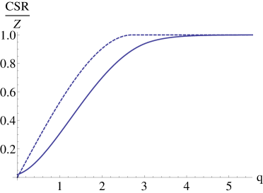
Figure 9: The Coulomb sum rule (see Eq. (31) of the text) for a free Fermi gas (dotted line) and for a correlated one according to our model (continuous line). The parameters are the same as in Fig. 7 and Fig. 8 .

The outcome is shown in Fig. 9 where it is clearly seen that results from Eq. (31) coincide with those from Eq. (13) at large $q$ (say $q>4$ fm^-1), as they should, since in this domain of momenta the associated wavelengths are so small that the system appears to the probe as a collection of uncorrelated fermions. On the other hand for, say, $2.5<q<4$ fm^-1 the two sum rules differ substantially due to the action of the correlations among the fermions. Finally, for smaller $q$ this difference tends to disappear as both sum rules should go to zero when $q$ vanishes. Noteworthy is that the sum rule arising from Eq. (31) reaches the asymptotic value 1 from below.

VI Conclusions

In this work we have deduced expressions for the one- and two-particle propagators as functions of space-time coordinates, focusing on the hole propagator and the density-density correlator. To our knowledge these expressions were not previously available in the literature. We find that both propagators have infinities at equal time, a problem that is being addressed in other work. Next we have explored the asymptotic space-time behaviour of both Green functions and have found a transition from a diffractive regime to a uniform one as the time difference between the fields (for the one-particle propagator) or between the densities (for the two-particle propagator) grows. From the formal point of view this relates to the fact that both propagators for zero time difference are purely imaginary, but then the real parts start to develop as the time difference grows. Concerning the dependence upon $k_{F}$, our analysis shows that both $G^{0}$ and $\Pi^{0}$ scale once appropriate measures for space and time are chosen. This outcome goes in parallel with the situation in frequency-momentum space. However the divergence affecting $\Pi^{0}$ at $\Delta_{t}=0$ prevents the analysis of second-kind scaling for this propagator at vanishing $\Delta_{t}$.

We have found that the key ingredient contained in the propagators is the momentum distribution $n(k)$. For example the Coulomb sum rule can be directly expressed in terms of the pair correlation function, which can, of course, be obtained once $n(k)$ is known. We have explored the consequences arising from a modification around the Fermi surface of $n(k)$ away from the pure Fermi gas result, finding that this induces striking effects in the pair correlation function at short distances. This in turn leads to major differences in the Coulomb sum rule for momenta between about $2.5$ and $4$ fm^-1 for the model used in the present study, suggesting that it would be interesting to explore the responses of our infinite Fermi system to external probes, employing in the calculation of the polarization propagator our modified momentum distribution function given in Eq. (28). This, of course, is meant to account for the correlations (possibly of short range) among the fermions.

A further issue, in some sense complementary to the above one, deserves consideration. It relates to the passage from an infinite to a finite system, the latter obviously of concern for nuclear physics. As a first approximation this transition can be accomplished by accounting for the modification of the density of the single-particle states induced by the presence of the system’s surface according to the prescription given by Feshbach Fesh . In a preliminary investigation we have done so and found, as expected, that the impact of the surface in coordinate space on the system’s response is only felt at low momenta. More specifically, the confinement on the one hand entails oscillations of the system’s density in coordinate space, on the other enlarges the momentum distribution $n(k)$ to momenta greater than those of the corresponding infinite system with equal density. At the same time it digs a hole at low $k$ in the momentum distribution. Thus confinement (in leading order) and short-range correlations appear to work in the same direction at large momenta. The disentangling of the interplay between the two effects is a problem we intend to address in forthcoming work. We will also explore in depth how the scaling of first kind is reflected in the space-time coordinates.

Finally, since much of the physics we are addressing here occurs at large momenta, it is imperative to extend the present treatment to the relativistic context, with the goal of providing a comparison between the results one would obtain using the present approach and those already obtained in other approaches to electroweak superscaling. For instance, it will be of interest to answer the question: How will scaling in $k_{F}$ of the imaginary part of the polarization propagator occurring for all values of space-time coordinates in the non-interacting, homogeneous case be affected (and eventually disrupted) by confinement and short-range correlations in both the non-relativistic and relativistic context?

Appendix A

In this appendix we analyze the behaviour of the propagator $G^{0}(x,x^{\prime})$ for very small $\Delta_{t}$. For this purpose we use the well-known asymptotic expansion of the error function

$$erf(z)=1-\frac{1}{\sqrt{\pi}z}e^{-z^{2}}\Bigg{[}1+\sum_{m=1}^{\infty}(-1)^{m}\frac{(2m-1)!!}{(2z^{2})^{m}}\Bigg{]}~{}.$$ (32)

Then from the above, after some algebra, in leading order of $\Delta_{t}$ one obtains for the third term on the right-hand side of the propagator in Eq. (II)

$$\frac{1}{2}\frac{k_{F}|{\vec{x}}-{\vec{x}^{\prime}}|}{2\Delta_{t}}\bigg{(}\frac{e^{ik_{F}|{\vec{x}}-{\vec{x}^{\prime}}|}}{k_{F}|{\vec{x}}-{\vec{x}^{\prime}}|+2\Delta_{t}}-\frac{e^{-ik_{F}|{\vec{x}}-{\vec{x}^{\prime}}|}}{k_{F}|{\vec{x}}-{\vec{x}^{\prime}}|-2\Delta_{t}}\bigg{)}$$

$$=-\frac{1}{2i\Delta_{t}}\sin(k_{F}|{\vec{x}}-{\vec{x}^{\prime}}|)-\frac{\cos(k_{F}|{\vec{x}}-{\vec{x}^{\prime}}|)}{k_{F}|{\vec{x}}-{\vec{x}^{\prime}}|}$$ (33)

which exactly cancels the second term of the right-hand side; hence Eq. (7) follows.

Appendix B

Here we compute the integral in Eq. (12) working in the complex $z$-plane. Setting ${\overline{q}}=q/k_{F}$, we have

$$I = \int_{0}^{\infty}dzj_{1}^{2}(z)j_{0}(\overline{q}z)=\frac{1}{2}\int_{-\infty}^{\infty}dz\bigg{(}\frac{\sin z}{z^{2}}-\frac{\cos z}{z}\bigg{)}^{2}\frac{\sin(\overline{q}z)}{\overline{q}z}$$ (34)

$$= \frac{1}{2\overline{q}}\int_{-\infty}^{\infty}\frac{dz}{z^{5}}(\sin z-z\cos z)^{2}\sin(\overline{q}z)~{}.$$

The integrand, which behaves as $\sim z^{2}$ for $z\rightarrow 0$, is a regular analytic function; hence the integration path along the real axis can be deformed by inserting a very small semicircle going around the origin from below. This we indicate with the symbol $\landdownint$. Closing the integration path along a large semicircle in the $Im\;z>0$ region, we thus get

$$I=\frac{i}{8\overline{q}}\landdownint_{-\infty}^{\infty}\frac{dz}{z^{5}} \Big{\{} (1-iz)^{2}e^{i(2+\overline{q})z}-(1-iz)^{2}e^{i(2-\overline{q})z}+(1+iz)^{2}e^{i(\overline{q}-2)z}$$ (35)

$$-(1+iz)^{2}e^{-i(\overline{q}+2)z}-2(1+z^{2})e^{i\overline{q}z}+2(1+z^{2})e^{-i\overline{q}z}\Big{\}}\ ,$$

where the fourth and the sixth term on the right-hand side do not contribute because for these the integration path has to be closed in the $Im\;z<0$ domain where no singularities exist. It is then convenient to split Eq. (35) into two pieces according to

$$I=I_{1}+I_{2}$$ (36)

with

$$I_{1}=\frac{i}{8\overline{q}}\landdownint_{-\infty}^{\infty}\frac{dz}{z^{5}}\Big{[}(1-iz)^{2}e^{i(\overline{q}+2)z}-2(1+z^{2})e^{i\overline{q}z}\Big{]}$$ (37)

and

$$I_{2}=\frac{i}{8\overline{q}}\begin{cases}\landdownint_{-\infty}^{\infty}\frac{dz}{z^{5}}(1+iz)^{2}e^{i(\overline{q}-2)z}&\text{if $\overline{q}>2$ }\\ -\landdownint_{-\infty}^{\infty}\frac{dz}{z^{5}}(1-iz)^{2}e^{i(2-\overline{q})z}&\text{if $\overline{q}<2$}~{}.\end{cases}$$ (38)

The straightforward, while somewhat tedious, computation of the residues then yields

$$I_{1}=-\frac{\pi}{8\overline{q}}\Big{\{}\frac{1}{4!}(\overline{q}+2)^{4}-\frac{2}{3!}(\overline{q}+2)^{3}+\frac{1}{2}(\overline{q}+2)^{2}-\frac{2}{4!}{\overline{q}}^{4}+{\overline{q}}^{2}\Big{\}}~{},$$ (39)

$$I_{2}=-\frac{\pi}{8\overline{q}}\Big{\{}\frac{1}{4!}(\overline{q}-2)^{4}+\frac{2}{3!}(\overline{q}-2)^{3}+\frac{1}{2}(\overline{q}-2)^{2}\Big{\}} \overline{q}>2$$ if (40)

and

$$I_{2}=+\frac{\pi}{8\overline{q}}\Big{\{}\frac{1}{4!}(\overline{q}-2)^{4}+\frac{2}{3!}(\overline{q}-2)^{3}+\frac{1}{2}(\overline{q}-2)^{2}\Big{\}} \text{if $\overline{q}<2$ }~{}.$$ (41)

As a result of the cancellation occurring between Eqs. (39) and (40) one thus finds

$$I=I_{1}+I_{2}=0 \overline{q}>2$$ if (42)

and

$$I=I_{1}+I_{2}=\frac{\pi}{8}\Big{(}\frac{4}{3}-\overline{q}+\frac{1}{12}{\overline{q}}^{3}\Big{)} \text{if $\overline{q}<2$ }~{}.$$ (43)

Appendix C

In this appendix we perform the integrals in Eq. (19). We focus on the first piece, since the second one is immediately derived once the first is known. For these pieces three angular integrations are trivial whereas the fourth should be approached with care owing to the presence of the $\theta$-function, leading naturally to the splitting of the integral over the modulus of the vector $\vec{q}$ into three pieces:

$$\Pi^{0}(x,0)\theta(t_{x})=-\frac{4i}{r}\int_{0}^{k_{F}}\frac{dk}{(2\pi)^{2}}k^{2}$$

$$\times\bigg{\{}\int_{2k_{F}}^{\infty}\frac{dq}{(2\pi)^{2}}qe^{-i\frac{q^{2}}{2m}t_{x}}\sin(qr)\int_{-1}^{1}d\cos\theta e^{-i\frac{qk\cos\theta}{m}t_{x}}$$

$$+\int_{k_{F}}^{2k_{F}}\frac{dq}{(2\pi)^{2}}qe^{-i\frac{q^{2}}{2m}t_{x}}\sin(qr)\int_{max\big{[}\frac{k_{F}^{2}-q^{2}-k^{2}}{2qk},-1\big{]}}^{1}d\cos\theta e^{-i\frac{qk\cos\theta}{m}t_{x}}$$ (44)

$$+\int_{0}^{k_{F}}\frac{dq}{(2\pi)^{2}}qe^{-i\frac{q^{2}}{2m}t_{x}}\sin(qr)\int_{\frac{k_{F}^{2}-q^{2}-k^{2}}{2qk}}^{1}d\cos\theta e^{-i\frac{qk\cos\theta}{m}t_{x}}\theta\bigg{(}1-\frac{k_{F}^{2}-q^{2}-k^{2}}{2qk}\bigg{)}\bigg{\}}~{}.$$

The remaining angular integration is trivial and the integral over the modulus of the vector $\vec{k}$, while somewhat cumbersome, can be performed. Introducing for convenience a time variable with the dimensions of a length squared, $\tau=t_{x}/m$, one arrives at the expression

$$\Pi^{0}(x,0)\theta(t_{x})=-\frac{i}{2\pi^{4}\tau r}\bigg{\{}k_{F}^{2}\int_{2k_{F}}^{\infty}dqe^{-i\frac{\tau}{2}q^{2}}\sin(qr)j_{1}(\tau qk_{F})$$

$$+\int_{k_{F}}^{2k_{F}}dqe^{-i\frac{\tau}{2}q^{2}}\sin(qr)j_{1}(\tau q(q-k_{F}))(q-k_{F})^{2}$$

$$+\frac{1}{\tau}\int_{k_{F}}^{2k_{F}}dq\sin(qr)\bigg{[}e^{-i\frac{\tau}{2}q^{2}}\cos(\tau q(k_{F}-q))-e^{-i\tau q^{2}}\bigg{(}\frac{k_{F}}{q}\cos\Big{(}\tau\Big{(}\frac{q^{2}}{2}-qk_{F}\Big{)}\Big{)}$$

$$+\frac{1}{\tau q^{2}}\sin\Big{(}\tau\Big{(}\frac{q^{2}}{2}-qk_{F}\Big{)}\Big{)}\bigg{)}\bigg{]}+\frac{1}{\tau}\int_{0}^{k_{F}}dq\sin(qr)e^{-i\tau qk_{F}}\sin(\tau q^{2})\bigg{(}\frac{1}{\tau q^{2}}+i\frac{k_{F}}{q}\bigg{)}$$

$$+\frac{\cos(2k_{F}r)-1}{2\tau r}\bigg{\}}~{}.$$ (45)

Then, for the first term in Eq. (C), the $q$-integration between $2k_{F}$ and $\infty$ yields:

$$\Pi^{0}_{(1)}(x,0)\theta(t_{x})=-\frac{2}{(2\pi)^{4}}\frac{\theta(t_{x})}{\tau^{3}}\frac{1}{z}\Big{\{}\sqrt{2\pi}(1-i)e^{-2i\rho z}\cos(\rho^{2}+z^{2})$$ (46)

$$+(-2i\rho\sin(\rho+z)^{2}+e^{-i(\rho+z)^{2}}z)g^{*}(-\infty,+\infty,\rho+z)+e^{i(\rho-z)^{2}}(2\rho-z)g^{*}(-\infty,+\infty,\rho-z)\Big{\}}~{};$$

for the second term in Eq. (C) the $q$-integration between $k_{F}$ and $2k_{F}$ yields

$$\Pi^{0}_{(2a)}(x,0)\theta(t_{x})=-\frac{i}{(2\pi)^{4}}\frac{\theta(t_{x})}{\tau^{3}}\frac{1}{z}$$

$$\times\bigg{\{}-\frac{\sin(4\rho z)}{\rho}(1-e^{-i8\rho^{2}})+4\frac{e^{-i\rho^{2}}}{\rho}\sin(2\rho z)+\sqrt{\pi}\frac{1+i}{2}\Big{[}e^{-i(\rho-z)^{2}}erf\Big{(}\frac{1-i}{\sqrt{2}}(\rho+z)\Big{)}$$

$$-e^{i(\rho+z)^{2}}erf\Big{(}\frac{1-i}{\sqrt{2}}(\rho-z)\Big{)}-\big{(}e^{-i(\rho-z)^{2}}+e^{-i(\rho+z)^{2}}\big{)}erf\Big{(}\frac{1-i}{\sqrt{2}}z\Big{)}$$

$$-i\sqrt{3}\Big{(}erf\Big{(}\frac{1+i}{\sqrt{2}}\frac{1}{\sqrt{3}}(5\rho-z)\Big{)}-erf\Big{(}\frac{1+i}{\sqrt{2}}\frac{1}{\sqrt{3}}(2\rho-z)\Big{)}\Big{)}e^{\frac{i}{3}(\rho+z)^{2}}+(z\rightarrow-z)\Big{]}$$

$$-2\Big{[}e^{-i(\rho-z)^{2}}(\rho-z)g(z,\rho+z,\rho-z)-e^{i(\rho+z)^{2}}(\rho+z)g(-z,\rho-z,\rho+z)$$

$$+\Big{(}\frac{1}{\sqrt{3}}e^{\frac{i}{3}(\rho+z)^{2}}(\rho+z)g\Big{(}\frac{3\rho-z}{\sqrt{3}},\frac{5\rho-z}{\sqrt{3}},\frac{\rho+z}{\sqrt{3}}\Big{)}-(z\rightarrow-z)\Big{)}\Big{]}$$

$$-(1+i)\sqrt{\frac{\pi}{2}}\Big{[}\Big{(}e^{-i(\rho-z)^{2}}\Big{(}erf\Big{(}\frac{1-i}{\sqrt{2}}(\rho+z)\Big{)}-erf\Big{(}\frac{1-i}{\sqrt{2}}z\Big{)}\Big{)}-(z\rightarrow-z)$$

$$+\Big{(}\frac{1}{i}e^{\frac{i}{3}(\rho+z)^{2}}\Big{(}erf\Big{(}\frac{1+i}{\sqrt{2}}\frac{1}{\sqrt{3}}(5\rho-z)\Big{)}-erf\Big{(}\frac{1+i}{\sqrt{2}}\frac{1}{\sqrt{3}}(2\rho-z)\Big{)}\Big{)}-(z\rightarrow-z)\Big{)}$$

$$-\frac{2}{1+i}\sqrt{\frac{2}{\pi}}\rho\Big{(}\Big{(}e^{\frac{i}{3}(\rho+z)^{2}}g\Big{(}\frac{2\rho-z}{\sqrt{3}},\frac{5\rho-z}{\sqrt{3}},\frac{\rho+z}{\sqrt{3}}\Big{)}-(z\rightarrow-z)\Big{)}$$

$$+\Big{(}e^{-i(\rho-z)^{2}}g(\rho,2\rho,\rho-z)-(z\rightarrow-z)\Big{)}\Big{)}\Big{]}\Big{\}}$$ (47)

for the term embodying the $j_{1}$ and

$$\Pi^{0}_{(2b)}(x,0)\theta(t_{x})=-\frac{i}{(2\pi)^{4}}\frac{\theta(t_{x})}{\tau^{3}}\frac{1}{z}$$

$$\times\left\{e^{\frac{i}{3}(\rho+z)^{2}}\left(\frac{1}{\sqrt{3}}-2i\sqrt{3}\right)\sqrt{\frac{\pi}{2}}\frac{1-i}{2}\left[erf\left(\frac{1+i}{\sqrt{2}}\left(2\sqrt{3}\rho-\frac{\rho+z}{\sqrt{3}}\right)\right)\right.\right.$$

$$\left.-erf\left(\frac{1+i}{\sqrt{2}}\left(\sqrt{3}\rho-\frac{\rho+z}{\sqrt{3}}\right)\right)\right]-(z\rightarrow-z)$$

$$-e^{\frac{i}{3}(\rho+z)^{2}}\left[\rho\left(1-2i\right)-2iz\right]g^{*}\left(\sqrt{3}\rho-\frac{\rho+z}{\sqrt{3}},2\sqrt{3}\rho-\frac{\rho+z}{\sqrt{3}},\frac{z-\rho}{\sqrt{3}}\right)$$

$$+e^{\frac{i}{3}(\rho-z)^{2}}\left(\rho+2i\right)g^{*}\left(\sqrt{3}\rho-\frac{\rho-z}{\sqrt{3}},2\sqrt{3}\rho-\frac{\rho-z}{\sqrt{3}},\frac{\rho-z}{\sqrt{3}}\right)$$

$$-\left[e^{i(\rho+z)^{2}}\sqrt{\frac{\pi}{2}}\frac{1-i}{2}\left(erf\left(\frac{1+i}{\sqrt{2}}\left(\rho-z\right)\right)-erf\left(-\frac{1+i}{\sqrt{2}}z\right)\right)\right.$$

$$\left.-e^{-i(\rho+z)^{2}}\sqrt{\frac{\pi}{2}}\frac{1-i}{2}\left(erf\left(\frac{1+i}{\sqrt{2}}\left(\rho+z\right)\right)-erf\left(\frac{1+i}{\sqrt{2}}z\right)\right)\right]$$

$$+e^{i(\rho+z)^{2}}\left[\rho(1-2i)-2iz\right]g^{*}\left(2\rho+z,3\rho+z,-\rho-z\right)$$

$$+e^{-i(\rho-z)^{2}}\left[\sqrt{\frac{\pi}{2}}(1+i)\left(erf\left(\frac{1+i}{\sqrt{2}}(3\rho-z)\right)-erf\left(\frac{1+i}{\sqrt{2}}(2\rho-z)\right)\right)\right.$$

$$\left.+2i(\rho-z)g^{*}\left(2\rho-z,3\rho-z,z-\rho\right)-\rho g^{*}\left(2\rho-z,3\rho-z,-z+\rho\right)\right]$$

$$+e^{i\frac{z^{2}}{2}}\frac{\sqrt{\pi}}{2}\frac{1-i}{2}\left(erf\left(\frac{1+i}{\sqrt{2}}\left(\sqrt{2}\rho+\frac{z}{\sqrt{2}}\right)\right)-erf\left(\frac{1+i}{\sqrt{2}}\left(\sqrt{2}\rho-\frac{z}{\sqrt{2}}\right)\right)\right)$$

$$+\frac{1}{2\rho}\left[2e^{-i\rho(\rho-2z)}-e^{-4i\rho(2\rho-z)}-2e^{-i\rho(3\rho+2z)}+e^{-4i\rho(2\rho+z)}-2e^{-i\rho(\rho+2z)}+e^{-4i\rho(2\rho+z)}\right.$$

$$\left.\left.-2e^{-i(2z^{2}+5\rho^{2}-6\rho z)}+e^{-2i(z^{2}+5\rho^{2}-4\rho z)}\right]\right\}$$ (48)

for the other terms. Finally for the third term in Eq. (C) the $q$-integration between $0$ and $k_{F}$ yields:

$$\Pi^{0}_{(3)}(x,0)\theta(t_{x})=i\frac{2}{(2\pi)^{4}}\frac{\theta(t_{x})}{\tau^{3}}\frac{1}{z}\Bigg{\{}-\frac{\sin(2\rho z)}{i\rho}+\sqrt{\pi}\frac{1+i}{2}\Big{[}erf\big{(}\frac{1-i}{2}(\rho+z)\big{)}+erf(z\rightarrow-z)\Big{]}$$

$$\times\big{(}e^{-\frac{i}{2}(\rho-z)^{2}}-e^{-\frac{i}{2}(\rho+z)^{2}}\big{)}+\bigg{[}-(-z+\rho(1-i))e^{-\frac{i}{2}(\rho-z)^{2}}g\bigg{(}-\frac{\rho-z}{\sqrt{2}},\frac{\rho+z}{\sqrt{2}},\frac{\rho-z}{\sqrt{2}}\bigg{)}+(z\rightarrow-z)\bigg{]}$$

$$+\frac{\sin(2\rho z)}{\rho}e^{-4i\rho^{2}}+\sqrt{\pi}\frac{1-i}{2}\bigg{[}e^{\frac{i}{2}(\rho-z)^{2}}\Big{(}erf\big{(}\frac{1+i}{2}(3\rho-z)\big{)}-erf\big{(}\frac{1+i}{2}(\rho-z)\big{)}\Big{)}-(z\rightarrow-z)\bigg{]}$$

$$-\big{(}e^{\frac{i}{2}(\rho-z)^{2}}g^{*}\bigg{(}\frac{\rho-z}{\sqrt{2}},\frac{3\rho-z}{\sqrt{2}},\frac{\rho-z}{\sqrt{2}}\bigg{)}-(z\rightarrow-z)\big{)}+\frac{1-\cos(4\rho z)}{2z}\Bigg{\}}~{}.$$ (49)

It is worth noticing that the above formulas embody the physics of diffraction (through the familiar $erf$) and the attenuation of the propagator (through the Meijer $g$-functions).

Figure 1: The equal-time hole propagator normalized to the density $n_{0}$ as given in Eq. (7) versus $k_{F}r$ ($r$ is the modulus of the relative distance).

References

- (1) R. Subedi et al., Science, Vol.320, 1476 (2008).
- (2) T. W. Donnelly and I. Sick, Phys.Rev. Lett.82, 3212 (1999).
- (3) T. W. Donnelly and I. Sick, Phys. Rev. C 60,065502 (1999).
- (4) M. B. Barbaro, R. Cenni, A. De Pace, T. W. Donnelly, and A. Molinari, Nucl. Phys. A643, 137 (1998).
- (5) J. E. Amaro, M. B. Barbaro, J. A. Caballero, T. W. Donnelly, and A. Molinari, Nucl. Phys. A697, 388 (2002); A723, 181 (2003); Phys. Rept. 368, 317 (2002).
- (6) V. De Alfaro and T. Regge, “Potential scattering” (North-Holland, Amsterdam, 1965).
- (7) P. Amore, R. Cenni, T. W. Donnelly and A. Molinari, Nucl. Phys. A 615, 353 (1997).
- (8) M. Abramowitz and I. Stegun, “Handbook of Mathematical Functions with Formulas, Graphs, and Mathematical Tables”, New York: Dover, ISBN 0-486-61272-4 (1965).
- (9) A.S. Wightman, “Quantum Field Theory in Terms of its Vacuum Expectation Values”, Phys. Rev. 860 (1956).
- (10) A.L. Fetter and J.D. Walecka, Quantum theory of many-particle systems (McGraw-Hill, 1971).
- (11) J.M. Luttinger, Phys. Rev. 119, 1153 (1960).
- (12) A. DeShalit and H. Feshbach, “Theoretical Nuclear Physics Vol. 1 : Nuclear Structure” (Wiley, 1990).