Microwave conductivity in the ferropnictides with specific application to Ba_1-xK_xFe₂As₂

Abstract

We calculate the microwave conductivity of a two band superconductor with $s^{\pm}$ gap symmetry. Inelastic scattering is included approximately in a BCS model augmented by a temperature dependent quasiparticle scattering rate assumed, however, to be frequency independent. The possibility that the $s$-wave gap on one or the other of the electron or hole pockets is anisotropic is explored including cases with and without gap nodes on the Fermi surface. A comparison of our BCS results with those obtained in the Two Fluid Model (TFM) is provided as well as with the case of the cuprates where the gap has $d$-wave symmetry and with experimental results in Ba_1-xK_xFe₂As₂. The presently available microwave conductivity data in this material provides strong evidence for large anisotropies in the electron pocket $s$-wave gap. While a best fit favors a gap with nodes on the Fermi surface this disagrees with some but not all penetration depth measurements which would favor a node-less gap as do also thermal conductivity and nuclear magnetic resonance data.

I Introduction

In a dirty isotropic $s$-wave BCS superconductor a so-called ‘coherence peak’ appears in the microwave conductivity at some reduced temperature $t=T/T_{c}$ slightly below one. Here $T_{c}$ is the critical temperature at which the material becomes superconducting. Reducing the residual impurity scattering rate pushes the peak closer to $T=T_{c}$ and reduces its amplitude. In the clean limit no coherence peak remains. Similar trends also characterize the microwave response as the probing frequency is increased. While the weak coupling limit of Eliashberg theory reproduces the BCS results described above, an increase in inelastic scattering provides additional damping effects which decrease the coherence peaks of BCS theory but, provided they are not too large, these remain.

A different behavior was observed in cuprate superconductors very early on and this has been confirmed in later experiments. There is no coherence peak just below $T_{c}$, rather a peak which can have an even larger amplitude is seen at small values of the reduced temperature much below $T_{c}$. The peak is sensitive to residual scattering. For example doping with small amounts of Zn or Ni can greatly reduce the peak height and can also shift the temperature $T$ at which it occurs.Bonn et al. (1994) One can understand these observations semiquantitatively within the phenomenological two fluid model (TFM). Only the normal fluid component, $n_{N}(T)$, enters the real (absorptive) part of the conductivity, $\sigma_{1}(T,\omega)$. As the temperature is reduced towards zero more and more of the charge carriers enter the condensate leaving less and less normal fluid and so decreases $\sigma_{1}(T,\omega)$. But at the same time the quasiparticle scattering time $\tau(T)$ increases and this increase can be sufficiently fast so as to more than compensate in $\sigma_{1}(T,\omega)$ for the drop in $n_{N}(T)$ resulting in its net increase with decreasing $T$. But $\tau(T)$ can not increase indefinitely with $T\to 0$. Eventually it hits a maximum value set by the finite, non-zero impurity scattering time even for the cleanest of samples. When this limit is reached, the microwave conductivity can no longer increase and, thus, will start to drop tracking the reduction in $n_{N}(T)$ as $T\to 0$. For a $d$-wave superconductor $n_{N}(T)$ is linear in $T$ for small $T$ but for isotropic $s$-wave it becomes exponentially small for $T$ less than the gap amplitude $\Delta_{s}(T)$. This clearly moves the temperature at which the drop in $\sigma_{1}(T,\omega)$ is to be expected to higher values of $T$ and should also make the drop more precipitous in isotropic $s$-wave than it is for $d$-wave.

In Sec. II we begin with a review of the application of the two fluid model to understand the microwave data observed in the cuprates due to the collapse of the inelastic scattering at low temperatures. We also provide a summary of the good fit to data obtained within generalized Eliashberg theory for $d$-wave symmetry and low energy cutoff applied to the electron-boson spectral density. This cutoff is due to the opening of a spin gap and is identified as the microscopic origin of reduced inelastic scattering. Next we proceed to show that the data can also be understood reasonably well within a simpler BCS approach but with a phenomenological temperature dependent but frequency independent scattering rate $\tau^{-1}_{\textrm{BCS}}(T)$. These results alow us to understand better the limitations as well as the strength of the TFM approach. Having established the usefulness of the BCS formulation, the method is extended in Sec. III to the case of an $s$-wave superconductor including two bands (electron and hole pockets) each with a different gap value. The gaps could be isotropic with opposite sign corresponding to $s^{\pm}$-symmetry or one of the gaps could have nodes on the Fermi surface. The specific case of Ba_1-xK_xFe₂As₂ (FeAs-122) is treated extensively and comparison with experiment is made. Conclusions and a summary are found in Sec. IV

II Microwave conductivity , penetration depth, and scattering rates

Many formulations of the optical conductivity start from a Kubo formula for the current-current correlation function. Some use a finite temperature Matsubara formalism with final analytic continuation to real frequencies done with Padé approximants.Nicol et al. (1991) Others proceed within a real frequency axis formalismCarbotte et al. (1995); Marsiglio et al. (1996); Schachinger and Carbotte (1998a) for $s$ or $d$-wave gap symmetry. For infinite free electron bands the integral over the energy can be performed analytically and the remaining integral done numerically. The input are the solutions of the appropriate Eliashberg equations which follow once the electron-boson spectral density $\alpha^{2}F(\omega)$ is specified. For an electron-phonon system $\alpha^{2}F(\omega)$ would describe the phonon exchange while for coupling dominantly to spin fluctuations as is envisaged in the nearly antiferromagnetic Fermi-liquid modelMillis et al. (1990) (NAFLM) of the cuprates it describes the exchange of over-damped spin waves. We refer the reader to some of this vast literature and, here, we will not give details.Schachinger and Carbotte (2003)

The microwave conductivity of a superconductor is calculated from

$$\sigma_{1}(T,\nu)=\frac{e^{2}\pi}{\nu}\sum\limits_{\textbf{k}}2v^{2}_{\textbf{k}x}\int\limits_{-\infty}^{\infty}\!d\omega\,\left[f(T,\nu+\omega)-f(T,\omega)\right]\left[A(\textbf{k},\omega)A(\textbf{k},\nu+\omega)+B(\textbf{k},\omega)B(\textbf{k},\nu+\omega)\right].$$ (1)

Here $e$ is the charge on the electron, $\nu$ the microwave frequency, $f(T,\omega)$ the Fermi-Dirac thermal occupation factor at temperature $T$ and $A(\textbf{k},\omega)$ and $B(\textbf{k},\omega)$ are, respectively, the usual charge carrier spectral density and the Gor’kov anomalous equivalent which is zero in the normal state. Finally, $v_{\textbf{k}x}$ is the $x$ component of the electron velocity at momentum k. The formula for the London penetration depth which is related to the zero frequency limit of the imaginary part of the optical conductivity by

$$\frac{1}{\lambda^{2}_{L}}=\lim_{\nu\to 0}\frac{4\pi\nu}{c^{2}}\sigma_{2}(T,\nu),$$ (2)

with $c$ the velocity of light is determined by

$$\frac{1}{\lambda^{2}_{L}}=\frac{4\pi e^{2}}{c^{2}}\lim_{\nu\to 0}\sum\limits_{\textbf{k}}2v^{2}_{\textbf{k}x}\int\limits_{-\infty}^{\infty}\!d\omega^{\prime}\int\limits_{-\infty}^{\infty}\!d\omega^{\prime\prime}\,\frac{f(T,\omega^{\prime\prime})-f(T,\omega^{\prime})}{\omega^{\prime\prime}-\omega^{\prime}}\lim_{\textbf{q}\to 0}2B(\textbf{k}+\textbf{q},\omega^{\prime})\,B(\textbf{k},\omega^{\prime\prime}).$$ (3)

The spectral densities $A(\textbf{k},\omega)$ and $B(\textbf{k},\omega)$ are obtained in the standard way from the $2\times 2$ Nambu matrix Green’s function ${\cal G}(\textbf{k},i\omega_{n})$ with $i\omega_{n}$ the imaginary Matsubara frequencies, $i\omega_{n}=i\pi T(2n+1),\,n=0,\pm 1,\pm 2,\dots$ In an Eliashberg formulation of the theory of superconductivity inelastic scattering is included for an electron-boson exchange mechanism. The superconducting gap function acquires a frequency dependence and the bare frequency $\omega$ is renormalized to $\tilde{\omega}(\omega)=\omega-\Sigma(\omega)$ with $\Sigma(\omega)$ the charge carrier self energy. The static limit of the Eliashberg theory reduces to BCS theory which deals only with impurity scattering which is static and no retardation is included in the pairing potential.

As we are going to present results based only on BCS theory throughout the paper we need to discuss the formalism applied here. It is based on the mixed symmetry model by Schürrer et al.Schürrer et al. (1998) and starts with a mixed symmetry order parameter $\Delta_{sd}(\theta)=\Delta_{s}+\Delta_{d}\sqrt{2}\cos(2\theta)$ defining an $s+d$ symmetric order parameter. Here, $\Delta_{s}$ is the $s$-wave symmetric component and $\Delta_{d}$ is the amplitude of the $d$-wave component. $\theta$ is the polar angle on the cylinder symmetric Fermi surface. We introduce, furthermore, the anisotropy parameter $\alpha$ by

$$\Delta_{s}=\alpha\Delta_{0},\quad\Delta_{d}=\sqrt{1-\alpha^{2}}\Delta_{0}$$ (4)

which ensures that

$$\Delta_{0}=\sqrt{\left\langle\Delta_{sd}^{2}(\theta)\right\rangle_{\theta}},$$ (5)

with $\langle\dots\rangle_{\theta}$ the Fermi surface average. The gap $\Delta_{0}$ is, furthermore, assumed to have the standard BCS temperature dependence. According to Eq. (4) $\alpha=0$ gives the pure $d$-wave symmetric case, while $\alpha=1$ corresponds to the isotropic $s$-wave case. The corresponding BCS equations for the renormalized frequencies $\tilde{\omega}(\omega)$ and renormalized gaps $\tilde{\Delta}_{sd}(\omega)$ at one temperature $T<T_{c}$ are then given in a real axis notation by

$$\tilde{\omega}(\omega) = \omega+i\tau^{-1}_{\textrm{BCS}}\left\langle\frac{\tilde{\omega}(\omega)}{\sqrt{\tilde{\omega}^{2}(\omega)-\tilde{\Delta}^{2}_{sd}(\omega,\theta)}}\right\rangle_{\theta}$$ (6a)

$$\tilde{\Delta}_{s}(\omega) = \Delta_{s}+i\tau^{-1}_{\textrm{BCS}}\left\langle\frac{\tilde{\Delta}_{sd}(\omega,\theta)}{\sqrt{\tilde{\omega}^{2}(\omega)-\tilde{\Delta}^{2}_{sd}(\omega,\theta)}}\right\rangle_{\theta}$$ (6b)

$$\tilde{\Delta}_{d}(\omega) = \Delta_{d}$$ (6c)

$$\tilde{\Delta}_{sd}(\omega) = \tilde{\Delta}_{s}(\omega)+\tilde{\Delta}_{d}(\omega)\sqrt{2}\cos(2\theta).$$ (6d)

Here, $\tau^{-1}_{\textrm{BCS}}$ is the elastic quasiparticle (QP) impurity scattering rate which is temperature and frequency independent. For convenience, we introduce

$$x=\frac{\alpha}{\alpha+\sqrt{1-\alpha^{2}}},$$ (7)

which, multiplied by 100, gives the percentage of the $s$-wave gap $\Delta_{s}$ contained in $\Delta_{sd}(\theta)$. This gap will have nodes on the Fermi surface as long as $\alpha\leq\sqrt{2/3}$ ($x\leq 0.59$) in a clean limit system. Nevertheless, because of Eq. (6b) the nodes on the Fermi surface can be lifted even for $\alpha<\sqrt{2/3}$ if the residual resistivity of the sample is large enough. This has also been discussed recently by Mishra et al.Mishra et al. (2009)

The complex optical conductivity $\sigma(T,\nu)$ at temperature $T$ and frequency $\nu$ is calculated from the Kubo formula

$$\sigma(T,\nu)=\frac{\Omega^{2}_{p}}{4\pi}\frac{i}{\nu}\left\langle\int\limits_{0}^{\infty}\!d\omega\,\textrm{tanh}\left(\frac{\beta\omega}{2}\right)\left[J(\omega,\nu)-J(-\omega,\nu)\right]\right\rangle_{\theta},$$ (8)

with $\Omega_{p}$ the plasma frequency, $\beta=1/(k_{B}T)$, and

$$2J(\omega,\nu)=\frac{1-N(\omega,\theta)N(\omega+\nu,\theta)-P(\omega,\theta)P(\omega+\nu,\theta)}{E(\omega,\theta)+E(\omega+\nu,\theta)}+\frac{1+N^{\star}(\omega,\theta)N(\omega+\nu,\theta)+P^{\star}(\omega,\theta)N(\omega+\nu,\theta)}{E^{\star}(\omega,\theta)-E(\omega+\nu,\theta)},$$

where $\star$ indicates the complex conjugate. Here, $E(\omega,\theta)=\sqrt{\tilde{\omega}^{2}(\omega+0^{+})-\tilde{\Delta}^{2}_{sd}(\omega+i0^{+},\theta)}$, $N(\omega,\theta)=\tilde{\omega}(\omega+i0^{+})/E(\omega,\theta)$, and $P(\omega,\theta)=\tilde{\Delta}_{sd}(\omega+i0^{+},\theta)/E(\omega,\theta)$. The London penetration depth can then be calculated using Eq. (2) or, as was demonstrated by Modre et al.,Modre et al. (1998) more conveniently in an imaginary axis representation of Eqs. (6)

It is important to stress before going on to a discussion of BCS results as well as results based on the TFM which is favored in the analysis of data provided in experimental papersBonn et al. (1994); Hashimoto et al. (2009) that Eliashberg theory provides a good understanding of both microwave conductivity and penetration depth in terms of a $d$-wave symmetry gap function and an electron-boson spectral density which describes the coupling to over-damped spin fluctuations with a low frequency cutoff. This provides a temperature dependent inelastic QP scattering rate which can get small at low temperatures where it is limited only by the residual elastic impurity scattering. But the inelastic QP scattering is also unavoidably frequency dependent and temperature and frequency dependence are related to each other. By contrast, in BCS theory the QP scattering rate $\tau^{-1}_{\textrm{BCS}}$ is frequency independent as it is also the case for the TFM which gives as a result the temperature dependent scattering rate $\tau^{-1}_{\textrm{TFM}}(T)$. In the simplest case (no vertex corrections) the optical scattering rate in the normal state is just twice the QP scattering rate. Nevertheless, one can model the inelastic QP scattering through a phenomenological temperature dependent $\tau^{-1}_{\textrm{BCS}}(T)$ but this cannot be exact as we will elaborate upon later. In the TFM, on the other hand, one assumes that the superfluid density at temperature $T$, $n_{S}(T)$, plus the normal fluid density $n_{N}(T)$ add up to the total electron density per unit volume in the normal state, denoted $n$. The London penetration depth $1/\lambda^{2}_{L}(T)=\frac{4\pi e^{2}}{c^{2}}\frac{n_{s}(T)}{m}$ where $m$ is the electron mass. One can get the normal fluid density from

$$\frac{e^{2}n_{N}(T)}{m}=\frac{c^{2}}{4\pi}\frac{1}{\lambda^{2}_{L}(0)}\left[1-\frac{\lambda^{2}_{L}(0)}{\lambda^{2}_{L}(T)}\right].$$ (9)

An optical scattering rate which we denote with $\tau^{-1}_{\textrm{TFM}}(T)$ can then be defined in terms of the microwave conductivity as

$$\tau^{-1}_{\textrm{TFM}}(T)=\frac{c^{2}}{4\pi}\frac{1}{\lambda^{2}_{L}(0)}\frac{1-\lambda^{2}_{L}(0)/\lambda^{2}_{L}(T)}{\sigma_{1}(T)}$$ (10)

Before dealing with the ferropnictide superconductors it will prove useful to start with a very brief review of the situation in the cuprates. These are $d$-wave superconductors but the usual isotropic $s$-wave Eliashberg equations can easily be generalized to include a momentum dependent superconducting gap which in two dimensions can be taken to vary as $\Delta_{0}\cos(2\theta)$ with $\theta$ an angle on the circular Fermi surface in the CuO₂ Brillouin zone. Details can be found in our previous papersCarbotte et al. (1995); Marsiglio et al. (1996); Schachinger and Carbotte (1998a) where we considered data for the penetration depthSchachinger et al. (1997) and the microwave conductivitySchachinger and Carbotte (1998a) in optimally doped YBa₂Cu₃O_6.95 (YBCO) single crystals and find that an excellent fit to both sets of data can be obtained with a spin fluctuation spectral formMillis et al. (1990) (MMP form)

$$\alpha^{2}F(\omega)=I^{2}\frac{\omega/\omega_{SF}}{1+(\omega/\omega_{SF})^{2}},$$ (11)

where $I$ is the electron-spin fluctuation coupling strength and $\omega_{SF}$ a characteristic spin fluctuation energy taken to be $30\,$meV. To fit the microwave data a low frequency cutoff of $\omega_{c}(T=0)=2.1\,T_{c}$ was applied on the MMP form of Eq. (11). In the NAFLMMillis et al. (1990) this cutoff can be thought of as arising from the formation of a spin gap in the superconducting state. This concept was already introduced by Nuss et al.Nuss et al. (1991) and Nicol and CarbotteNicol and Carbotte (1991) within the Marginal Fermi Liquid Model (MFLM) of Varma et al.Varma et al. (1989) to account for the gaping of the spin and charge susceptibility brought about by the condensation into Cooper pairs. The frequency cutoff $\omega_{c}(T)$ was taken to decrease with increasing $T$ according to a BCS mean field temperature dependence. The resulting normalized microwave conductivity $\sigma_{1}(T)/\sigma_{1}(T_{c})$ is displayed as a function of the reduced temperature $t=T/T_{c}$ as the solid (black) curve in

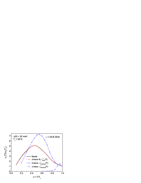
Figure 1: (Color online) Normalized microwave conductivity $\sigma_{1}(T)/\sigma_{1}(T_{c})$ vs reduced temperature $t$. The solid (black) line are the results from an Eliashberg calculation of Ref. Schachinger and Carbotte, 1998a which fit well experimental results (Ref. Bonn et al., 1994) for a twin-free optimally doped YBCO single crystal. The (red) open up-triangles represent our fit to the solid (black) curve using BCS $d$-wave with a temperature dependent scattering rate $\tau^{-1}_{\textrm{BCS}}(T)$. The open (blue) down-triangles connected by a dashed-dotted line are additional BCS $d$-wave results obtained now with the scattering rate $\tau^{-1}_{\textrm{TFM-BCS}}(T)$ derived from the two fluid model. Finally, the open (blue) down-triangles connected by the dotted line give the results of a BCS $s$-wave theory calculation using the scattering rate $\tau^{-1}_{\textrm{TFM-BCS}}(T)$.

Fig. 1 for the microwave frequency $34.8\,$GHz used in experiments.Bonn et al. (1994) The fit to the data is not shown here but it was very good. When the same model is applied to the London penetration depth an equally good fit to the data reported by D. A. Bonn et al.Bonn et al. (1993) was obtained and it is shown as the solid (black) line in Fig. 2 for the normalized square

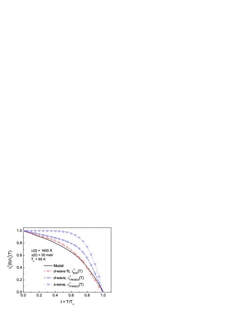
Figure 2: (Color online) The normalized inverse square of the penetration depth $\lambda^{2}_{L}(0)/\lambda^{2}_{L}(T)$ vs reduced temperature $t$. The solid (black) curve are results from an Eliashberg calculation (Ref. Schachinger et al., 1997) which fit well experimental results (Ref. Bonn et al., 1993) on an optimally doped YBCO single crystal. The open (red) up-triangles connected by a dashed line are the results of our BCS $d$-wave fit based on the scattering rate $\tau^{-1}_{\textrm{BCS}}(T)$. The open (blue) down-triangles connected by a dashed-dotted line are the result of a BCS $d$-wave calculation using the scattering rate $\tau^{-1}_{\textrm{TFM-BCS}}(T)$ derived from the two fluid model while the open (blue) down-triangles connected by a dotted line give the corresponding result of a BCS $s$-wave calculation.

of the penetration depth $\lambda^{2}_{L}(0)/\lambda^{2}_{L}(T)$ in optimally doped YBCO single crystals as a function of the reduced temperature $t$. The model also provides a good fit to corresponding thermal conductivity data.Schachinger and Carbotte (1998b)

In this paper we will use the solid (black) curves of Figs. 1 and 2 for microwave conductivity and penetration depth as representative of the cuprates and investigate whether or not a simpler formulation of microscopic theory, namely BCS theory, with a phenomenological temperature dependent scattering rate $\tau^{-1}_{\textrm{BCS}}(T)$ can also provide a good understanding of the data.

We begin with a fit to the microwave conductivity data of Fig. 1 [solid (black) line]. The open (red) up-triangles are our fit with the

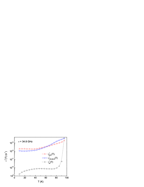
Figure 3: (Color online) Scattering rates $\tau^{-1}$ in inverse seconds as a function of temperature $T$ for an optimally doped YBCO single crystal. The scattering rate $\tau^{-1}_{\textrm{BCS}}(T)$ [open (red) up-triangles] was obtained by a BCS $d$-wave fit to the microwave conductivity [solid (black) line in Fig. 1] and Born impurity scattering. Finally, the (black) open squares present the optical scattering rate $\tau^{-1}_{\textrm{op}}(T)$, Eq. (13), at the microwave frequency $\nu$. Note, that in the normal state at $T=95\,$K the optical scattering rate is precisely twice the QP scattering rate $\tau^{-1}_{\textrm{BCS}}(T=95\,\textrm{K})$. The open (blue) down-triangles, finally, are the results of Eq. (12) as described in the text.

the corresponding quasiparticle scattering rate denoted $\tau^{-1}_{\textrm{BCS}}(T)$ shown as the open (red) up-triangles in Fig. 3. The fit is not unique and corresponds to a choice of least residual scattering at $T=0\,$, consistent with the normalized data of Fig. 1. This choice is partially motivated by the recognized fact that the cuprates are known to be rather pure. Other fits all would have larger values of $\tau^{-1}_{\textrm{BCS}}(T)$ at $T=T_{c}$ as well as residual impurity scattering at $T=0$. This ambiguity disappears if the plasma frequency $\Omega_{p}$ of Eq. (8) is known. As a first check on the validity of our phenomenological $\tau^{-1}_{\textrm{BCS}}(T)$ we can use it to calculate other properties. In Fig. 2 the (red) open up-triangles represent our results for the normalized inverse square of the penetration depth $\lambda^{2}_{L}(0)/\lambda^{2}_{L}(T)$ vs $T$. We see good, although not perfect agreement with the solid (black) curve. This demonstrates that a BCS approach with phenomenological $\tau^{-1}_{\textrm{BCS}}(T)$ fits to the microwave conductivity data cannot represent the penetration depth data which goes with it quite as accurately as we can with Eliashberg theory. Nevertheless, the fit is quite good and shows clearly that the simpler BCS approach used here can be applied with confidence to other systems such as the ferropnictides.

Moreover, one can define a TFM scattering rate based on our BCS calculation without reference to the plasma frequency $\Omega_{p}$. We define

$$\tau^{-1}_{\textrm{TFM-BCS}}(T)=\frac{1-\lambda^{2}_{L}(0)/\lambda^{2}_{L}(T)}{\sigma^{\prime}_{1}(T)},$$ (12)

where $\sigma^{\prime}_{1}(T)$ is in computer units defined without the factor $\Omega_{p}^{2}/(4\pi)$ in front of the right hand side of Eq. (8). Results are shown in Fig. 3 as the open (blue) down-triangles. The points cross the open (red) up-triangles for the quasiparticle scattering rate $\tau^{-1}_{\textrm{BCS}}(T)$ of BCS theory and show that the two scattering rates are not the same, they have a different temperature dependence. We might have expected them to differ only by a constant factor of two which is the relation expected to hold between optical and QP residual scattering rates. But this doesn’t hold here and shows the limitation of the concept of a TFM based scattering rate. We can even go further and use $\tau^{-1}_{\textrm{TFM-BCS}}(T)/2$ as an effective temperature dependent QP scattering rate in new BCS calculations. When this is done, we get the open (blue) down-triangles connected by a dashed-dotted line in Figs. 1 and 2 for the microwave conductivity and the penetration depth, respectively. The agreement with our model data [solid (black) line] is very poor. In particular, the peak in $\sigma_{1}(T)/\sigma_{1}(T_{c})$ is much higher in magnitude and occurs at higher values of the reduced temperature than in the model data. It is clear from this analysis that the scattering rate obtained from a TFM analysis cannot be used in BCS calculations to achieve a quantitative understanding of the data. Nevertheless, it still has some usefulness in that it allows one to understand qualitatively how the collapse of the inelastic scattering at low temperatures can result in a peak in the microwave conductivity at intermediate values of the reduced temperature $t$.

In Figs. 1 and 2 there is another set of open (blue) down-triangles connected by a dotted line. These were obtained in BCS calculations with $\tau^{-1}_{\textrm{TFM-BCS}}(T)/2$ as the QP scattering rate in Eqs. (6a) and (6b) but now the gap is assumed to have $s$-wave symmetry $(x=1)$. We see that this assumption has a drastic effect on both microwave conductivity and penetration depth when compared with similar results for a $d$-wave symmetric gap. In particular, the microwave conductivity does not show a peak at intermediate reduced temperatures and is already very small for $t=0.8$. This behavior is traced to the much more rapid drop in normal fluid density with decreasing $T$ in the $s$ than in the $d$-wave case. The first is exponentially small at $T\to 0$ while the other is linear in $T$ in the same limit. This has important implications for the data of Hashimoto et al.Hashimoto et al. (2009) in Ba_1-xK_xFe₂As₂ as we will elaborate upon in the next section.

Before turning to this discussion we make one final point about the pure isotropic $s$-wave case. In Fig. 4 we show results of

Figure 4: The normalized microwave conductivity $\sigma_{1}(T)/\sigma_{1}(T_{c})$ at $28\,$GHz vs temperature $T$ for an isotropic $s$-wave Eliashberg superconductor with the parameters noted in the figure and described in the text. The solid and dashed lines include residual impurity scattering $\tau^{-1}_{\textrm{imp}}$ of $4.75\times 10^{12}$ inverse seconds. A low frequency cutoff in the $\alpha^{2}F(\omega)$ spectrum of $\omega_{c}/T_{c}=2.2$ was applied to simulate the collapse of the inelastic scattering rate as $T\to 0$.

Eliashberg calculations with an MMP form for the electron-boson interaction as we employed to describe the inelastic scattering in YBCO but now an $s$-wave gap is used. The model parameters are $\omega_{SF}=30\,$ meV, the electron-spin fluctuation coupling strength $I^{2}$ was chosen to give an mass enhancement factor of $\lambda=1.64$, and the high energy cutoff $\omega_{D}$ of the spectrum was set to $200\,$meV. This resulted, together with the Coulomb pseudopotential $\mu^{\star}=0.1$ in a $T_{c}$ of $50\,$K more in line with the critical temperatures observed in the ferropnictides. Some elastic impurity scattering modeled by a constant value of the impurity scattering rate $\tau^{-1}_{\textrm{imp}}=4.75\times 10^{12}\,$s^-1 was also included. We note that the peak in the solid curve is at lower temperature and is much broader than the usual coherence peak of BCS theory. It also reacts to the addition of elastic impurity scattering (dashed-dotted curve) in the opposite way to conventional BCS.Marsiglio (1991) Increased impurity scattering depletes the magnitude of the peak, moves it to higher temperatures and narrows it considerably. These effects are the same as found in earlier work by Nicol and CarbotteNicol et al. (1991) based on the MFLM of Varma et al.Varma et al. (1989) The physics underlying the existence of the peak relates to scattering time variations and not to the classical coherence argument of BCS theory. What is important for the present paper is that the mechanism of the collapse in inelastic scattering is much less effective in producing peaks in the microwave conductivity for $s$-wave than it is for $d$-wave gap symmetry. The fundamental difference that accounts for this observation is that, in $s$-wave the normal fluid density drops to zero exponentially and becomes essentially negligible at low temperatures where the $d$-wave normal fluid density remains very significant.

We make a final point. While we discussed two different scattering rates $\tau^{-1}_{\textrm{TFM-BCS}}(T)$ and $\tau^{-1}_{\textrm{BCS}}(T)$ one can define others which can be useful in different contexts. For example, the extended Drude model is often used to define a temperature and frequency dependent optical scattering rate $\tau^{-1}_{op}(T,\omega)$ in terms of the complex optical conductivity, with

$$\tau^{-1}_{op}(T,\omega)=\frac{\Omega^{2}_{p}}{4\pi}\textrm{Re}\left[\sigma^{-1}(T,\omega)\right].$$ (13)

Evaluation of Eq. (13) for the microwave frequency $\nu=34.8\,$GHz gives the open (black) squares in Fig. 3 using our BCS model results. It is clear that $\tau^{-1}(T,\nu=34.8\,\textrm{GHz})$ is totally different from either $\tau^{-1}_{\textrm{BCS}}(T)$ or $\tau^{-1}_{\textrm{TFM-BCS}}(T)$. All play a role depending on the question asked.Schachinger and Carbotte (2003); Hensen et al. (1997); Schachinger and Carbotte (2000) Finally, we would like to note that just above $T_{c}$, $\tau^{-1}_{op}(T=95\,\textrm{K})$ and $\tau^{-1}_{\textrm{TFM-BCS}}(T=95\,\textrm{K})$ agree and are twice the $\tau^{-1}_{\textrm{BCS}}(T=95\,\textrm{K})$.

III Two Band $s^{\pm}$ superconducting state

The newly discoveredKamihara et al. (2008) layered ferropnictide superconductors display a complex band structureSingh and Du (2008) with several electron and hole like pockets crossing the Fermi energy. Multi-band superconductivity is now well establishedNicol and Carbotte (2005) in MgB₂ which is widely believed to be a conventional electron-phonon mechanism superconductor with two bandsChoi et al. (2002); Golubov et al. (2002); Jin et al. (2003) one with a large gap and the other much smaller. While in the ferropnictides there are more bands and the mechanism is not likely to be the electron-phonon interaction,Boeri et al. (2008) a minimum model that is often used is to include an electron band at the $M$ and a hole band centered at the $\Gamma$ points of the Brillouin zone with $s$-wave gaps of different magnitude with change in sign between the two referred to as $s^{\pm}$-symmetry.Mazin et al. (2008) Angular resolved photo emission spectroscopy (ARPES) in Ba_0.6K_0.4Fe₂As₂ by Ding et al.Ding et al. (2008) gives values $\Delta_{2}\simeq 12\,$meV and $\Delta_{1}\simeq 6\,$meV which were confirmed by Nakayama et al.Nakayama et al. (2009) Somewhat smaller values $\sim 9\,$meV and $\sim 4\,$meV are reported by the ARPES work of Evtushinsky et al.Evtushinsky et al. (2009) An important question which remains controversial is whether or not the $s$-wave gap on one of the Fermi surfaces can be sufficiently anisotropic to acquire a node or is it node-less.Chubukov et al. (unpublished); Yanagi et al. (2008); Kuroki et al. (2008); Wang et al. (2009); Graser et al. (2009) Large anisotropies of the $s$-wave gap are certainly expected even in conventional electron-phonon metals. Indeed multiple plane wave calculations of the electron-phonon spectral density $\alpha^{2}F(\omega)$ in Pb and Al,Tomlinson and Carbotte (1976); Leung et al. (1976a, b) and first-principle calculations of the electron-phonon contribution to the phonon linewidth in NbButler et al. (1979) found large anisotropies in this quantity and in the resulting superconducting gap values. Also in the high $T_{c}$ cuprates where the gap has $d$-wave symmetry calculations within a BCS spin fluctuation model with over-damped magnons as in the work of Millis et al.Millis et al. (1990) have produced gaps which go beyond the simplest $d$-wave versions with many higher harmonics and even leads to mixtures of $s$ and $d$-wave with profound effects on the resulting temperature dependence of the penetration depth.O’Donovan and Carbotte (1995); O’Donovan and Carbotte (1995a, b); Branch and Carbotte (1995) The penetration depth measurements in FeAs-122 of Hashimoto et al.Hashimoto et al. (2009) gave isotropic gaps with $\Delta_{2}\sim 6.8\,$meV and $\Delta_{1}\sim 3.3\,$meV, considerably smaller than ARPES but, nevertheless, implying an exponential activated behavior at low temperatures. In sharp contrast, measurements by Martin et al.Martin et al. (2009) found a non-exponential, close to $T^{2}$ law down to the lowest temperature measured ($T\sim 0.2\,T_{c}$). While muon-spin resonance experiments by Khasanov et al.Khasanaov et al. (unpublished) gives isotropic gaps with $\Delta_{2}\sim 9\,$meV and $\Delta_{1}\sim 1.5\,$meV we note that this second gap is becoming rather small. Heat transport measurements by Luo et al.Luo et al. (unpublished) are also consistent with no gap nodes but they indicate that the anisotropic $s$-wave gap may be quite small in certain momentum directions. Finally, we mention the nuclear spin magnetic resonance data for ⁵⁷Fe by Yashima et al.Yashima et al. (2009) which is consistent with $s^{\pm}$-symmetry with full gaps.

In Fig. 5(a) we show results of our two band BCS calculations

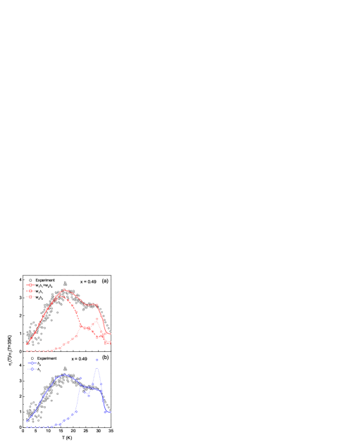
Figure 5: (Color online) (a) Two band $s^{\pm}$ fit to the normalized microwave conductivity $\sigma_{1}(T)/\sigma_{1}(T=35\,\textrm{K})$ of Ref. Hashimoto et al., 2009 (open circles) at the microwave frequency $\nu=28\,$GHz vs temperature. In our model the small gap $\Delta_{1}$ on the hole socket is assumed to be isotropic $s$-wave while the large gap $\Delta_{2}$ on the electron pocket includes anisotropy characterized by the parameter $x=0.49$ fixed to get a best fit to the data [open (red) squares connected by a solid line]. The contribution of the gap $w_{1}\Delta_{1}$ to the two band fit is shown by open (red) squares connected by a dotted line while the open (red) squares connected by a dashed line indicate the contribution of the second gap $w_{2}\Delta_{2}$. The corresponding scattering rate $\tau^{-1}_{\textrm{BCS}}(T)$ is shown by open (red) squares in the top frame of Fig. 6. (b) The same as the top frame but now for a fit to experiment using a single anisotropic $s$-wave gap $\Delta_{2}$ indicated by the open (blue) chevron connected by a solid line. The anisotropy parameter is $x=0.49$.

based on Eqs. (6) for the normalized microwave conductivity $\sigma_{1}(T)/\sigma_{1}(T=35\,\textrm{K})$ as a function of temperature $T$ for a microwave frequency $\nu=28\,$GHz. The open (black) circles indicate experimental results by Hashimoto et al.Hashimoto et al. (2009) for FeAs-122, sample #3 with $T_{c}=32.7\,$K. The open (red) squares connected by a solid line show the theoretical results which are seen to fit well the data even at low temperatures where the absorption appears to be roughly linear in $T$. The corresponding temperature dependent inelastic scattering rate $\tau^{-1}_{\textrm{BCS}}(T)$ is indicated by open (red) squares in the top frame of Fig. 6. The small gap $\Delta_{1}(0)$ on the hole surface was assumed to be isotropic $s$-wave and equal to $3.3\,$meV [$\Delta_{1}(0)/(k_{B}T_{c})=1.17$] while the larger gap of amplitude $\Delta_{2}(0)=6.8\,$meV [$\Delta_{2}(0)/(k_{B}T_{c})=2.4$] was allowed to be anisotropic of the form $\Delta_{2}(\theta)=\Delta_{sd}(\theta)=\Delta_{s}+\Delta_{d}\sqrt{2}\cos(2\theta)$. The contribution of the $s$-wave gap to $\Delta_{2}$ is determined by the parameter $x$ of Eq. (7). The $s^{\pm}$-model is defined by the combination of the two gaps $\Delta_{s^{\pm}}=w_{1}\Delta_{1}+w_{2}\Delta_{2}$.

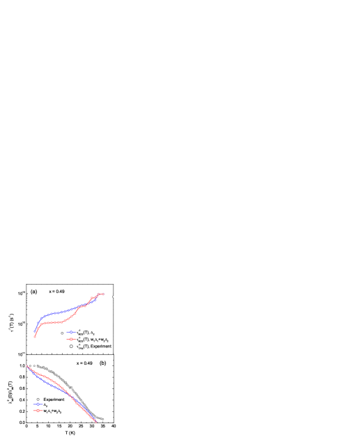
Figure 6: (Color online) (a) The inelastic scattering rate $\tau^{-1}_{\textrm{BCS}}(T)$ in inverse seconds obtained from our fits to the microwave conductivity data (Ref. Hashimoto et al., 2009) presented in Fig. 5. The open (red) squares correspond to the fit presented in the top frame of this figure while the open (blue) chevron correspond to the fit presented in the bottom frame. (b) The normalized inverse square of the penetration depth $\lambda^{2}_{ab}(0)/\lambda^{2}_{ab}(T)$ vs temperature $T$. The open (black) circles are the data for sample #3 of Ref. Hashimoto et al., 2009. The two curves indicated by open (red) squares and open (blue) chevron, respectively have been generated using BCS theory the temperature dependent inelastic scattering rates indicated by the same symbols in the top frame of this figure. The open circles are from the data of Table I of Ref. Hashimoto et al., 2009.

Furthermore, the complex conductivity $\sigma(T,\omega)=w_{1}\sigma^{(1)}(T,\omega)+w_{2}\sigma^{(2)}(T,\omega)$. Here $\sigma^{(1)}(T,\omega)$ and $\sigma^{(2)}(T,\omega)$ are the complex conductivities calculated using Eq. (8) for the two gapfunctions $\Delta_{1}(T,\omega)$ and $\Delta_{2}(T,\omega)$, respectively. In doing so we are assuming that the interband transitions can be ignored which is expected since the two $\sigma^{(i)}(T,\omega)$ originate from very different regions of momentum space. In agreement with Hashimoto et al.Hashimoto et al. (2009) the weights $w_{1}$ and $w_{2}$ have been chosen to be equal to 0.55 and 0.45, respectively. Finally, the anisotropy parameter $x$ was allowed vary to get the best fit to the microwave conductivity data over the whole temperature range and was found to be equal to 0.49. Thus, we have a 49% $s$-wave contribution to the big gap $\Delta_{2}$ which means that it has nodes on the Fermi surface although it is anisotropic $s$-wave.Schürrer et al. (1998) The open (red) squares connected by a dotted line and a dashed line give the individual contribution of $\Delta_{1}$ and $\Delta_{2}$, respectively, to the microwave conductivity. It is clear from this decomposition that it is the anisotropic gap with the nodes which contributes most at low temperatures as well as to the peak at $\sim 17\,$K. However, the hump around $30\,$K is due mainly, but not exclusively, to the small gap. Note with reference to Fig. 6(a) that the temperature dependent scattering rate obtained [open (red) squares] is very reasonable and equal to $9.5\times 10^{12}\,$s^-1 at $T_{c}$ and shows a residual scattering rate of $\tau^{-1}_{\textrm{BCS}}(T=1.6\,\textrm{K})=3.8\times 10^{11}\,$s^-1 indicating that sample #3 of Hashimoto et al.Hashimoto et al. (2009) is rather clean, so we do not expect impurities to significantly alter the symmetry of the gap. The open circles in Fig. 6(a) are the optical scattering rates given in Table I of Hashimoto et al.Hashimoto et al. (2009) obtained by a TFM analysis of their microwave conductivity supplemented with their penetration depth data on the same sample. As we found for the case of the cuprates $\tau^{-1}_{\textrm{TFM}}(T)$ is quite different from $\tau^{-1}_{\textrm{BCS}}(T)$ and is smaller by a significant amount. The open (blue) chevrons are to be compared with the open (red) squares and give the scattering rate according to BCS theory needed to fit the microwave conductivity data in FeAs-122 with a single anisotropic gap $\Delta_{2}$. The fit obtained is shown as the open (blue) chevrons connected by a solid line in Fig. 5(b) which nicely go through the experimental data (open circles). It is important to note that if the the same scattering rate $\tau^{-1}_{\textrm{BCS}}(T)$ that fits experiment with the single anisotropic gap $\Delta_{2}$ is used for the small isotropic $s$-wave gap $\Delta_{1}$ we get the open (blue) chevrons with the dotted line through them. This curve is mainly confined to the temperature region above $T=20\,$K and shows, once again, that the symmetry of the gap has a determining affect on the temperature variation of the resulting microwave conductivity.

Next we look at the temperature dependence of the normalized penetration depth $\lambda^{2}_{ab}(0)/\lambda^{2}_{ab}(T)$ for the two gap $s^{\pm}$-model which fits well the microwave conductivity of Fig. 5(a). Theoretical results are shown as the open (red) squares on Fig. 6(b) and are to be compared with the open circles which are the data for sample #3 of Hashimoto et al.Hashimoto et al. (2009) Once a temperature dependent scattering rate $\tau^{-1}_{\textrm{BCS}}(T)$ was fixed to fit the microwave conductivity there remained no adjustable parameter and, as one can see, the fit to the data is deficient in two ways. First of all, it is clear that the region near $T=0$ is not exponentially activated as the data indicate but is rather linear as one would expect from a gap with nodes. The data is certainly more consistent with a node-less $s$-wave gap. Secondly, the curve at higher temperatures falls quite a bit below the data. If we had considered a single anisotropic $s$-wave gap fit to the microwave conductivity data instead of our two $s^{\pm}$-model we would have obtained the open (blue) chevrons for the penetration depth which provide an even poorer over all fit. As we described in the previous section on the cuprates we do not expect even for a $d$-wave gap that we can fit equally well the penetration depth with the same scattering rate as determined from the fit to the microwave conductivity, but for FeAs-122, the main problem has to do with the fact that the anisotropy parameter $x=0.49$ obtained in the unconstrained fit, leads to a large gap $\Delta_{2}$ which has nodes.

A natural question to ask next is what would happen if instead of fitting the microwave conductivity we fit the penetration depth. In Fig. 7

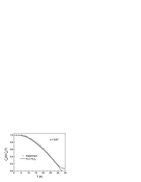
Figure 7: The normalized inverse square of the penetration depth $\lambda^{2}_{ab}(0)/\lambda^{2}_{ab}(T)$ vs temperature $T$. The open circles are the data for the FeAs-122 sample #3 of Ref. Hashimoto et al., 2009. The solid line represents the BCS fit to the data using our two band $s^{\pm}$-model with isotropic $s$-wave smaller gap $\Delta_{1}$ and an anisotropic larger gap $\Delta_{2}$ with the anisotropy parameter $x=0.67$ in the clean limit. The weights $w_{1}=0.55$ and $w_{2}=0.45$.

we consider the BCS clean limit and vary the anisotropy parameter $x$ to get a good fit to the data (open circles). For $x=0.67$ we get the solid line which is in very good agreement with experiment. It corresponds to the mixture $w_{1}\Delta_{1}+w_{2}\Delta_{2}$ of the two gaps in our $s^{\pm}$-model with $w_{1}=0.55$ and $w_{2}=0.45$. We proceed with these new $s^{\pm}$-model parameters to find a temperature dependent scattering rate to fit the microwave conductivity data. Our results are shown as

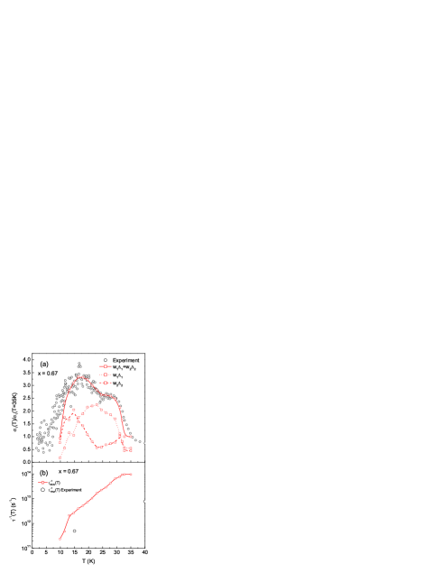
Figure 8: (Color online) (a) The normalized microwave conductivity $\sigma_{1}(T)/\sigma_{1}(T=35\,\textrm{K})$ for the FeAs-122 sample #3 of Ref. Hashimoto et al., 2009 at $\nu=28\,$GHz as a function of temperature $T$. The open (red) squares connected by a solid line are the best fit obtained within a two band $s^{\pm}$-band BCS theory with a temperature dependent scattering rate $\tau^{-1}_{\textrm{BCS}}(T)$ as to simulate the inelastic scattering. The smaller (hole band) gap is isotropic $s$-wave and the larger (electron band) gap is anisotropic $s$-wave with $x=0.67$ chosen to give a reasonable fit to the penetration depth data. (See Fig. 7.) The open (red) squares connected to the dashed and dotted lines give the individual contributions of the two gaps. (b) The inelastic scattering rate $\tau^{-1}(T)$ vs temperature. The open (red) squares give $\tau^{-1}_{\textrm{BCS}}(T)$, the inelastic scattering rate from our fit to the microwave conductivity shown in the top frame of this figure. The open circles represent data for the FeAs-122 sample #3 of Ref. Hashimoto et al., 2009.

the solid (red) squares connected by a solid line in Fig. 8(a). The over all fit is good including the region of the peak at $\sim 17\,$K. The main deficiency is that below $10\,$K where the theoretical curve drops sharply to zero while the experiment still gives absorption. There are two features of this fit we wish to emphasize. The open (red) squares connected by a dotted line give the separate contribution to the total from the small gap $w_{1}\Delta_{1}$ while the dashed curve with the open (red) squares is from the large, now node-less, anisotropic gap $w_{2}\Delta_{2}$. In contrast to what was observed in Fig. 5(a) where the large gap dominated the low temperature behavior and the small gap contributed mainly just below $T_{c}$ now both contributions extend over all temperatures with the small gap contribution still important at lowest temperatures and displaying a broad peak at $\sim 23\,$K. The BCS inelastic scattering rate obtained from this fit is given in Fig. 8(b) by open (red) squares. We note in comparison with the data of Fig. 6(a) that $\tau^{-1}_{\textrm{BCS}}(T=T_{c})$ is now much bigger and approximately equal to $1.9\times 10^{14}\,$s^-1. This is much bigger than the scattering rate derived from a TFM fit to the data by Hashimoto et al.Hashimoto et al. (2009) shown as the open circles. While $\tau^{-1}_{\textrm{BCS}}(T=T_{c})$ is to be interpreted as due to inelastic scattering it is rather big and indicates that this second fit to the microwave conductivity data while more compatible with the experimental penetration depth at low temperatures remains somewhat problematical.

Figure 9 presents a comparison between experimental results

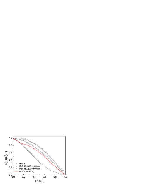
Figure 9: (Color online) The normalized inverse square of the penetration depth $\lambda^{2}_{ab}(0)/\lambda^{2}_{ab}(T)$ vs the reduced temperature $t$. The open circles represent the data by Hashimoto et al.Hashimoto et al. (2009) while the open down-triangles and open up-triangles give the results reported by Martin et al.Martin et al. (2009) for $\lambda_{ab}(0)$ equal to $180\,$nm and $600\,$nm, respectively. The open (red) squares correspond to our result of a BCS calculation in $s^{\pm}$ symmetry where the large gap $\Delta_{2}$ has nodes on the electronic Fermi surface [see also Fig. 6(b)].

of Hashimoto et al.Hashimoto et al. (2009) (open circles) and of Martin et al.Martin et al. (2009) [open down-triangles for $\lambda_{ab}(0)=180\,$nm and open up-triangles for $\lambda_{ab}(0)=600\,$nm]. Our result of a BCS $s^{\pm}$-symmetry calculation is indicated by the open (red) squares. They correspond to an anisotropic large gap $\Delta_{2}$ with nodes on the electronic Fermi surface and have already been discussed in Fig. 6(b). At low temperatures theory agrees well with the data by Martin et al.Martin et al. (2009) for $\lambda_{ab}(0)=180\,$nm. For higher temperatures theory is always above this data set but stays significantly below the data for $\lambda_{ab}(0)=600\,$nm. As $\lambda_{ab}(0)$ plays the role of a fitting parameter in the analysis of Martin et al.Martin et al. (2009) a $\lambda_{ab}\simeq 400\,$nm will probably bring experiment closer to theory. Nevertheless, the low temperature dependence of the penetration depth as reported by Martin et al.Martin et al. (2009) is certainly more in line with the microwave conductivity data of Hashimoto et al.Hashimoto et al. (2009) which shows a linear temperature dependence of $\sigma_{1}(T)/\sigma_{1}(T=35\,\textrm{K})$ below $T=10\,$K for $T\to 0$. Thus, at low temperatures there is still substantial absorption in the system which is in contradiction to the exponentially activated behavior observed by Hashimoto et al.Hashimoto et al. (2009) In a final point it is certainly important to note that the potassium content is quite different in the samples used in both experiments. Hashimoto et al.Hashimoto et al. (2009) report for their sample #3 $\sim 55\,$% potassium while Martin et al.Martin et al. (2009) report a potassium content of $\sim 30\,$% for their sample B.

IV Summary and conclusion

We have reexamined the use of the two fluid model as a way of extracting from a combination of microwave conductivity and penetration depth data a temperature dependent scattering rate $\tau^{-1}_{\textrm{TFM}}(T)$ which is believed to model the inelastic scattering. It has the very desirable property that, when it is multiplied into the normal fluid density, it reproduces the microwave conductivity. However, no test of its general validity has been provided. In this paper we take a different approach and use instead BCS theory to extract through a tight fit to the microwave conductivity a new temperature dependent inelastic scattering rate $\tau^{-1}_{\textrm{BCS}}(T)$. A comparison of $\tau^{-1}_{\textrm{BCS}}(T)$ with its TFM counterpart shows that they differ significantly both in absolute magnitude and in variation with $T$. This casts doubts on the quantitative significance of $\tau^{-1}_{\textrm{TFM}}(T)$. Nevertheless, the TFM does indeed provide a very useful basis for a first understanding of the role of inelastic scattering in those phenomena.

The fact that penetration depth information was not needed to extract our $\tau^{-1}_{\textrm{BCS}}(T)$ provides a first test of its validity. We use it in a BCS calculation with $d$-wave gap symmetry and find good semiquantitative agreement with the data in optimally doped YBCO, the same material used for the fit to the microwave conductivity. We take this small, yet significant discrepancy, as evidence that a temperature dependent but constant in frequency QP scattering rate does not capture all of the quantitative features of inelastic scattering. Because of the simplifications inherent in BCS theory a constant in frequency scattering rate is strictly required. But inelastic scattering intrinsically implies a frequency dependence to $\tau^{-1}(T,\omega)$ which is closely linked to its $T$ dependence. For instance for electron-phonon coupling the $\omega^{2}$ dependence of the spectral density $\alpha^{2}F(\omega)$ at small $\omega$ implies a $T^{3}$ law for the quasiparticle scattering rate at $\omega=0$ and also a $\omega^{3}$ law for $T=0$. Similarly, for the coupling to over-damped spin fluctuations as is the case in the nearly antiferromagnetic Fermi-liquid model of the cuprates the corresponding laws are $T^{2}$ and $\omega^{2}$. Furthermore, the frequency dependence of $\tau^{-1}(T,\omega)$ implies by Kramers-Kronig transform a nontrivial (i.e.: nonzero) real part of the quasiparticle self energy. It is precisely these features that are incorporated in the $d$-wave generalization of Eliashberg theory which we have used in our previous work. It is the results of our previous quantitative fit to microwave conductivity and penetration depth data in optimally doped YBCO single crystals that we have used here in our comparison with BCS. An important conclusion of all this is that Eliashberg theory is fully quantitative while BCS provides a good semiquantitative picture, its main limitation being due to the neglect of frequency dependence of the inelastic QP scattering rate.

Having established the validity of BCS theory to provide meaningful results in the present context we considered next its generalization to the two band case. This is the minimum model required for a realistic treatment of superconductivity in the ferropnictides in which there can be several hole and electron pockets with different values of the superconducting gap. A favored model is an $s^{\pm}$-model with isotropic $s$-wave gaps on each of the two bands and with opposite signs. We also consider the possibility that one of the gaps is anisotropic $s$-wave as in the work of Chubukov et al.Chubukov et al. (unpublished) and others.Wang et al. (2009) Anisotropy is expected even from consideration of conventional superconductivityGraser et al. (2009); Tomlinson and Carbotte (1976); Leung et al. (1976a, b); Butler et al. (1979) and also the cuprates.O’Donovan and Carbotte (1995); O’Donovan and Carbotte (1995a, b)

A general conclusion of our analysis is that with isotropic $s$-wave it is difficult to get realistic values of the quasiparticle scattering rate $\tau^{-1}_{\textrm{BCS}}(T)$ from microwave conductivity data which shows very significant absorption at low temperatures as is seen in the data of Hashimoto et al.Hashimoto et al. (2009) for FeAs-122. This is also the case when the big gap is allowed to be anisotropic but with no nodes on the Fermi surface. On the other hand, if the gap is sufficiently anisotropic to have nodes it becomes rather easy to get a fit to the FeAs-122 microwave conductivity data with realistic values of $\tau^{-1}_{\textrm{BCS}}(T)$. But a node on one of the gaps also leads to a penetration depth which shows $d$-wave like low temperature power laws (i.e.: linear in temperature) rather than the exponential activation behavior found experimentally on the same FeAs-122 sample which is the characteristic of a gap with finite value everywhere on the Fermi surface. On the other hand, the microwave conductivity data of Hashimoto et al.Hashimoto et al. (2009) is much more consistent with the more recent penetration depth data of Martin et al.Martin et al. (2009) on a related but not identical FeAs-122 sample.