Clustering based on Random Graph Model embedding Vertex Features

Abstract

Large datasets with interactions between objects are common to numerous scientific fields (i.e. social science, internet, biology…). The interactions naturally define a graph and a common way to explore or summarize such dataset is graph clustering. Most techniques for clustering graph vertices just use the topology of connections ignoring informations in the vertices features. In this paper, we provide a clustering algorithm exploiting both types of data based on a statistical model with latent structure characterizing each vertex both by a vector of features as well as by its connectivity. We perform simulations to compare our algorithm with existing approaches, and also evaluate our method with real datasets based on hyper-textual documents. We find that our algorithm successfully exploits whatever information is found both in the connectivity pattern and in the features.

, and

label=e1]hugo.zanghi@exalead.com label=e2]stevenn.volant@agroparistech.fr label=e3]christophe.ambroise@genopole.cnrs.fr label=u]http://www.exlead.com

1 Introduction

Classical data analysis has been developed for sets of objects with features, but when explicit relationships exist between objects, classical data analysis cannot take these relations into account. On the other hand, much recent research has been performed for analyzing graphs, for example in finding relationships in social sciences, gene interactions in biology and hyperlinks analysis in computer science, providing insights into the interactions in these networks. Many approaches to graph analysis have been proposed. Model-based approaches, i.e., methods which rely on a statistical model of network edges and vertices, such as those first proposed by Erdös-Rényi , often allow to get insight into the network structure deducing their internal properties.

An interesting alternative to the basic Erdös-Rényi model which does not fit well to real networks is to consider a mixture of distributions (Frank & Harary, 1982; Snijders & Nowicki, 1997; Newman & Leicht, 2007; Daudin et al., 2008) where it is assumed that nodes are spread among an unknown number of latent connectivity classes. Conditional on the hidden class label, edges are still independent and Bernoulli distributed, but their marginal distribution is a mixture of Bernoulli distributions with strong dependence between the edges. Many names have been proposed for this model, and in the following, it will be denoted by MixNet, which is equivalent to Block Clustering of Snijders & Nowicki (1997). Block-Clustering for classical binary data can be dated back to early work in the seventies (Lorrain & White, 1971; Govaert, 1977).

But vertex content is also sometimes available in addition to the network information used in the methods mentioned above. A typical example is the world-wide-web which can be described by either hyperlinks between web pages or by the words occurring in the web pages: each vertex represents a web page containing the occurrences of some words and each directed edge a hyperlink. The additional information represented by the vertex features is rarely used in network clustering but can provide crucial information. Here we combine information from both vertex content traditionally used in classical data analysis to information found in the graph structure, in order to cluster objects into coherent groups. This paper proposes a statistical model, called CohsMix (for Covariates on hidden structure using Mixture models), which considers the dependent nature of the data and the relation with vertex features (or covariates) in order to capture a hidden structure.

Considering spatial or relational data neighbourhood is not an original approach in clustering. For instance, Hidden Markov Random Fields (HMRF) are well adapted to handle spatial data and are widely used in image analysis. When the spatial network is not given it is generally obtained using Delaunay triangulation (Ambroise et al., 1997).

Hoff (2003) proposed a new way to deal with covariates. He suggested to model the expected value of the relational ties by a logistic regression. The problem of this method is the dependence between the observations conditional on the regression parameters and the covariates. Hence, he proposed to incorporate random effect structures in a generalized linear model setting. The distribution of dependence among the random effects determines the dependence among the edges.

There are also approaches based on non statistical frameworks. In particular, it is noticeable that there exits a strong similitude between multiple view and graph models with covariates. In fact, multiple view learning algorithms (Ruping & Scheffer, 2005) consider instances which have multiple representations and simultaneously exploit these views to find a consensus partition.

The second section introduces the proposed model, which is an extension to the MixNet model. Since the model considers a great number of dependencies, the proposed estimation scheme proposes a variational approach of the EM algorithm. This approach allows us to deal with larger network than the Bayesian framework. Then we introduce practical strategies for the initialization and the choice of the number of groups. In the third section extensive simulations illustrate the efficiency of the this algorithm and real datasets dealing with hyper-textual documents are studied. A R package named CohsMix is available upon request.

2 A Mixture of Network with covariates

This section introduces the proposed model. We choose to consider a model which assumes independence of covariates and edges conditional on the node classes. It assumes that both the connectivity pattern and the vertex features can be explained by the class. In the web context this model considers that a given class contains documents which have both a similarity between occurring words and a similarity of connectivity pattern with documents inside and outside the class. Although this assumption does not explicitly model the idea that authors tend to link similar topics (occurring words) which creates a thematic locality (Davison, 2000), it allows us to detect clusters of local theme. Its simplicity makes it a robust well adapted model to the real web.

2.1 Models and Notation

Let us define a random graph $G$, where $\mathcal{V}$ denotes the set of vertices. Based on the MixNet model, our model assumes that $\mathcal{V}$ is partitioned into $Q$ hidden classes. Let us denote by $Z_{iq}$ the indicator variable such that $\{Z_{iq}=1\}$ if node $i$ belongs to class $q$. ${\bf Z}=({\bf Z}_{1},\ldots,{\bf Z}_{n})$ is the vector of random independent indicator variables such that

$${\bf Z}_{i}\sim{\cal M}(1,\mbox{{$\alpha$}}=\{\alpha_{1},...,\alpha_{Q}\}),$$ (1)

with $\alpha$ the vector of class proportions. Edges are Bernoulli random variables

$$X_{ij}|{Z_{iq}Z_{jl}=1}\sim\mathcal{B}(\pi_{ql}),$$ (2)

conditionally independent, given the node classes

$$P({\bf X}|{\bf Z})=\prod_{ij}\prod_{q,l}P(X_{ij}|Z_{iq}Z_{jl}=1)^{Z_{iq}Z_{jl}}.$$

In this paper, we consider an undirected graph we suppose that there is no self-loops, i.e. a node can not be connected to itself ($X_{ii}$ = 0). Nevertheless, the method can easily be generalized to encompass directed graphs with self-loops.

Vertex Features.

Hereafter we consider $n$ objects described both by their connections and $p$ features. In that case the data under study can be represented into different forms. One might for example consider a two part vector for characterizing each object, where the first part contains the feature of the object $\mathbf{Y}_{i}$ and the second part contains a binary vector representing the connection to all $n-1$ other objects $\mathbf{X}_{i}$. Continuing our example about world-wide-web, the web pages can be viewed as a vector of word occurrences with hyperlinks or as two matrices. One based on the adjacency matrix describing the topology of the graph generated by the hyperlinks and the other by the features matrix generated by the word occurrences in each web page.

Hereafter we consider that the $p$ dimensional feature vector associated to object $i$ is defined by :

$$\mathbf{Y}_{i}=\left(\begin{array}[]{cccc}Y^{(1)}_{i}\\ Y^{(2)}_{i}\\ \vdots\\ Y^{(p)}_{i}\\ \end{array}\right)$$

We assume that the feature vectors $\mathbf{Y}_{i}$ are multivariate normally distributed

$$\mathbf{Y}_{i}|Z_{iq}=1\sim\mathcal{N}(\boldmath{\mu}_{q},\Sigma_{q})$$ (3)

where

$\boldmath{\mu}_{q}=\left(\begin{array}[]{cccc}\mu^{(1)}_{q}\\ \mu^{(2)}_{q}\\ \vdots\\ \mu^{(p)}_{q}\\ \end{array}\right)$ and $\mathbf{\Sigma_{q}}=\sigma I$ the covariance matrix is proportional to the identity.

The random feature vectors $\mathbf{Y}_{i}$ are conditionally independent, given the node classes

$$P(\mathbf{Y}|\mathbf{Z})=\prod_{i}\prod_{q}P(\textbf{Y}_{i}|Z_{iq})^{Z_{iq}}.$$

The conditional distribution associated to covariates can be written as follow :

$$\log P(\mathbf{Y}|\mathbf{Z}) = \sum_{i}\sum_{q}Z_{iq}\log P(\mathbf{Y}_{i}|Z_{iq})$$

$$= \sum_{i}\sum_{q}Z_{iq}\left[\left(\log\frac{1}{2\pi^{\frac{n}{2}}det(\Sigma)^{\frac{1}{2}}}\right)-\frac{1}{2}(\textbf{Y}_{i}-\boldmath{\mu}_{q})^{T}\sigma^{-1}(\textbf{Y}_{i}-\boldmath{\mu}_{q})\right].$$

The proposed mixture model assumes independence of $\mathbf{X}$ and $\mathbf{Y}$ conditional on $\mathbf{Z}$. Considering this independence between edges and covariates, the complete log-likelihood can be written as (Figure 1):

$$P(\mathbf{X},\mathbf{Y},\mathbf{Z})=P(Z)P(\mathbf{X},\mathbf{Y}|Z) = P(\mathbf{Z})P(\mathbf{Y}|\mathbf{Z})P(\mathbf{X}|\mathbf{Z}).$$

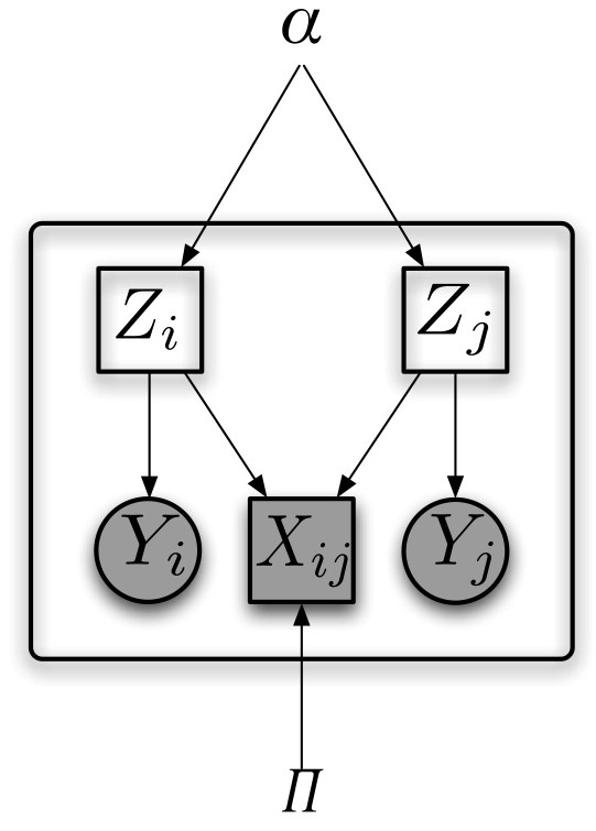
Figure 1: Graphical representation of the CohsMix Model. The squares represent discrete random variables and circles continuous random variables.

The next section proposes an estimation scheme for the CohsMix model.

2.2 Variational EM algorithm for CohsMix

In the classical em framework developed by Dempster et al. (1977), where $\mathbf{X}$ and $\mathbf{Y}$ are the available data, the inference of the unknown parameters $\mathbf{\Theta}$ spread over a latent structure $\mathbf{Z}$ uses the following conditional expectation:

$$Q\left(\mathbf{\Theta}|\mathbf{\Theta}^{(m)}\right)=\mathbb{E}\left\{\log\mathcal{L}_{c}(\mathbf{X},\mathbf{Y},\mathbf{Z};\mathbf{\Theta})\big{|}\mathbf{X},\mathbf{Y};\mathbf{\Theta}^{(m)}\right\}\\ =\sum_{\mathbf{Z}\in\mathcal{Z}}\mathbb{P}\left(\mathbf{Z}\big{|}\mathbf{X},\mathbf{Y};\mathbf{\Theta}^{(m)}\right)\log\mathcal{L}_{c}(\mathbf{X},\mathbf{Y},\mathbf{Z};\mathbf{\Theta})$$ (4)

where

$$\mathbf{\Theta^{(m+1)}}=\displaystyle{\mathop{\mathrm{Argmax}}_{\mathbf{\Theta}}}Q(\mathbf{\Theta},\mathbf{\Theta}^{(m)}).$$

The usual em strategy would be to alternate an E-step computing the conditional expectation (4) with an M-step maximizing this quantity over the parameter of interest $\mathbf{\Theta}$. Unfortunately, no closed form of $Q\left(\mathbf{\Theta}|\mathbf{\Theta}^{(m)}\right)$ can be formulated in the present case. The technical difficulty lies in the complex dependency structure of the model. Indeed, $\mathbb{P}(\mathbf{Z}|\mathbf{X},\mathbf{Y};\mathbf{\Theta})$ cannot be factorized, as argued in Daudin et al. (2008). This makes the direct calculation of $Q\left(\mathbf{\Theta}|\mathbf{\Theta}^{(m)}\right)$ impossible. To tackle this problem we use a variational approach (see, e.g., Jordan et al., 1999, for elementary results on variational methods). In this framework, the conditional distribution of the latent variables $\mathbb{P}(\mathbf{Z}|\mathbf{X},\mathbf{Y};\mathbf{\Theta}^{(m)})$ is approximated by a more convenient distribution denoted by $R(\mathbf{Z})$, which is chosen carefully in order to be tractable. Hence, our em-like algorithm deals with the following approximation of the conditional expectation (4)

$$\mathbb{E}_{R}\left\{\log\mathcal{L}(\mathbf{X},\mathbf{Y},\mathbf{Z};\mathbf{\Theta})\right\}=\sum_{\mathbf{Z}\in\mathcal{Z}}R(\mathbf{Z})\log\mathcal{L}(\mathbf{X},\mathbf{Y},\mathbf{Z};\mathbf{\Theta}).$$ (5)

In the following section we develop a variational argument in order to choose an approximation $R(\mathbf{Z})$ of $\mathbb{P}(\mathbf{Z}|\mathbf{X},\mathbf{Y};\mathbf{\Theta}^{(m)})$. This enables us to compute the conditional expectation (5) and proceed to the maximization step.

2.3 Variational estimation of the latent structure(E-step)

In this part, $\mathbf{\Theta}$ is assumed to be known, and we are looking for an approximate distribution $R(\cdot)$ of the latent variables. The variational approach consists in maximizing a lower bound $\mathcal{J}$ of the log-likelihood $\log\mathbb{P}(\mathbf{X},\mathbf{Y};\mathbf{\Theta})$, defined as follows:

$$\mathcal{J}\left(\mathbf{\Theta}\right)=\log\mathbb{P}(\mathbf{X},\mathbf{Y};\mathbf{\Theta})-\mathrm{D}_{KL}\left\{R(\mathbf{Z})\|\mathbb{P}(\mathbf{Z}|\mathbf{X},\mathbf{Y};\mathbf{\Theta}^{(m)})\right\}$$ (6)

where $\mathrm{D}_{KL}$ is the Küllback-Leibler divergence. This measures the difference between the probability distribution $\mathbb{P}(\cdot|\mathbf{\Theta})$ in the underlying model and its approximation $R(\cdot)$. An intuitively straightforward choice for $R(\cdot)$ is a completely factorized distribution (see Mariadassou & Robin, 2007; Zanghi et al., 2008)

$$R(\mathbf{Z})=\prod_{i\in\mathcal{P}}h_{\boldsymbol{\tau}_{i}}(\mathbf{Z}_{i}),$$ (7)

where $h_{\boldsymbol{\tau}_{i}}$ is the density of the multinomial probability distribution $\mathcal{M}(1;\boldsymbol{\tau}_{i})$, and $\boldsymbol{\tau}_{i}=(\tau_{i1},\dots,\tau_{iQ})$ is a random vector containing the variational parameters to optimize. The complete set of parameters $\boldsymbol{\tau}=\left\{\tau_{iq}\right\}_{i\in\mathcal{P},q\in\mathcal{Q}}$ is what we are seeking to obtain via the variational inference. In the case in hand the variational approach intuitively operates as follows: each $\tau_{iq}$ can be seen as an approximation of the probability that vertex $i$ belongs to cluster $q$, conditional on the data, that is, $\tau_{iq}$ estimates $\mathbb{P}(Z_{iq}=1|\mathbf{X},\mathbf{Y};\mathbf{\Theta})$, under the constraint $\sum_{q}\tau_{iq}=1$. In the ideal case where $\mathbb{P}(\mathbf{Z}|\mathbf{X},\mathbf{Y};\mathbf{\Theta})$ can be factorized as $\prod_{i}\mathbb{P}(\mathbf{Z}_{i}|\mathbf{X},\mathbf{Y};\mathbf{\Theta})$ and the parameters $\tau_{iq}$ are chosen as $\tau_{iq}=\mathbb{P}(Z_{iq}=1|\mathbf{X},\mathbf{Y};\mathbf{\Theta})$, the Küllback-Leibler divergence is null and the bound $\mathcal{J}$ reaches the log-likelihood.

The lower bound $\mathcal{J}$ to be maximized in order to estimate $\boldsymbol{\tau}$ can be expressed as

$$\mathcal{J}_{\boldsymbol{\tau}}=\mathbb{E}_{R(Z)}\left\{\mathcal{J}(\mathbf{\Theta})\right\}=\mathbb{E}_{R(Z)}\{\log(P(\mathbf{X},\mathbf{Y},\mathbf{Z}))|\mathbf{X},\mathbf{Y};\mathbf{\Theta}\}-\displaystyle{\sum_{Z}}R(\mathbf{Z})\log(R(\mathbf{Z})).$$

The optimal approximate distribution $R$ is then derived by direct maximization of $\mathcal{J}_{\boldsymbol{\tau}}$. Let all the parameters $\hat{\pi}_{ql},\hat{\alpha}_{q},\hat{\boldmath{\mu}}_{q}$ and $\hat{\sigma}$ be known. The following fixed-point relationship holds for the optimal variational parameters $\widehat{\boldsymbol{\tau}}=\arg\max_{\boldsymbol{\tau}}\mathcal{J}_{\boldsymbol{\tau}}$.

$$\hat{\tau}_{iq}^{(m+1)}\propto\hat{\alpha}_{q}\displaystyle{\prod_{j\neq i}\prod_{l}}\left[\hat{\pi}_{ql}^{x_{ij}}(1-\hat{\pi}_{ql})^{1-x_{ij}}\right]^{\tau_{jl}^{(m)}}\prod_{k=1}^{p}\left[\exp(\frac{1}{2\hat{\sigma}^{2}}\left(-(Y_{i}^{(k)}-\hat{\boldmath{\mu}}_{q}^{(k)})\right)^{2})\right].$$ (8)

Once again, the maximization of $\mathcal{J}_{\boldsymbol{\tau}}$ provides the optimal values of the parameters. The optimal parameters $\alpha_{q},\pi_{ql},\boldmath{\mu}_{q}$ and $\sigma$, i.e. the parameters maximizing $\mathcal{J}_{\boldsymbol{\tau}}$ satisfy the following relations:

$$\hat{\alpha}_{q} =\frac{1}{n}{\sum_{i=1}^{n}}\tau_{iq},$$ (9)

$$\hat{\pi}_{ql} =\frac{\displaystyle{\sum_{i\neq j}}\tau_{iq}\tau_{jl}x_{ij}}{\displaystyle{\sum_{i\neq j}}\tau_{iq}\tau_{jl}},$$

$$\hat{\mu}_{q} =\frac{\displaystyle{\sum_{i}}\tau_{iq}\mathbf{Y}_{i}}{\displaystyle{\sum_{i}}\tau_{iq}}\ \ \mbox{and}\ \ \hat{\sigma} =\frac{\displaystyle{\sum_{i}}\displaystyle{\sum_{q}}\tau_{iq}(\mathbf{Y}_{i}-\hat{\zeta}_{q})^{T}(\mathbf{Y}_{i}-\hat{\zeta}_{q})}{\displaystyle{\sum_{i}}\displaystyle{\sum_{q}}\tau_{iq}}.$$

For completeness, we summarize the variational EM algorithm for CohsMix in the Algorithm 1.

Data: Matrices of connectivities $\mathbf{X}$ and similarities $\mathbf{Y}$

/* Initialization of the parameters */

$\mathbf{\Theta}^{(0)}=\left(\alpha_{1}^{(0)},...,\alpha_{Q}^{(0)},\pi_{11}^{(0)},...,\pi_{QQ}^{(0)},\boldmath{\mu}_{1}^{(0)},...,\mu_{p}^{(0)},\sigma^{(0)}\right),m=0$

while not convergence do  /* Estimation step */

/* Compute $\boldsymbol{\tau}=\left\{\tau_{iq}\right\}_{i\in\mathcal{P},q\in\mathcal{Q}}$ the probabilities that vertex $i$ belong to cluster $q$ finding fix point of $g()$ */

foreach $i\in\{1,...,N\}$ do  foreach $q\in\{1,...,Q\}$ do  $\tau_{iq}^{(m+1)}=g(\boldsymbol{\tau}^{(m)})$ (see Equation 8)

  /* normalize posterior probabilities */

$scale=\sum_{q=1}^{Q}\tau_{iq}$

$\tau_{iq}=\tau_{iq}\frac{1}{scale}$, $\forall q\in\{1,...,Q\}$

  /* Maximization step */

/* re-estimate the distribution parameters to maximize the likelihood of the data */

Update parameters according Equation 9 :

foreach $q\in\{1,...,Q\}$ do  $\alpha_{q}^{(m+1)}=\mathop{\mathrm{Argmax}}_{\alpha_{q}}\mathcal{J}_{\boldsymbol{\tau}}(\mathbf{\Theta})$

foreach $l\in\{1,...,Q\}$ do  $\pi_{ql}^{(m+1)}=\mathop{\mathrm{Argmax}}_{\pi_{ql}}\mathcal{J}_{\boldsymbol{\tau}}(\mathbf{\Theta})$

$\mu_{q}^{(m+1)}=\mathop{\mathrm{Argmax}}_{\boldsymbol{\mu_{q}}}\mathcal{J}_{\boldsymbol{\tau}}(\mathbf{\Theta})$

    m = m +1

  Result: Estimated parameters $\mathbf{\Theta}$ and posterior probabilities $\tau_{iq}$

Algorithm 1 Variational EM CohsMix Algorithm

2.4 Model selection: ICL algorithm

As the number of clusters is an unknown parameter of our statistical model, it is possible to use the Integrated Classification Likelihood (ICL) to choose the optimal number of classes (Biernacki et al., 2000). The ICL criterion is essentially derived from the ordinary BIC considering the complete log-likelihood instead of the log-likelihood. This optimal number is obtained by running our algorithm concurrently for models from 2 to Q classes and selecting the solution which maximizes the ICL criterion. In our situation where additional covariates are considered, the ICL criterion can be written as:

$$ICL(Q) = \max_{\mathbf{\Theta}}\log\mathcal{L}(\mathbf{X},\mathbf{Y},\mathbf{Z};\mathbf{\Theta},Q)-\underbrace{\frac{1}{2}\times Q(Q-1)\log(\frac{n(n-1)}{2})}_{\mbox{\footnotesize{related to $\pi_{ql}$}}}-\underbrace{\frac{Q-1}{2}\log(n)}_{\mbox{\footnotesize{related to $\alpha_{q}$}}}$$

$$-\underbrace{p(p-1)\log(\frac{n(n-1)}{2})+p\times Q\log(\frac{n(n-1)}{2})}_{\mbox{\footnotesize{related to $\boldmath{\mu}_{q}$ \mbox{and} $\sigma$}}}$$

This expression of the ICL criterion is based on the method described in Daudin et al. (2008).

3 Experiments

In this section, we report experiments in order to assess the performances and limitations of the proposed model in a clustering context. We consider synthetic data generated according to the assumed random graph model, as well as real data from the web. Using synthetic graphs allows us to evaluate the quality of the parameter estimation. In parallel, we also compare classification results with alternative clustering methods using a ground truth. The real datasets consist of hypertext documents retrieved from a websearch query. A R package named CohsMix is available upon request.

3.1 Comparison of algorithms

Simulations set-up

In these experiments, we consider simple affiliation models with two parameters defining the probability of connection between nodes of the same class and of different classes, respectively $\pi_{qq}=\lambda$ and $\pi_{ql}=\epsilon$ and equal mixture proportion $\alpha_{1}=...=\alpha_{Q}=\frac{1}{Q}$. We consider models with $n=150$ nodes.

We generate graph models in order to evaluate the algorithm performances as the difficulty of the problem varies. The clustering problem increases in difficulty with the number of classes $Q$, the number of features $nbCov$, $d(\lambda,\epsilon)$ the euclidean distance between intra and extra connectivity parameters and $d(\mu_{q},\mu_{l})$ the distance between the feature mean vectors of classes. We decide to focus on these parameters to produce data with different levels of structure and eventually consider 43 different graph models whose description are summarized in Table 1. Each model is simulated 20 times.

Experiments	$Q$	$nbCov$	$d(\lambda,\epsilon)$	$d(\mu_{q}^{(j)},\mu_{l}^{(j)})$
a	$\{2,...,12\}$	3	0.4	4
b	5	$\{2,...,15\}$	0.2	4
c	3	3	$\{0,...,0.5\}$	4
d	3	3	0	$\{4,...,8.5\}$

Table 1: Parameters of the four different settings which are used to generate the 43 affiliation models considered in the experiments.

We use the adjusted Rand Index (Hubert & Arabie, 1985) to evaluate the agreement between the estimated and the actual partition. The Rand index is based on a ratio between the number of node pairs belonging to the same and to different classes when considering both partitions. It lies between 0 and 1, two identical partitions having an adjusted Rand Index equal to 1.

To avoid initialization issues, the algorithm is started with multiple initialization points and the best result is selected based on its likelihood. Thus, for each simulated graph, the algorithm is run 10 times and the number of clusters is chosen using the Integrated Classification Likelihood criterion, as proposed in the previous section.

Alternative clustering methods

Additionally to the CohsMix algorithm study, we compared it with two ”rivals” : a multiple view learning algorithm (Ruping & Scheffer, 2005; Zhang et al., 2006), and a Hidden Markov Random Fields (Ambroise et al., 1997):

• Spectral Multiple View Learning (SMVL) : There exits a strong similitude between multiple view and graph models with covariates. In fact, multiple view learning algorithms consider instances which have multiple representations and simultaneously exploit these views to find a consensus partition. This is achieved via spectral clustering on a linear combination of a standard kernel corresponding to the graph structure and a kernel corresponding to vertex proximity.

• Hidden Markov Random Fields (HMRF) : Hidden Markov Random Fields are commonly used to handle spatial data and are widely used in image analysis. We use a classical Potts model on the latent structure which encourage spatial smoothing of the cluster. This kind of approach uses the graph structure to smooth the partition of the vertex over the graph, whereas the approach proposed in this paper uses the graph structure directly to estimate the vertex partition.

Simulations results

We focus our attention on the Rand Index for each algorithm. Indeed, a well estimated partition leads to good estimates.

As expected, the performance of the three algorithms decrease with the number of groups (Figure 2 a).

A first interesting result is that, in presence of a modular structure (Figures 2 a,b and c) in the network and weakly informative features, CohsMix algorithms always performs better than SMLV and HMRF algorithms.

Besides, it is noticeable that performances of CohsMix increase with the number of features and/or with the distance between mean vectors (Figure 2 b and d). HMRF algorithm with Potts a priori use the neighborhood structure for smoothing the partition. A vertex with all its neighbors of a given class has a high probability to be assigned to this class but HRMF does not take advantage of the graph structure as fully as Cohsmix. Our model is thus mainly attractive and suitable for datasets with an existing graph structure.

When there is no graph structure at all and few informative features (Figure 2 d ) the Cohsmix does not compare to HMRF or SMLV. The Cohsmix algorithm is more sensitive to the total absence of graph structure than its competitor.

But in all other setup, the quality of partition estimation remains good with different kind of models, the CohsMix algorithm appears very attractive and suitable for structured graphs with vertex features. We shall see in the next section that this algorithm also performs well on real web datasets.

(a)	(b)
(c)	(d)

Figure 2: Comparison of HMRF, Spectral MLV and CohsMix. (a) Varying $Q$ the number of classes. (b) Varying the number of Features. (c) Varying the distance between intra and inter connectivity parameters. (d) Varying the distance between the mean vector of the classes.

3.2 Real data

Exhaustivity is an essential feature for information retrieval systems like Web search engines. However, it appears that ambiguous queries produce such a huge diversity in the responses that it is a real impediment to understanding. A common way to circumvent this situation is to organize search results into groups (clusters), one for each meaning of the query. This concern has been in the focus of the information retrieval community (Hearst & Pedersen, 1996; Zamir & Etzioni, 1998) since the early days of the Web. More recently, academic (Zeng et al., 2004) and industrial (Bertin & Bourdoncle, 2002) (exalead.com or clusty.com) attempts have made the clustering of search results a common feature for a WWW user.

The main drawback of many Web page clustering methods is that they take into account only the topical similarity between documents in the ranked list and they do not consider the topology induced by hyperlinks. But in competitive or controversial queries like ”abortion” or ”Scientology” such methods do not reveal community information that is visible on the link topology : By affinity, authors tend to link to pages with similar topics or points of view which create a thematic locality (Davison, 2000). In addition, ambiguous queries like ”orange” or ”jaguar” can also benefit from the link topology to produce more accurate separation of results. Combination of topological and topical clustering methods is a proven strategy to build an relevant system. One of the most relevant previous work is suggested in He et al. (2002), which build a Web page clustering system which accounts for the hyperlinks structure of the Web, considering two Web pages to be similar if they are in parent/child or sibling relations in the Web graph. A more general multi-agent framework based on path between each pair of results has been proposed by Bekkerman et al. (2006), but these methods, not model-based, use various heuristics and fine tunings.

Datasets setup

We use exalead.com search engine in our real data experiments. For each query, we retrieve the first 150 search results in order to build our graph and feature structures. Indeed, the web is a very sparse graph and thematic subgraphs may amplify this property creating unconnected components which inhibits the opportunity to use classical graph clustering algorithms directly on the observed adjacency matrix. In order to increase the graph density, the probability to have a link between two nodes, we propose to use the site graph of exalead.com basically based on the concepts of Raghavan & Garcia-Molina (2003). In this graph, nodes represent websites (a website contains a set of pages) and edges represent hyperlinks between websites. Multiple links between to different website are collapsed into a single link. Intra-domain links are taken into account if hostnames/websites are not similar. This site graph is previously computed. This methodology is similar to the Exalead application called Constellations : constellations.labs.exalead.com.

Then, text features are extracted from the content of the web page returned by the search engine. The features are built using various text processing like normalization, tokenization, entities detection, noun phrase detection and related terms detection. Besides, we remove rare features which do not appear more than twice. Eventually each feature vector is approximately of dimension $p=100$ and summarizes all text of a returned page.

Algorithm results.

We choose one ambiguous query (”jaguar”) and one controversial query (”Scientology”) to illustrate our algorithm behavior with real datasets. In Figure 3 associated to the query ”Scientology”, we can observe a well structured graph which fits our estimated latent partition with an optimal number of classes $Q=3$. Basically this partition yields the pro- and anti-Scientology clusters and identifies a gateway cluster (composed for example by http://en.wikipedia.org/wiki/Scientology) bridging the pro and anti cluster. Then, we concentrate our attention on the most representative text features of each class $q$. To succeed, we select the best occurrence of term features in the different $\mu_{q}$. Once again (see 3), we notice terms describing pro- like (”self esteem or ”providing real solutions”) and anti- like (”criticism of dianetics” or ”truth about Scientology”). The interface class is composed by common terms describing the church of Scientology. Thus, in a web context, the CohsMix algorithm is enable to named the different found partitions which a precious assistance to have rapidly a global overview of the hidden structure.

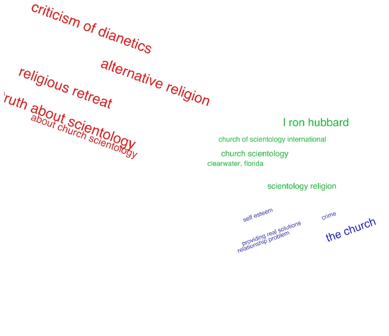
Figure 3: Representation of the results of a clustering of the webpages returned by the controversial query ”Scientology” using CohsMix. The graph structure is represented on the left and on the right are the main features. Colors indicate the CohsMix classification

The results of the processing of the ambiguous query ”jaguar” is represented in Figure 4. CohsMix clearly identifies three contexts: computer, animal and car model related web pages.

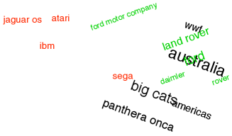
Figure 4: Representation of the results of a clustering of the webpages returned by the ambiguous query ”jaguar”.

The above results illustrate that our algorithm CohsMix seems well adapted to detect ambiguous or controversial queries of WWW search engine users.

4 Conclusion

This paper has proposed an algorithm for clustering dataset whose modelisation could be a graph structure embedding vertex features. Characterizing each vertex both by a vector of features as well as by its connectivity, CohsMix algorithm, based on a variational approach of EM, uses both elements to cluster the data and estimate the model parameters. When analyzing simulation and comparison results, our algorithm appears very attractive and competitive for various kind of models. We have tested CohsMix algorithm to cluster web search results based on hypertextuality and content and we demonstrate good relevance of this model approach. We find that our algorithm successively exploits whatever information is found both in the connectivity pattern and in the features. In the short-term, we plan to investigate how to focus an a type of information, graph or features, when it gets the upper hand.

References

- (1)
- Ambroise et al. (1997) C. Ambroise, et al. (1997). ‘Clustering of spatial data by the EM algorithm’. geoENV I-Geostatistics for Environmental Applications 9:493–504.
- Bekkerman et al. (2006) R. Bekkerman, et al. (2006). ‘Web Page Clustering using Heuristic Search in the Web Graph’ .
- Bertin & Bourdoncle (2002) P. Bertin & F. Bourdoncle (2002). ‘Searching tool and process for unified search using categories and keywords’. EP Patent 1,182,581.
- Biernacki et al. (2000) C. Biernacki, et al. (2000). ‘Assessing a mixture model for clustering with the integrated completed likelihood’. IEEE PAMI 22(7):719–725.
- Daudin et al. (2008) J. Daudin, et al. (2008). ‘A mixture model for random graph’. Statistics and computing 18(2):1–36.
- Davison (2000) B. D. Davison (2000). ‘Topical locality in the Web’. In SIGIR ’00: Proceedings of the 23rd annual international ACM SIGIR conference on Research and development in information retrieval, pp. 272–279, New York, NY, USA. ACM.
- Dempster et al. (1977) A. Dempster, et al. (1977). ‘Maximum likelihood from incomplete data via the EM algorithm’. Journal of the Royal Statistical Society 39(1):1–38.
- Frank & Harary (1982) O. Frank & F. Harary (1982). ‘Cluster inference by using transitivity indices in empirical graphs’. Journal of the American Statistical Association 77(380):835–840.
- Govaert (1977) G. Govaert (1977). ‘Algorithme de classification d’un tableau de contingence’. In First international symposium on data analysis and informatics, pp. 487–500, Versailles. INRIA.
- He et al. (2002) X. He, et al. (2002). ‘Web document clustering using hyperlink structures’. Computational Statistics and Data Analysis 41(1):19–45.
- Hearst & Pedersen (1996) M. Hearst & J. Pedersen (1996). ‘Reexamining the cluster hypothesis: scatter/gather on retrieval results’. Proceedings of the 19th annual international ACM SIGIR conference on Research and development in information retrieval pp. 76–84.
- Hoff (2003) P. Hoff (2003). ‘Random Effects Models for Network Data’. Dynamic Social Network Modeling and Analysis: Workshop Summary and Papers pp. 303–312.
- Hubert & Arabie (1985) L. Hubert & P. Arabie (1985). ‘Comparing Partitions’. Journal of Classification 2:193–218.
- Jordan et al. (1999) M. Jordan, et al. (1999). ‘An Introduction to Variational Methods for Graphical Models’. Mach. Learn. 37(2):183–233.
- Lorrain & White (1971) F. Lorrain & H. White (1971). ‘Structural equivalence of individuals in social networks’. Journal of Mathematical Sociology 1:49–80.
- Mariadassou & Robin (2007) M. Mariadassou & S. Robin (2007). ‘Uncovering latent structure in valued graphs: a variational approach.’. Tech. Rep. 10, SSB.
- Newman & Leicht (2007) M. Newman & E. Leicht (2007). ‘Mixture models and exploratory analysis in networks’. PNAS 104(23):9564–9569.
- Raghavan & Garcia-Molina (2003) S. Raghavan & H. Garcia-Molina (2003). ‘Representing Web graphs’. In Data Engineering, 2003. Proceedings. 19th International Conference on, pp. 405–416.
- Ruping & Scheffer (2005) S. Ruping & T. Scheffer (2005). ‘Learning with multiple views’. In Proc. ICML Workshop on Learning with Multiple Views.
- Snijders & Nowicki (1997) T. A. B. Snijders & K. Nowicki (1997). ‘Estimation and prediction for stochastic block-structures for graphs with latent block structure’. Journal of Classification 14:75–100.
- Zamir & Etzioni (1998) O. Zamir & O. Etzioni (1998). ‘Web document clustering: a feasibility demonstration’. Proceedings of the 21st annual international ACM SIGIR conference on Research and development in information retrieval pp. 46–54.
- Zanghi et al. (2008) H. Zanghi, et al. (2008). ‘Strategies for Online Inference of Network Mixture’. Tech. rep., Statistique et Genome,INRA, SSB.
- Zeng et al. (2004) H. Zeng, et al. (2004). ‘Learning to cluster web search results’. Proceedings of the 27th annual international conference on Research and development in information retrieval pp. 210–217.
- Zhang et al. (2006) T. Zhang, et al. (2006). ‘Linear prediction models with graph regularization for web-page categorization’. In Proceedings of the 12th ACM SIGKDD international conference on Knowledge discovery and data mining, pp. 821–826. ACM New York, NY, USA.