On Cost Effective Communication Network Designing

Abstract

How to efficiently design a communication network is a paramount task for network designing and engineering. It is, however, not a single objective optimization process as perceived by most previous researches, i.e., to maximize its transmission capacity, but a multi-objective optimization process, with lowering its cost to be another important objective. These two objectives are often contradictive in that optimizing one objective may deteriorate the other. After a deep investigation of the impact that network topology, node capability scheme and routing algorithm as well as their interplays have on the two objectives, this Letter presents a systematic approach to achieve a cost-effective design by carefully choosing the three designing aspects. Only when routing algorithm and node capability scheme are elegantly chosen can BA-like scale-free networks have the potential of achieving good tradeoff between the two objectives. Random networks, on the other hand, have the built-in character for a cost-effective design, especially when other aspects cannot be determined beforehand.

1 Introduction

How to efficiently design a communication network is a subject that involves several independent yet closely related aspects, of which the most important three ones are what kind of network topology shall be used, which routing algorithm is effective, and how the node capabilities are assigned. The ultimate goal of making these decisions is to enhance the network’s transmission capacity–a research area that has attracted substantial interest in previous works [1, 2, 3, 4, 5, 6, 7, 8, 9, 10], and meanwhile to lower its cost.

Previous works intending to enhance the network’s transmission capacity can be generally classified into three categories: to make small changes to the underlying network topology [4, 5, 6], to adjust the routing algorithm [7], and to customize the node capability [8, 10]. Although these works are instructive, they can not be applied under arbitrary condition. For example, the HOT model [11] is found to be insensitive to routing algorithm changes so that changing routing algorithms will be ineffective. A common problem of most of these works is that they focus only on one aspect of network designing, neglecting the fact that network designing is a multi-objective optimization process, and moreover, they don’t consider the scalability issue.

Faced with the problem of efficiently designing a completely new network, all the above facets and their inherent interplays should be carefully considered. We report in this Letter a systematic approach to design a network from the very beginning, with two significant yet contradictive objectives: enhancing the network’s transmission capacity, and lowering its cost. Typically optimizing one objective will deteriorate the other. The existence of a cost-effective design depends on the particular network topology. With elaborately chosen routing algorithm and node capability scheme, BA-like scale-free networks can achieve pretty good tradeoff between the two designing objectives. On the other hand, there is no cost-effective designing for the more realistic HOT model, though it has the same skewed degree distribution. It is striking to find that random network is a markedly good candidate to accomplish a cost-effective design, especially when other aspects are undeterminable in that time. Whereas if network topology can be determined, we strongly recommend the use of efficient routing and effective betweenness based node capability scheme, which proves to be cost-effective for most small-world networks. The property of cost-effectiveness is also scalable with network size.

2 Traffic Flow Model

In this study, we adopt a similar traffic-flow model used in [7, 6, 8, 9]. Each node is capable of generating, forwarding and receiving packets. At each time step, $R$ packets are generated at randomly selected sources. The destinations are also chosen randomly. Each node is assigned a capability, $C(i)$, which is the maximal number of packets the node can handle at a time step. Each packet is forwarded toward its destination based on the particular routing algorithm used. When the total number of arrived and newly created packets exceeds $C(i)$, the packets are stored in the node’s queue and will be processed in the following time steps on a first-in-first-out(FIFO) basis. If there are several candidate paths for one packet, one is chosen randomly. Each node has a queue for receiving newly arriving packets. Packets reaching their destinations are deleted from the system. As in [7, 6, 8, 9], node buffer size in this traffic-flow model is set as infinite as it is not relevant to the occurrence of congestion.

For small values of the packet generating rate $R$, the number of packets on the network is small so that every packet can be processed and delivered in time. Typically, after a short transient time, a steady state for the traffic flow is reached where, on average, the total numbers of packets created and delivered are equal, resulting in a free-flow state. For larger values of $R$, the number of packets created is more likely to exceed what the network can process in time. In this case traffic congestion occurs. As $R$ is increased from zero, we expect to observe two phases: free flow for small $R$ and a congested phase for large $R$ with a phase transition from the former to the latter at the critical packet-generating rate $R_{c}$.

In order to measure $R_{c}$, we use the order parameter [12] $\eta=\lim_{t\rightarrow\infty}{{\langle\Delta\Theta\rangle}\over{R\Delta t}}$, where $\Theta(t)$ is the total number of packets in the network at time $t$, $\Delta\Theta=\Theta(t+\Delta t)-\Theta(t)$, and $\langle\cdots\rangle$ indicates the average over time windows of $\Delta t$. For $R<R_{c}$ the network is in the free-flow state, then $\Delta\Theta\approx 0$ and $\eta\approx 0$; and for $R>R_{c}$, $\Delta\Theta$ increases with $\Delta t$ thus $\eta>0$. Therefore in our simulation we can determine $R_{c}$ as the transition point where $\eta$ deviates from zero.

Table 1: Elementary topological properties of the seven networks. Ring and Lattice contain 1225 nodes, and the other five networks contain 1200 nodes. $N$ and $M$ denote the number of nodes and number of edges respectively, $D$ denotes the diameter, $L$ denotes the average shortest path length.

Network	$N$	$M$	$D$	$L$
Ring	1225	2450	306	153.5
Lattice	1225	2450	34	17.5
WS	1200	2400	15.5	7.86
ER	1200	2450	11	5.23
BA	1200	2390	8	4.43
PA	1200	2400	8.7	4.03
HOT	1200	2583	9	5.16

3 Network designing objectives

3.1 Network transmission capacity

Enhancing network transmission capacity is one of the major goals for network designing and engineering, and is typically measured by the critical packet-generating rate $R_{c}$ [7, 6, 8, 9]. Although a simulation-based approach is feasible to measure $R_{c}$, it is time-consuming. An analytical approach [4] showed that, for the simplest configuration where shortest path routing is used and each node is assigned the same node capability $C$, the critical packet-generating rate can be calculated by $R_{c}=\frac{CN(N-1)}{B_{max}}$, where $B_{max}$ is the maximum node betweenness centrality [13] value in the network.

In our previous work [14], we extended the above approach to the general case, in which, we are provided with a network $G$, a node capability scheme that assigns each node $i$ a capability $C(i)$, and a topology-based routing algorithm $\Gamma$.

Similar to [7], we introduce the effective betweenness $B^{\Gamma}(i)$ to estimate the possible traffic passing through a node under routing algorithm $\Gamma$, which is formally defined as:

$$B^{\Gamma}(i)=\sum_{u\neq v}\frac{\delta^{\Gamma}_{(i)}(u,v)}{\delta^{\Gamma}(u,v)}$$ (1)

where $\delta^{\Gamma}(u,v)$ is the total number of candidate paths between $u$ and $v$ under routing algorithm $\Gamma$, and $\delta^{\Gamma}_{(i)}(u,v)$ is the number of candidate paths that pass through $i$ between $u$ and $v$ under routing algorithm $\Gamma$.

Following this definition, at each time step, the expected number of packets arriving at node $i$ in free-flow state is $\frac{RB^{\Gamma}(i)}{N(N-1)}$. In order for node $i$ not to get congested, it follows that $\frac{RB^{\Gamma}(i)}{N(N-1)}\leq C(i)$, which leads to $R\leq\frac{C(i)N(N-1)}{B^{\Gamma}(i)}$. So the critical packet-generating rate $R_{c}$ is:

$$R_{c}=min_{i}\frac{C(i)N(N-1)}{B^{\Gamma}(i)}$$ (2)

Table 2: Theoretical result of the critical packet-generating rate $R_{c}$ under different combinations for networks in Table 1. The results are obtained from Equation 2. For each kind of network, we generate 10 instances, and the result is the average of the 10 instances.

(node capability scheme, routing algorithm)	BA	PA	HOT	ER	WS	Lattice	Ring
(UC, SPR)	24.2	15.5	59.3	157.7	101.4	280	32
(UC, EFR)	200	116.7	80.4	346.9	144.8	280	32
(DC, SPR)	322.1	401.7	177.3	393.4	152.2	280	32
(DC, EFR)	286.4	229.8	121.1	412.8	166.5	280	32
(BC, SPR)	880.6	955.0	839.0	787.2	541.8	280	32
(BC, EFR)	167.2	112. 4	162.6	353.6	293.3	280	32
(EBC, EFR)	660.6	718.4	773.1	754.2	538.3	280	32

Table 3: Simulation result of the critical packet-generating rate $R_{c}$ under different combinations for BA, PA, HOT, ER and WS networks. For each kind of network, 10 instances are generated and for each instance, we run ten simulations. The result here is the average over all the simulations.

(node capability scheme, routing algorithm)	BA	PA	HOT	ER	WS
(UC, SPR)	25.4	16.0	64.5	175.6	113.9
(UC, EFR)	219.3	132.1	85.9	387.0	161.0
(DC, SPR)	328.4	439.8	187.1	440.0	168.3
(DC, EFR)	315.4	260.5	132.1	474.6	187.3
(BC, SPR)	785.3	851.0	740.6	705.6	476.1
(BC, EFR)	191.6	133.1	185.4	392.4	325.0
(EBC, EFR)	588.1	634.7	675.5	676.7	474.8

3.2 Network Cost

Lowering the cost is another goal that network designers endeavor to accomplish. The overall cost of a network designing scheme can be considered as the sum of individual cost of each node. Each node differs in its node capability, and consequently its cost. Generally speaking, larger node processing capability means higher cost. The relationship between node cost and node capability can be abstracted as a function $f$. Although it is unrealistic to define a specific $f$, empirical evidence show that node cost $f(C)$ typically grows super-linearly with node capability $C$, i.e., $f(kC)>kf(C)$. And moreover, the property that when $k\gg 1$, $f(kC)\gg kf(C)$ often holds in reality. As a result, if we fix $\sum_{i}C(i)$ for the purpose of comparing between different node capability schemes, the total cost $\sum_{i}f(C(i))$ is often dominated by $f(C_{max})$, where $C_{max}$ is the maximal node capability of a designing scheme. In addition, besides the monetary issue, there remains the technical feasibility of realizing a designing scheme. $C_{max}$ poses the upper bound performance requirement for a special designing, which can be used to judge whether the corresponding designing strategy is technically feasible with state-of-art technologies. For these reasons, we choose $C_{max}$ to represent the network cost.

Table 4: $C_{max}$ under different combinations of network topologies, routing algorithms and node capability schemes, where the meaning of acronyms is the same as Table 2.

(node capability scheme, routing algorithm)	BA	PA	HOT	ER	WS	Lattice	Ring
(UC, *)	4	4	4	4	4	4	4
(DC, *)	60	118.1	117.4	12.1	7.0	4	4
(BC, *)	160.2	253.9	58.6	20.3	21.9	4	4
(EBC, EFR)	13.3	25.4	38.7	8.9	15.1	4	4

4 Results

4.1 Configurations

Two topology-based routing algorithms are investigated in this Letter: the traditional shortest path routing and the efficient routing algorithm proposed in [7]. For a given pair source and destination, the efficient routing algorithm chooses a path that minimizes the sum of node degrees along the path. More formally, the efficient routing chooses a path $s=v_{0},v_{1},v_{2},\cdots,v_{k}=t$ between $s$ and $t$ that minimizes the objective function $\sum_{0\leq i<k}d(v_{i})$, where $d(v_{i})$ is the vertex degree of $v_{i}$.

Each routing algorithm is applied to seven network topologies: ring, lattice, ER [15, 16], WS [17], BA [18], PA [11] and HOT [11]. The ring is constructed by placing all the nodes in a circular ring and connecting each node to its left two nearest nodes and right two nearest nodes. The two-dimensional lattice is constructed in toroidal mode so that the lattice is completely homogeneous. WS graph is built from the ring by randomly rewiring 15 percent of its edges. BA graph is constructed according to the standard BA model with $m=2$. PA network is generated by the following process: begin with 3 fully connected nodes, and add one new node to the graph in successive steps, such that this new node is connected to the existing nodes with probability proportional to the current node degree, and finally, add some internal edges to augment the graph by selecting both endpoints with probability proportional to the current node degree. Finally, the HOT network is a heuristically optimal topology for the Internet router-level network, which can be roughly partitioned into three hierarchies: the low degree core routers, the high degree gateway routers hanging from the core routers, and the low degree periphery nodes connected with the gateway routers. The HOT networks generated here follow the same degree distributions as the corresponding PA networks. Basic graph properties of these networks are presented in Table 1.

Four node capability schemes are considered: uniform node capability scheme, degree based node capability scheme, betweenness based node capability scheme and effective betweenness based node capability scheme. In uniform node capability scheme, each node has the same packet transmission capability. While for the other three node capability schemes, a node’s capability is proportionate to its degree, betweenness and effective betweenness respectively. For the purpose of comparing between different node capability schemes, we keep the condition that the sum of node capability in a given network remains fixed for all the four node capability schemes, which is set to the sum of node degrees, i.e.,$\sum_{i}{C(i)}=\sum_{i}{k_{i}}=2M$. Non-integer $C(i)$ is treated in a statistical way in the simulation: at each time step, $i$ first forwards $\lfloor C(i)\rfloor$ packets, then a random number $r\in(0,1)$ is generated and compared against $C(i)-\lfloor C(i)\rfloor$. If $r<C(i)-\lfloor C(i)\rfloor$, $i$ forwards another packet.

4.2 Network Transmission Capacity-$R_{c}$

$R_{c}$ can be obtained by applying Equation 2 as well as by running the traffic flow simulation. Table 2 presents the analytical $R_{c}$ values obtained from Equation 2 for different combinations of network topologies, node capability schemes and routing algorithms, where UC stands for uniform capability scheme, DC stands for degree based capability scheme, BC stands for betweenness based capability scheme, EBC stands for effective betweenness based capability scheme, SPR stands for shortest path routing and EFR stands for efficient routing. Table 3 reports the simulation result. It is evident that the simulation result roughly agrees with the theoretical analysis.

Several observations can be made from Table 2: (a) all networks achieve the highest $R_{c}$ values when shortest path routing and betweenness based node capability scheme is used; (b) the transmission capacity of BA and PA network is highly sensitive to both routing algorithm and node capability scheme changes, while the transmission capacity of HOT network is only sensitive to node capability scheme, so the only way to improve HOT network’s $R_{c}$ is to upgrade key nodes with effective betweenness centrality values; (c) the transmission capacities of ER and WS networks don’t vibrate so much as the heterogenous networks do; (d) efficient routing combined with effective betweenness based capability scheme can achieve relatively high $R_{c}$ values; (e) although lattice and ring are both regular networks, their $R_{c}$ show drastic difference. Here we only list the observations. The explanations as well as the consequent inspirations will be discussed later in the Discussion section.

4.3 Network Cost–$C_{max}$

Table 4 reports the $C_{max}$ values under different node capability schemes and routing algorithms. Comparing it with Table 2, we find that although (BC, SPR) enables the largest $R_{c}$ values, it often incurs high $C_{max}$ values, most often the highest among all combinations. But for (EBC, EFR), we observe significant decrease of $C_{max}$, especially for BA and PA networks, while the $R_{c}$ is only slightly lower than the optimal one. Also, we will elaborate more on this in the Discussion section.

Table 5: $R_{c}$ and $C_{max}$ in (UC,SPR), (UC,EFR), (BC,SPR) and (EBC,EFR)

	$R_{c}$	$C_{max}$
(UC, SPR)	$\frac{4N(N-1)}{B_{max}}$	4
(UC, EFR)	$\frac{4N(N-1)}{B^{(EFR)}_{max}}$	4
(BC, SPR)	$\frac{4N}{L_{G}+1}$	$\frac{4B_{max}}{(N-1)(L_{G}+1)}$
(EBC, EFR)	$\frac{4N}{L^{(EFR)}_{G}+1}$	$\frac{4B^{(EFR)}_{max}}{(N-1)(L^{(EFR)}_{G}+1)}$

5 Discussion

5.1 Impact of different designing factors

We will investigate the influence of the three designing factors on the two disparate designing objectives in this section. Among different combinations of routing algorithms and node capability schemes, we are primarily interested in (UC,SPR), (UC,EFR), (BC,SPR) and (EBC,EFR).

Shortest path routing is widely used in communication networks. Within this framework, uniform node capability scheme ensures lowest $C_{max}$, but may at the cost of sacrificing $R_{c}$, especially for networks with heterogenous structures. On the other hand, betweenness based node capability scheme can achieve optimal $R_{c}$, but typically requests high $C_{max}$, again particularly true for heterogenous networks. In this sense, (UC, SPR) and (BC, SPR) can be regarded as two extremes in the designing space for any given network, as each optimizes one objective. One way to enhance $R_{c}$ while keeping the lowest $C_{max}$ is by applying the efficient routing algorithm, which is proven to be effective in BA network by Yan [7]. We have confirmed in this paper that efficient routing is indeed effective in BA and PA, which are flexible in path selection so that the chosen path can bypass those high degree nodes. However, we show that efficient routing is not effective in HOT network, which, although has the same degree distribution as PA, exhibits more rigid hierarchical structure, so paths are unlikely to bypass the core nodes. Also, efficient routing is not effective in WS network because of the nearly identical degrees. The scheme (EBC, EFR) that we proposed in this Letter can accomplish a cost-effective design in most cases.

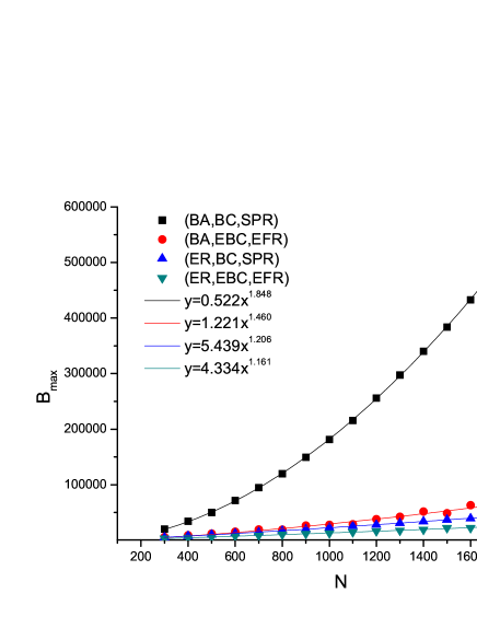
Figure 1: (Color online) Scalability of the maximal betweenness and effective betweenness for BA and ER networks. With SPR, the $Y$-axis denotes the value of maximal betweenness, and with EFR, the $Y$-axis denotes the maximal effective betweenness. The line fittings for these data are also presented.

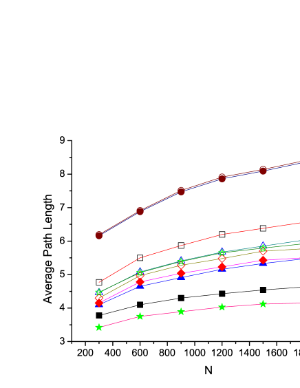
Figure 2: (Color online) Average path length for the five networks with different size under both shortest path routing and efficient routing. The filled shape represents the SPR, while the hollow shape represents the EFR.

The performance gain or tradeoff are indeed quantifiable in these four schemes. Table 5 presents the $R_{c}$ and $C_{max}$ of these four schemes. Recall that with uniform node capability scheme, $R^{\Gamma}_{c}=\frac{CN(N-1)}{B^{\Gamma}_{max}}$, so the result for (UC, SPR) and (UC, EFR) is obvious.

For $R_{c}$ in (BC, SPR), we rewrite Equation 2 as follows:

$$\begin{split}R_{c}&=min_{i}\frac{C(i)N(N-1)}{B(i)}\\ &=min_{i}\frac{B(i)/\sum_{j=1}^{N}B(j)\times 4N\times N(N-1)}{B(i)}\\ &=\frac{4N^{2}(N-1)}{\sum_{j=1}^{N}B(j)}\\ &=\frac{4N^{2}(N-1)}{N(N-1)(L_{G}+1)}\\ &=\frac{4N}{L_{G}+1}\end{split}$$ (3)

    where $L_{G}$ is the average shortest path length of $G$.

Since $\sum_{j=1}^{N}{B(j)}=N(N-1)(L_{G}+1)$, it is easy to demonstrate that $C_{max}=\frac{4B_{max}}{(N-1)(L_{G}+1)}$. Similarly, by replacing $B_{max}$ with $B^{(EFR)}_{max}$, and $L_{G}$ with $L^{(EFR)}_{G}$, we get the $R_{c}$ and $C_{max}$ for (EBC, EFR).

From Table 5, it is easy to explain the previous observations. In BA and PA networks, $B_{max}$ can be an order of magnitude larger than $B^{(EFR)}_{max}$(see Fig.1), which explains why the performance gain of $R_{c}$ is remarkable in these networks.

With (BC, SPR), $R_{c}$ is purely determined by the average path length of the given network. Since most networks have the small-world property, their $R_{c}$ values will be very large, and will not differ significantly. This property also explains the drastic difference shown by ring and lattice, since their average path lengths are $\Theta(N)$ and $\Theta(\sqrt{N})$ respectively. However, (BC, SPR) can incur high $C_{max}$ because it is proportional to the largest node betweeness, which can be very high in heterogeneous networks. Indeed, as is shown in Table 4, $C_{max}$ can differ by an order of magnitude for different networks.

For heterogenous networks, (EBC, EFR) can achieve $R_{c}$ slightly lower than the optimal one while at meantime significantly reduces $C_{max}$. This effect arises from the following facts:

$$\frac{R^{(BC,SPR)}_{c}}{R^{(EBC,EFR)}_{c}}=\frac{L^{(EFR)}_{G}+1}{L_{G}+1}$$ (4)

and

$$\frac{C^{(BC,SPR)}_{max}}{C^{(EBC,EFR)}_{max}}=\frac{L^{(EFR)}_{G}+1}{L_{G}+1}\times\frac{B_{max}}{B^{(EBC,EFR)}_{max}}$$ (5)

In most networks, $L^{(EFR)}_{G}$ is only slightly longer than $L_{G}$, as is evidenced in Fig.LABEL:cmax, so the ratio between $R^{(BC,SPR)}_{c}$ and $R^{(EBC,EFR)}_{c}$ is slightly larger than 1. However, $C^{(BC,SPR)}_{max}$ can be several times larger than $C^{(EBC,EFR)}_{max}$, mainly due to the potentially dramatic difference between $B_{max}$ and $B^{(EBC,EFR)}_{max}$. This property is the foundation of the cost-effectiveness of (EBC, EFR).

5.2 Scalability and adaptability of $R_{c}$ and $C_{max}$

One question of interest is how $R_{c}$ and $C_{max}$ scales in different settings as network size grows. Figure 3 and 4 present the $R_{c}$ and $C_{max}$ values for BA and ER networks under four different settings. It is shown that under (UC, SPR), BA network’s $R_{c}$ value remains quite stable, i.e., almost not scaling with $N$. This is because, $B_{max}$ scales super linearly with $N$, as illustrated in Fig. 1. Simulation result shows that $B_{max}\sim N^{1.848}$ in BA network, whereas in ER network, $B_{max}\sim N^{1.460}$. On the other hand, $B^{(EFR)}_{max}$ grows much slowly as network expands, $\sim N^{1.206}$ and $\sim N^{1.161}$ for BA and ER respectively. This means with (UC, SPR), BA network’s $R_{c}$ scales very slowly, while ER network’s $R_{c}$ scales much better. However, with (UC, EFR) the scalability of $R_{c}$ significantly improves for BA network. With (BC, SPR) or (EBC, EFR), the formula in Table 5 guarantees good scalability of $R_{c}$ for small-world networks.

As for $C_{max}$, with (BC, SPR), $C_{max}\propto B_{max}$, so it grows fast for BA network, and much more slowly for ER network. With (EBC, EFR), $C_{max}\propto B^{(EFR)}_{max}$, which scales much slowly in BA networks. This is evidenced in Fig.4, where $C_{max}$ grows fast with (BA, BC, SPR), but remains nearly stable for (BA, EBC, EFR) and (ER, EBC, EFR). For clarity, we do not present WS and PA in Fig. 4, but the growth trends of WS and PA are similar to ER and BA respectively.

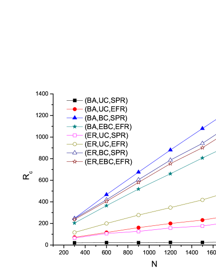
Figure 3: (Color online) Scalability of $R_{c}$ values of BA, HOT and ER under four different configurations.

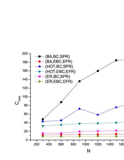
Figure 4: (Color online) Scalability of $C_{max}$ values of BA and ER under (BC,SPR) and (EBC, EFR) schemes.

6 Conclusion

In this Letter, we proposed that network designing is a multi-objective optimization designing process and involves several seemingly independent but in fact closely related aspects. We found that betweenness based capability scheme combined with shortest path routing can achieve highest network transmission capability, but this scheme also requires high cost. If the network topology is predetermined and has small-world property, then the efficient routing combined with effective betweenness based node capability scheme, abbreviated as (EBC, EFR), can achieve good balance between the network transmission capacity and designing cost in most cases, except for networks with rigid hierarchical structures such as HOT network. In addition, (EBC, EFR) also has good scalability for both $R_{c}$ and $C_{max}$. Among all networks, ER network is a markedly good candidate to achieve cost-effective designing, especially when routing algorithm and node capability scheme can not be determined beforehand.

- [1] S. P. Borgatti, Soc. Netw. 27, 55 (2005).
- [2] K. -I. Goh, B. Kahng, and D. Kim, Phys. Rev. Lett. 87, 278701 (2001).
- [3] N. Gupte and B. K. Singh, Euro. Phys. B. 50, 227 (2006).
- [4] R. Guimer, A. Z. Guilera, F. V. Redondo, A. Cabrales, and A. Arenas, Phys. Rev. Lett. 89, 328170 (2002).
- [5] H. Li and M. Maresca, IEEE. Trans. Computers 38, 1345 (1989).
- [6] G. Q. Zhang, D. Wang, and G. J. Li, Phys. Rev. E 71, 017101 (2007).
- [7] G. Yan, T. Zhou, B. Hu, Z. Q. Fu, and B. H. Wang, Phys. Rev. E 73, 046108 (2006).
- [8] L. Zhao, Y. C. Lai, K. Park, and N. Ye, Phys. Rev. E 71, 026125 (2005).
- [9] B. Danila, Y. Yu, J. A. Marsh, and K. E. Bassler, Phys. Rev. E 74, 046106 (2006).
- [10] G. Q. Zhang, S. Zhou, G. Yan, D. Wang, and G. Q. Zhang, arXiv:0910.2285 (2009).
- [11] L. Li, D. Alderson, W. Willinger, J. Doyle, Proc. ACM SIGCOMM 2004 (ACM Press, Oregon, 2004).
- [12] A. Arenas, A. Díaz-Guilera, and R. Guimerà, Phys. Rev. Lett. 86, 3196 (2001).
- [13] L. C. Freeman, Soc. Netw. 1, 215 (1979).
- [14] G. Q. Zhang, B. Yuan, and G. Q. Zhang, Proc. IEEE Next Generation Internet Networks (IEEE Press, Norway, 2007).
- [15] P. Erdös and A. Rényi, Publ. Math. Debrecen 6, 290 (1959).
- [16] B. Bollobas.: Random Grpahs (Cambridge University Press) (1985).
- [17] D. J. Watts and S. H. Strogatz, Nature 393, 440 (1998).
- [18] A. L. Barabsi and R. Albert, Science 286, 509 (1999).