A model for signal transduction during quorum sensing in Vibrio harveyi

Abstract

We present a framework for analyzing luminescence regulation during quorum sensing in the bioluminescent bacterium Vibrio harveyi. Using a simplified model for signal transduction in the quorum sensing pathway, we identify key dimensionless parameters that control the system’s response. These parameters are estimated using experimental data on luminescence phenotypes for different mutant strains. The corresponding model predictions are consistent with results from other experiments which did not serve as inputs for determining model parameters. Furthermore, the proposed framework leads to novel testable predictions for luminescence phenotypes and for responses of the network to different perturbations.

1 Introduction

Bacterial survival critically depends on regulatory networks which integrate multiple inputs to implement important cellular decisions. A prominent example is the global regulatory network involved in “quorum sensing”, commonly defined as the regulation of gene expression in response to cell density. During the process of quorum sensing (QS), bacteria produce, secrete and detect signaling molecules called autoinducers (Miller and Bassler 2001; Waters and Bassler 2005; Bassler and Losick 2006). These signals are then processed by the QS pathway to regulate critical bacterial processes such as biofilm formation and virulence. The observation that quorum sensing is linked to both biofilm formation and virulence factor production suggests that many virulent bacteria can be rendered nonpathogenic by the inhibition of their QS pathways (Bjarnsholt and Givskov 2007). Quantitative modeling of the QS pathway can thus provide useful inputs for treating many common and damaging bacterial infections.

One of the most studied model organisms for QS based regulation is the bioluminescent marine bacterium Vibrio harveyi (Nealson et al., 1970). Experimental studies have led to a detailed characterization of regulatory elements in the pathway (Henke and Bassler 2004; Mok et al., 2003; Timmen et al., 2006; Waters and Bassler 2006; Tu and Bassler 2007). The network (see Fig. 1) includes multiple autoinducers and corresponding sensor proteins which act together to control the phosphorylation of the response regulator protein LuxO. The phosphorylated form of LuxO (LuxO-P) activates the production of multiple small RNA (sRNA)s which in turn post-transcriptionally repress the QS master regulatory protein LuxR. At low cell density, the sRNAs are activated and act to effectively repress LuxR expression. In contrast, sRNA production is significantly reduced at high cell density, thereby giving rise to increased levels of LuxR which leads to the activation of luminescence genes. The corresponding luminescence output per cell profile (i.e., colony luminescence/cell output as a function of cell density) is frequently used as a reporter to characterize the state of the QS pathway.

Recent experiments (Henke and Bassler 2004) have analyzed the effects of mutagenesis of different pathway components on the corresponding luminescence profile in V. harveyi. It was observed that there are distinct luminescence profiles as the network is perturbed corresponding to different pathway mutants. The changes in the luminescence profile were used to infer pathway characteristics such as relative kinase strengths for the different sensors. Given the complexity of the network which involves integration of multiple inputs, it would be desirable to develop a quantitative framework for inferring pathway characteristics based on network perturbations. The corresponding quantitative model can then be used to make testable predictions for future experiments as well as to further analyze existing experimental data. The aim of this work is to develop such a minimal model for the QS pathway in V. harveyi.

The starting point of our analysis is the observation that luminescence/cell output is controlled by the degree of phosphorylation of the response regulator LuxO. We thus develop a simplified model which connects external autoinducer concentrations to the degree of phosphorylation of LuxO for the wild type (WT) strain and for different mutants. Our analysis identifies key dimensionless parameters which control the system response and which can be determined using the experimental results for luminescence phenotypes. Determination of the effective parameters, in turn, leads to predictions for the systems response to a broader range of perturbations, i.e., perturbations distinct from those used to infer the effective parameters. The corresponding analysis sheds light on previously obtained experimental results and also gives rise to testable predictions for future experiments.

The rest of the paper is organized as follows. In Section 2 we give an overview of the QS network in V. harveyi. We then develop a minimal model of the QS pathway and define key dimensionless parameters which control the network response characteristics. In Section 3, we connect our model to experimental data on different luminescence curves and thereby determine model parameters. In Section 4, we discuss experimentally testable predictions based on the model and conclude with a summary.

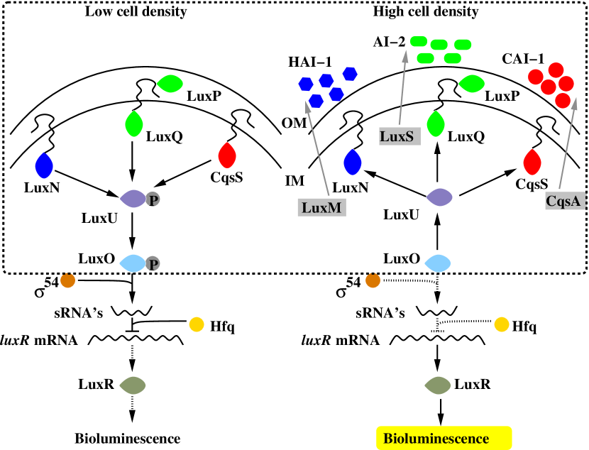
Figure 1: (color online) Schematic representation of quorum sensing network in Vibrio harveyi at high and low cell densities. The dotted rectangle is the input module which controls phosphorylation of LuxO in response to external autoinducer concentrations. Solid line, active path; Dotted line, inactive path; IM, inner membrane; OM, outer membrane.

2 Overview and Model

The QS network in V. harveyi is shown in Fig. 1. The key upstream components of the pathway are the three sensors, LuxN, LuxPQ and CqsS_Vh and the corresponding autoinducer synthases, LuxM, LuxS, and CqsA_Vh which are responsible for producing the three autoinducers: H-AI1, AI-2, and CAI-1, respectively. The binding of a single autoinducer to a sensor is highly specific, i.e., HAI-1 binds only to LuxN, AI-2 binds to LuxPQ only, and CAI-1 binds specifically to CqsS_Vh (see Fig. 1). The overall network is conveniently described in terms of functional modules. The first (input) module includes interactions between autoinducers ([AI_i] ($i=1,2,3$)) and the corresponding sensor proteins which, through a phosphorelay mechanism, determine the overall phosphorylation state of a $\sigma^{\mathrm{5}4}$-dependent response regulator LuxO.

The second module focuses on the regulated production of sRNAs (dependent on the phosphorylation state of LuxO) and the interaction between the sRNAs and the master regulator protein, LuxR. The interactions between small RNAs and their regulated targets have been modeled in several recent studies which shed light on how target protein expression is controlled by small RNA-mediated regulation (Lenz et al., 2004; Levine et al., 2007; Levine and Hwa 2008; Mehta et al., 2008; Mitarai et al., 2007). In V. harveyi, LuxR serves as the target protein whose expression is controlled by the small RNAs in combination with the RNA-binding protein Hfq. The resulting concentration of LuxR determines the level of activation or repression of a multitude of genes including the genes involved in bioluminescence (Waters and Bassler 2006). The corresponding change in the luminescence/cell output determines the luminescence profile which is frequently used to infer network characteristics such as relative rates of kinase/phosphotase activities by the sensor proteins (Henke and Bassler 2004).

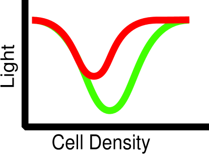
Figure 2: (color online) Schematic representation of typical luminescence curves from experiment. The green curve represents the response from a wild type (WT) colony. The turnaround point in the curve corresponds to cell density necessary for the activation of the genes responsible for luminescence output per cell. The red curve represents the luminescence/cell curve for a mutant strain that is able to achieve the same activation at a lower cell density.

A schematic representation of typical luminescence/cell curves is shown in Fig. 2. Since the starting point is obtained by the dilution of cells in the high density limit, the luminescence output per cell is maximal at the initial time points. The luminescence output per cell then declines steadily with increasing cell density, since luminescence genes are no longer activated in the cells. At a specific cell density, the luminescence curve starts to rise again signalling the start of de novo luminescence gene activation by cells in the growing colony. The cell density necessary for activation can vary from the WT and mutant strains resulting in different luminescence phenotypes (see Fig. 2).

Current data indicates that increasing cell density leads to increasing dephosphorylation of LuxO leading to lower production rates for the sRNAs. Correspondingly, the turnaround point in the luminescence curves corresponds to unphosphorylated LuxO reaching a critical level above which sRNA production is not effective at repressing LuxR levels below the threshold for observable luminescence activation in the population of cells. Thus, understanding how external signals (i.e., AI concentrations as a function of cell density) are translated into the degree of LuxO phosphorylation (i.e., the input module) is critical for analyzing luminescence profiles. Furthermore, pathway mutants which function upstream of LuxO are not known to have any direct effects on sRNA production or LuxR levels, apart from the indirect effects mediated by LuxO. Therefore we expect that the critical level of LuxO phosphorylation corresponding to the turnaround in the luminescence profile is the same for all mutants. The observation that the luminescence profiles are different for different pathway mutants indicates different functional relations between external AI concentrations and LuxO phosphorylation levels for the different mutants. In the following, we derive a simple model which connects cell density to LuxO phosphorylation and uses information from luminescence profiles of different mutants to infer system parameters.

The sensor proteins in the QS pathway can be modeled as two state systems (Neiditch et al., 2006; Swem et al., 2008). We consider a further simplification which takes the sensors to be existing either in the kinase mode, $S_{ki}$, or in the phosphatase mode, $S_{pi}$ (where $i=1,2,3$ corresponds to the distinct sensor proteins in V. harveyi). In the kinase mode, the sensors can autophosphorylate and then transfer the phosphate group to the downstream protein LuxU, whereas in the phosphatase mode the phosphate flow is reversed. Experiments indicate that at low cell density (corresponding to low autoinducer concentrations) the sensors are primarily in the kinase mode, whereas at high cell density (corresponding to high autoinducer concentrations), the sensors are primarily in the phosphatase mode. Correspondingly, we consider a simplified model wherein the free sensor corresponds to the kinase mode, whereas binding of autoinducer results in a transition to the phosphatase mode.

At a given cell density, the external autoinducer concentrations will be proportional to the colony forming units $N$. Since the time scale for changes in $N$ (i.e., the doubling time) is large compared to the time scales for binding/unbinding of ligands and subsequent phophorylation/dephosphorylation, the corresponding reactions can be considered in steady state for a given $N$. Furthermore, since the typical number of sensor proteins of each type is large, the concentration of sensors of type $i$ is well approximated by the mean value $[S_{i}]=c_{i}[S_{0}]$ (where $[S_{0}]$ is some reference concentration). At a given cell density, external AI concentrations determine the fraction of the receptors which exist in either the kinase or phosphatase mode. For the simplest case of autoinducers binding to their cognate sensors, we have the kinetic scheme:

$$S_{ki}+AI_{i}\binrel@{\binrel@{\rightleftharpoons}\binrel@@{\mathop{\kern 0.0pt\rightleftharpoons}\limits_{k_{-i}}}}\binrel@@{\mathop{\kern 0.0pt\binrel@{\rightleftharpoons}\binrel@@{\mathop{\kern 0.0pt\rightleftharpoons}\limits_{k_{-i}}}}\limits^{k_{i}}}S_{pi},$$ (1)

from which the mean steady state concentrations of the sensors in either the kinase or phosphatase mode can be obtained. More generally, to account for cooperative effects in binding, we take the kinase/phosphatase fractions to be:

$$[S_{ki}]=(1-g_{i})c_{i}[S_{0}]\;{\rm and}\;[S_{pi}]=g_{i}c_{i}[S_{0}],$$ (2)

where

$$[S_{ki}]+[S_{pi}]=c_{i}[S_{0}],g_{i}=a_{i}^{n}/(1+a_{i}^{n}),a_{i}=[AI_{i}]/\kappa_{i}.$$ (3)

and $\kappa_{i}=k_{-i}/k_{i}$.

Equation (2), with Hill coefficient $n=1$, corresponds to the steady state fractions for equation (1), higher $n$ values correspond to sharper switching from kinase to phosphatase mode which mimics cooperative effects in binding. Finally, since the concentration of the $i$-th autoinducer, [$AI_{i}$], is proportional to the colony forming units (CFU), $N$, i.e. $[AI_{i}]=\nu_{i}N$; we renormalize the binding constant $\kappa_{i}$ to define the scaled effective parameter $\bar{\kappa}_{i}=\kappa_{i}/\nu_{i}$.

Typically in bacterial signal transduction, the sensor proteins in the kinase/phosphatase modes serve as enzymes which transfer the phosphate group to/from a response regulator protein or a phosphorelay protein (Appleby 1996; Hoch 2000; Stock et al., 2000; Laub and Goulian 2007). In V. harveyi, this step involves phosphotransfer to the phosphorelay protein LuxU ($U$). Phosphorylated LuxU ($U_{P}$) can then transfer the phosphate group to the response regulator LuxO ($O$); similarly, unphosphorylated LuxU serves as a receiver for removing the phosphate group from phosphorylated LuxO ($O_{P}$) . We represent these processes by the following equations:

$$S_{ki}+U \binrel@{\rightarrow}\binrel@@{\mathop{\kern 0.0pt\rightarrow}\limits^{k_{ki}}} S_{ki}+U_{P},$$ (4a)

$$S_{pi}+U_{P} \binrel@{\rightarrow}\binrel@@{\mathop{\kern 0.0pt\rightarrow}\limits^{k_{pi}}} S_{pi}+U,$$ (4b)

$$U_{P}+O \binrel@{\binrel@{\rightleftharpoons}\binrel@@{\mathop{\kern 0.0pt\rightleftharpoons}\limits_{k_{b}}}}\binrel@@{\mathop{\kern 0.0pt\binrel@{\rightleftharpoons}\binrel@@{\mathop{\kern 0.0pt\rightleftharpoons}\limits_{k_{b}}}}\limits^{k_{f}}} U+O_{P}.$$ (4c)

For the above kinetic equations, it is convenient to define key dimensionless parameters of the model as follows

$$\alpha_{ri}=c_{i}k_{ki}/k_{kr},~{}\beta_{i}=(k_{f}/k_{b})(k_{ki}/k_{pi}).$$ (4e)

The parameter $\alpha_{ri}$ is a measure of the relative kinase strength of $i$-th sensor with respect to the $r$-th sensor (scaled by the mean concentrations of the two sensors), e.g., $\alpha_{12}$ is the relative kinase strength of sensor 2 with respect to sensor 1. Another set of key parameters is the ratio of the scaled kinase to phosphatase rates, $\beta_{i}$, of the $i$-th sensor. Using these dimensionless parameters, we then solve the rate equations (4a-4c) at steady state to derive the following expression for the fraction of unphosphorylated LuxO at steady state, $f_{\rm LuxO}=[O]/[O]_{0}$ (with $[O]_{0}$ being the total LuxO concentration)

$$f_{\rm LuxO}=\frac{\sum_{i}\alpha_{ri}(g_{i}/\beta_{i})}{\sum_{i}\alpha_{ri}(1-g_{i})+\sum_{i}\alpha_{ri}(g_{i}/\beta_{i})}.$$ (4f)

3 Connection to experimental data

We now connect the model for LuxO phosphorylation developed in the previous section to experimental luminescence curves. Recall that the typical luminescence profile shows a well defined switching point which signals observable de novo production of luminescence by the population of cells. As argued earlier, this corresponds to a critical value for the concentration of unphosphorylated LuxO. Let us denote this critical fraction of unphosphorylated LuxO by $f^{c}$ and the corresponding value of the colony forming units by $N^{c}$. At $f_{\rm LuxO}=f^{c}$, for the WT luminescence curve we have the following relation (4f):

$$\sum_{i}\alpha_{ri}(1-g_{i})=\left(\frac{1-f^{c}}{f^{c}}\right)\sum_{i}\alpha_{ri}(g_{i}/\beta_{i}),$$ (4g)

where the factors $g_{i}$ are evaluated at $N=N^{c}$. Since $N^{c}$ is known from experiments corresponding to the WT luminescence curve, the above equation can be regarded as a constraint on the dimensionless parameters.

We now consider the corresponding equations for luminescence phenotypes of the mutant strains. Current knowledge of the QS network in V. harveyi indicates that pathway proteins functioning upstream of LuxO primarily control LuxO phosphorylation levels and have no direct interactions with the qrr sRNAs or the master regulator LuxR. This suggests that for each mutant the degree of LuxO phosphorylation needed to activate luminescence is the same (i.e., $f^{c}$ is the same) since upstream proteins affect LuxR only via LuxO-P levels. The observation that the luminescence profiles are distinct for different pathway mutants is a consequence of the altered functional relationship between LuxO phosphorylation levels and external autoinducer concentrations for the mutants. Given the defined roles of the pathway proteins, these altered functional relationships can readily be derived within our model for all the mutants. For example, equation (4g) for the single sensor mutant $cqsS_{Vh}$ (i.e. the strain with a deletion for the gene $cqsS_{Vh}$) takes the form:

$$(1-g_{1})+\alpha_{12}(1-g_{2})=\left(\frac{1-f^{c}}{f^{c}}\right)\left[\frac{g_{1}}{\beta_{1}}+\alpha_{12}\frac{g_{2}}{\beta_{2}}\right].$$

Note that the quantity $(1-f^{c})/f^{c}$ can be absorbed into the scaled kinase to phosphatase ratios $\beta_{1}$ and $\beta_{2}$. This is equivalent to setting $f^{c}=1/2$ in the above equation, and since $f^{c}$ is the same for all pathway mutants, a similar rescaling can be done for the functional relationships for all the mutants. The corresponding equations are presented in the Appendix. In the following, we show how these equations can be used along with WT and mutant luminescence phenotypes to determine effective system parameters and to make testable predictions.

From the work of Henke and Bassler (2004), the critical threshold in colony forming units ($N^{c}$) can be estimated for a range of pathway mutants. The different mutant strains studied were i) $luxN$, ii) $luxQ$, iii) $cqsS_{Vh}$, iv) $luxN\ luxQ$, v) $luxN\ cqsS_{Vh}$, and vi) $luxQ\ cqsS_{Vh}$. To connect the sensors of V. harveyi with our model, we designate sensors LuxN, LuxQ, and CqsS_Vh as $1$, $2$, and $3$, respectively. The ordering of the CFU/volume for the different strains at their critical threshold shows the following hierarchy (Henke and Bassler 2004):

$$N_{12}^{c}\ll N_{2}^{c}\sim N_{23}^{c}<N_{wt}^{c}<N_{3}^{c}<N_{1}^{c}\sim N_{13}^{c},$$ (4h)

where $N_{12}^{c}$ is the number of colony forming units for mutant strain $luxN\ luxQ$ at which $f_{\rm LuxO}=f^{c}$ and so on. Although the values $N_{2}^{c}$, $N_{23}^{c}$ and $N_{1}^{c}$, $N_{13}^{c}$ appear to be indistinguishable based on available experimental data, based on the model developed we expect a small difference in the threshold values. For example, the difference between the luxN strain and luxN cqsS_Vh strain is that CqsS_Vh is active as phosphatase in the luxN mutant (close to the switching threshold). This implies that the switching in the luminescence phenotype should occur at a lower $N^{c}$ value for the luxN cqsS_Vh strain i.e., $N_{1}^{c}<N_{13}^{c}$. Since CqsS_Vh has weak effect on the luminescence phenotype, the switching values are indistinguishable experimentally. However to develop a consistent model, we have to impose a small difference between the switching values based on the constraint $N_{1}^{c}<N_{13}^{c}$ (and similarly for $N_{2}^{c}$ and $N_{23}^{c}$).

Based on the above reasoning, we initially considered a $\sim$10% difference between $N_{2}^{c}$, $N_{23}^{c}$ and $N_{1}^{c}$, $N_{13}^{c}$. Accordingly, the values for critical thresholds (switching values, in the units of CFU/volume) used as initial inputs were

$$N_{12}^{c}\sim 1\times 10^{5},N_{2}^{c}\sim 14\times 10^{5},N_{23}^{c}\sim 15\times 10^{5},N_{wt}^{c}\sim 40\times 10^{5},$$

$$N_{3}^{c}\sim 70\times 10^{5},N_{13}^{c}\sim 110\times 10^{5},N_{1}^{c}\sim 100\times 10^{5}.$$

From the discussion of the previous section, we have seen that the input module provides us eight key parameters: two relative kinase strengths ($\alpha_{12}$ and $\alpha_{13}$), three scaled kinase to phosphatase ratios ($\beta_{1}$, $\beta_{2}$, and $\beta_{3}$) and three effective binding constants ($\bar{\kappa}_{1}$, $\bar{\kappa}_{2}$, and $\bar{\kappa}_{3}$). Given that we have experimental data for threshold cell densities for seven strains, this indicates that if one of the parameters is fixed, the other parameters can potentially be determined by solving the corresponding threshold equations (see Appendix). Since previous work indicated that the effect of CqsS_Vh on luminescence phenotypes is minimal, we initially fixed the parameter $\alpha_{13}$ (the relative kinase strength of sensor 3 (CqsS_Vh) with respect to sensor 1 (LuxN)) to 0.001.. We then proceeded to determine the effective model parameters by solving the threshold equations using the above experimental inputs for switching cell densities. We also checked the stability of the solutions to the above equations based on small perturbations to the input parameters (data not shown). We found that the solutions are stable with respect to perturbations that maintain the initial $\sim$10% difference between $N_{2}^{c}$, $N_{23}^{c}$ and $N_{1}^{c}$, $N_{13}^{c}$. However the solutions are sensitive to changes in the parameters controlling the small differences in $N_{c}$ values. Since experiments cannot guide us in determining the precise value of these differences, the values of $N_{2}^{c}$ and $N_{1}^{c}$ do not serve as useful inputs in determining model parameters. Thus additional experimental data is needed to determine model parameters as outlined below.

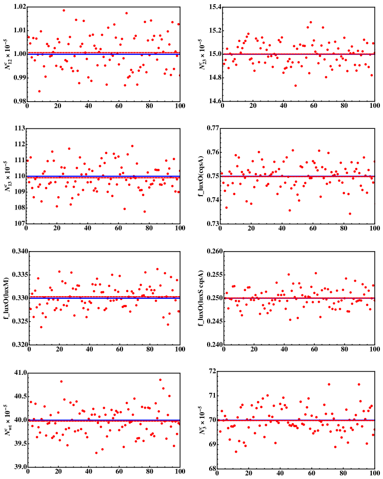
Figure 4: (color online) Results of sensitivity analysis for the input base values The blue line represents the unperturbed data and the red dashed line is the mean of the 100 perturbed data points represented by scattered red points.

The luminescence data at high cell densities (hcd) for different sensor mutants from the work of Henke and Bassler (2004) (see Fig. 4A) provides an indirect means of estimating model parameters. The basic experimental observations can be summarized as follows: while the WT strain shows a bright phenotype at hcd, the $luxS$ strain has a dim phenotype and the $luxM$ strain has low levels of luminescence and is classified as being dark. Furthermore the $cqsS_{Vh}$ strain has a luminescence output that is intermediate between WT and $luxS$ and the $cqsA_{Vh}\ luxS$ double mutant is dark and produces significantly less luminescence than a $luxM$ strain. Given our definitions of model parameters, $f_{\rm LuxO}=1/2$ corresponds to value at which observable luminescence/cell is produced. Higher values of $f_{\rm LuxO}$ will correspond to brighter luminescence phenotypes, whereas a dark luminescence phenotype implies $f_{\rm LuxO}<1/2$. Thus we expect that, at hcd, we have $f_{\rm LuxO}$ for $luxS$ mutants to be around 0.5 (given the dim luminescence phenotype) and $f_{\rm LuxO}$ for the $cqsS_{Vh}$ strain to be significantly greater than the corresponding value for the $luxS$ strain but significantly lower than 1 (the value for the WT strain). Based on these constraints, we set the $f_{\rm LuxO}$ values for 3 synthase mutant strains at hcd as follows: $f_{\rm LuxO}^{cqsA}=3/4$, $f_{\rm LuxO}^{luxm}=1/3$ and $f_{\rm LuxO}^{luxS\ cqsA}=1/4$. In combination with the expression derived for $f_{\rm LuxO}$ (equation (4f)), these equations can be used, along with luminescence switching cell density equations, to determine model parameters (see Appendix).

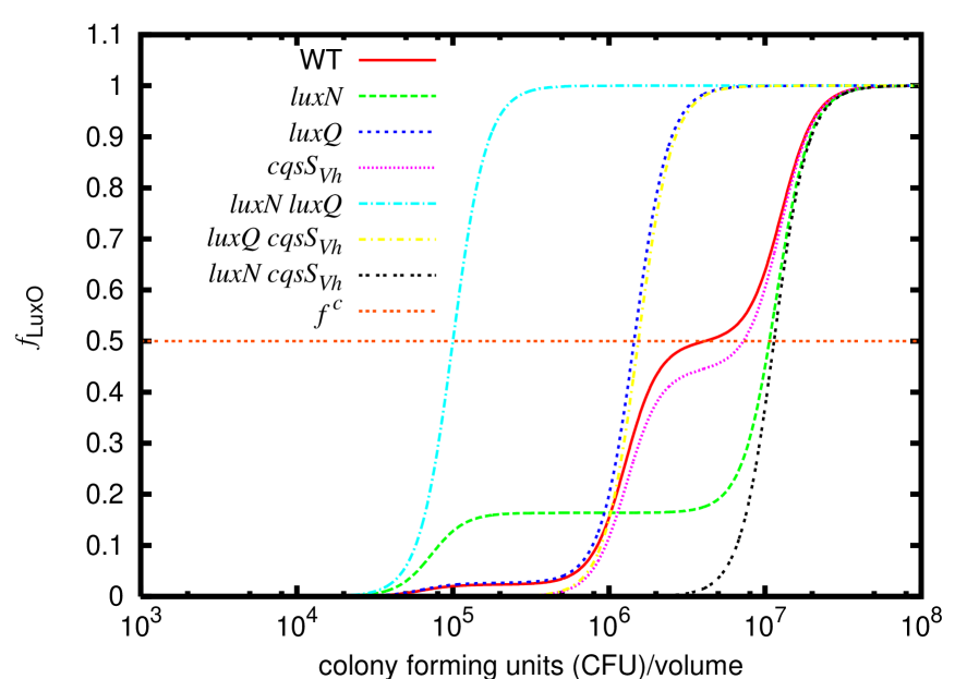
Figure 3: (color online) Profile of $f_{\rm LuxO}$ as a function of colony forming units (CFU)/volume for wild type (WT) and different sensor mutant phenotypes. The cell density at which $f_{\rm LuxO}=f^{c}$ corresponds to the turnaround point in the experimental luminescence curves.

First, considering equation (4g) for the double sensor mutants, we have the relation between the three $\beta$-s and three $\bar{\kappa}$-s,

$$N_{23}^{c}=\bar{\kappa}_{1}\beta_{1}^{1/n},N_{13}^{c}=\bar{\kappa}_{2}\beta_{2}^{1/n},N_{12}^{c}=\bar{\kappa}_{3}\beta_{3}^{1/n}.$$ (4i)

Also from equation (4g), we have the expressions for the wild type and one single sensor mutant ($cqsS_{Vh}$) with five unknown parameters: three kinase to phosphatase ratios ($\beta_{1}$, $\beta_{2}$ and $\beta_{3}$) and two relative kinase strength ($\alpha_{12}$ and $\alpha_{13}$) (Note that we are now considering $\alpha_{13}$ to be variable). Using $f_{\rm LuxO}=f^{c}=1/2$, the switching values for WT and $cqsS_{Vh}$, ($N_{wt}^{c}$ and $N_{3}^{c}$) and the $f_{\rm LuxO}$ for three synthase mutants at hcd we solve the five equations to determine the five unknown parameters. The corresponding values for the key parameters of the model are: $\alpha_{12}\sim 0.14$, $\alpha_{13}\sim 0.19$, $\beta_{1}\sim 8.99$, $\beta_{2}\sim 0.29$ and $\beta_{3}\sim 7.14$, for the Hill coefficient $n=4$. We note that there are two sets of solutions obtained using the above approach, however only one of these corresponds to the experimentally observed hierarchy of switching cell densities (4h). Furthermore no solutions were obtained for $n\leqslant 2$. For $n=3$, the equations can be solved and yield parameters that are close to the those inferred for $n=4$. However the $n=4$ results are more consistent with the experimental observation that the switching cell densities are experimentally indistinguishable for $N_{1}^{c}$ and $N_{13}^{c}$ (similarly for $N_{2}^{c}$ and $N_{23}^{c}$). The high value of $n=4$ suggests that there might be cooperative effects in the switch from the kinase to phosphatase mode for the sensors. Now using these values for the effective parameters, we calculate the values of $f_{\rm LuxO}$ as a function of CFU/volume (see Fig. 3) for the WT and different sensor mutant phenotypes of V. harveyi. Since the effective parameters are determined, we can now use our model to generate similar curves and make predictions for mutants that have not yet been studied experimentally. We have checked the stability of the obtained solutions with respect to small changes in the input values (see Appendix). We have also considered larger changes in the input $f_{\rm LuxO}$ values consistent with the constraints noted earlier. While the precise values of the effective model parameters do change as the inputs are varied, there are several robust predictions that can be made. These are discussed further in the concluding section.

4 Conclusion and outlook

The preceding analysis helps determine the parameters in our minimal model. While these parameters cannot directly be compared to experiments, they can lead to several predictions which are testable experimentally. In the following, we outline some of the key predictions based on our analysis.

1) The parameter $\beta_{i}$ is a measure of the relative kinase to phosphatase rates for the $i$-th sensor. Based on the values determined, the following ordering is predicted for the relative kinase to phosphatase rates of the three sensors LuxN $>$ CqsS_Vh $>$LuxQ. LuxN is predicted to be the strongest kinase which is consistent with results from previous experiments showing that LuxN has a greater effect on LuxO phosphorylation than LuxQ (Freeman et al., 2000). Furthermore, it is interesting to note that recent experiments have demonstrated high kinase to phosphatase rates for the sensor LuxN (Timmen et al., 2006). While the corresponding value estimated by our model ($\beta_{1}\sim 9$) cannot directly be compared to experiments since it involves additional parameters, the ratio $\beta_{i}/\beta_{j}$ $(i\neq j)$ should correspond to experimental estimation of the ratio of kinase to phosphatase rates of two sensors. From our model we consistently find that $\beta_{2}/\beta_{1}\ll 1$ and $\beta_{2}/\beta_{3}\ll 1$ indicating the the effective kinase to phosphatase activity ratio for LuxQ is much lower than the other two sensors. Note that this prediction differs significantly from the previous characterization (Henke and Bassler 2004) that kinase to phosphatase activity ratio for LuxQ is greater than that of CqsS_Vh. It would thus be of interest to carry out experiments to measure relative kinase to phosphatase rates for the sensors LuxQ and CqsS_Vh to see if the predictions are borne out.

2) Experiments with mutant strains (besides those used as inputs to our model) indicate that at high cell densities, the luminescence phenotypes can be broadly categorized into 3 types: dark, dim and bright. Since $f^{c}=1/2$ is the threshold for luminescence activation in our model, we take these categories to correspond to the following: dark ($0\leqslant f_{\rm LuxO}<0.4$), dim ($0.4<f_{\rm LuxO}<0.6$) and bright ($0.6<f_{\rm LuxO}\leqslant 1.0$). Using these criteria, we can now predict the luminescence phenotypes at high cell density for other pathway mutants (i.e. those not included in the experimental inputs used to determine model parameters). The corresponding results are listed in Table 1. We note that all mutant strains with LuxM deleted ($luxM$) are dark. This is consistent with previous experimental results (Freeman and Bassler 1999). Other interesting predictions are
i) While $cqsA_{Vh}\ luxN$ is bright (comparable to $cqsA_{Vh}$) at hcd, the strain $cqsA_{Vh}\ luxQ$ is predicted to be dark;
ii) $luxS$ is brighter than $luxM$ at hcd , however $cqsA_{Vh}\ luxS$ is predicted to be darker than $cqsA_{Vh}\ luxM$ (note that this is consistent with the observations in Henke and Bassler (2004)).

Table 1: Predictions for luminescence output per cell of different synthase mutants and mixed sensor-synthase mutants.

• Phenotype	Mutant
  dark	$luxM$, $luxM\ luxS$, $luxS\ cqsA_{Vh}$, $luxM\ cqsA_{Vh}$,
  	$luxN\ luxS$, $luxQ\ luxM$, $luxQ\ cqsA_{Vh}$, $cqsS_{Vh}\ luxM$
  dim	$luxS$, $cqsS_{Vh}\ luxS$
  bright	$cqsA_{Vh}$, $luxN\ cqsA_{Vh}$

It should be noted that the results presented in Fig. 3 are just for sensor mutants whereas Table 1 is for synthase mutants and mixed sensor-synthase mutants. For the different mutants given in Table 1, the maximal value of the $f_{\rm LuxO}$ curve differs from 1 and stays within the defined range (according to the broad categories discussed in the paper) even at the hcd in contrast to the behavior shown in Fig. 3 for the sensor mutants.

3) To figure out the values of the effective parameters of the model, we have used the switching value ($N^{c}$) of WT, $cqsS_{Vh}$ and double sensor mutants from the experiment (Henke and Bassler 2004). With these derived values of the effective parameters, we can now predict the switching values of the other two bright sensor mutant strains ($luxN$ and $luxQ$) at hcd (in the units of CFU/volume),

$$N_{1}^{c}\sim 100\times 10^{5},N_{2}^{c}\sim 14\times 10^{5}.$$

It is interesting to note that the above switching values are in good agreement with the observation that $N_{1}^{c}$ is experimentally indistinguishable from $N_{13}^{c}$ and $N_{2}^{c}$ is experimentally indistinguishable from $N_{23}^{c}$ (see Fig. 3). In addition, the effective parameter set predicts the switching values ($N^{c}$, in units of CFU/volume) for the two bright mutant strains $cqsA_{Vh}$ and $luxN\ cqsA_{Vh}$ mentioned in Table 1 as $\sim 130\times 10^{5}$ and $\sim 156\times 10^{5}$, respectively.

4) Recent experiments have probed the response of the QS pathway to externally controlled autoinducer concentrations (Mok et al., 2003). In these experiments, the autoinducer production is switched off by deleting the corresponding synthases and then autoinducers are added back exogenously in controlled amounts. In our model this behavior can be mimicked by controlling the quantity $g_{i}$ in equation (3). For each synthase mutation the autoinducer production is switched off so that $g_{i}=0$ as $AI_{i}=0$ ($i=1,2,3$). As autoinducers are added to the network from outside, the quantity $g_{i}$ grows and tends to one as $AI_{i}\rightarrow\infty$. For this setup, our analysis indicates a situation wherein the sensor CqsS_Vh plays an important role in regulating the response which is contrary to what is normally assumed. Consider the situation for which all the autoinducer synthases have been deleted and subsequently saturating amounts of $AI_{1}$ are added. In this case, we predict a significant difference between the luminescence output per cell for the two cases corresponding to i) low external $AI_{3}$ concentrations and (ii) high external $AI_{3}$ concentrations. The difference between these two cases is that the sensor CqsS_Vh is primarily in kinase mode for case (i) and in phosphatase mode for case (ii). Our analysis thus suggests a testable prediction for an experimentally realizable situation wherein signaling through CqsS_Vh significantly changes the output from the QS pathway.

5) Finally, we examine predictions from our model for the expression of genes that are also controlled by $f_{\rm LuxO}$ through LuxR but are not directly related to luminescence/cell. Waters and Bassler (2006) studied several genes regulated by LuxR and classified them into different categories based on the activation/repression induced by the presence of high concentrations of either AI₁ or AI₂ or both. We will focus on the category of genes (labeled “class 3” genes) which are defined as genes that show an equally notable change in expression when either AI₁ and/or AI₂ are present in high concentrations. Within our model, we can calculate the the values of $f_{\rm LuxO}$ for the 3 cases : (i) High concentration of AI₁ only, (ii) high concentration of AI₂ only and (iii) high concentration of both AI₁ and AI₂. Out of these the lowest value of $f_{\rm LuxO}$ corresponds to case (ii) i.e., high concentration of AI₂ only. Since class 3 genes are fully activated/repressed when high concentrations of AI₂ only are present, it follows that the $f^{c}$ for all genes in this category must be lesser than the value of $f_{\rm LuxO}$ when only AI₂ levels are high ($f_{\rm LuxO}=0.33$). (Note that we have assumed that AI₃ levels are at high concentrations in the above experiments since they are at high cell densities). This observation indicates that an upper bound for activation/repression of class 3 genes corresponds to $f^{c}=0.33$. Using this, the following testable predictions can be made

• The synthase mutant $luxM$ can fully activate/repress class 3 genes at high cell density. Note that luminescence genes, in contrast, are not activated at high cell density in a $luxM$ mutant.

• Similarly, the sensor-synthase mutants $luxM\ cqsS_{Vh}$ and $luxQ\ cqsA_{Vh}$ cannot activate luminescence genes at high cell density whereas they are predicted to fully activate/repress all class 3 genes at high cell density .

The minimal model presented in this work can be generalized further as more experimental data becomes available. An important generalization would be to relax some of the assumptions made by considering a two-state model (Swem et al., 2008) which incorporates non-zero phosphatase activity in the on (free) state and nonzero kinase activity in the off (bound) state. We note that this will add several additional parameters to our current model. With additional experimental data, the generalized model could be used to estimate the expanded set of effective parameters. While the effective parameters so determined are likely to be different from the values determined using the minimal model, the framework connecting the model parameters to experimental data will essentially be the same.

In summary, we have proposed a minimal model to study the quorum sensing network in V. harveyi. Using experimental data for luminescence phenotypes of WT and different mutant strains, we provide a framework to estimate the effective dimensionless parameters of the model. Correspondingly, the model can be used to predict the luminescence phenotypes of other pathway mutants which have not been experimentally studied to date. The proposed framework captures the key features of the signal transduction in V. harveyi and can contribute to guiding and interpreting experimental efforts analyzing the QS pathway in the Vibrios.

Appendix

For the relative kinase strength ($\alpha_{ri}=c_{i}k_{ki}/k_{kr}$ for $i=1,2,3$) of the sensors, we generally use the kinase strength of LuxN, i.e., $k_{k1}(r=1)$, as the reference kinase. Now using equation (4g) we explicitly write the functional relation for WT strain evaluated at $N=N^{c}_{wt}$ for $f_{\rm LuxO}=f^{c}$:

$$(1-g_{1})+\alpha_{12}(1-g_{2})+\alpha_{13}(1-g_{3})=\left(\frac{1-f^{c}}{f^{c}}\right)\left[\frac{g_{1}}{\beta_{1}}+\alpha_{12}\frac{g_{2}}{\beta_{2}}+\alpha_{13}\frac{g_{3}}{\beta_{3}}\right].$$ (4j)

Similarly for $luxN$ mutants we use kinase strength of LuxQ, i.e., $k_{k2}(r=2)$, as the reference kinase whereas for $luxQ$ and $cqsS_{Vh}$ we use kinase strength of LuxN as the reference kinase as in WT. Thus the functional relations for the single sensor mutants $luxN$, $luxQ$ and $cqsS_{Vh}$ evaluated at $N^{c}_{1}$, $N^{c}_{2}$ and $N^{c}_{3}$, respectively, are:

For $luxN$ (r=2):

$$(1-g_{2})+\frac{\alpha_{13}}{\alpha_{12}}(1-g_{3})=\left(\frac{1-f^{c}}{f^{c}}\right)\left[\frac{g_{2}}{\beta_{2}}+\frac{\alpha_{13}}{\alpha_{12}}\frac{g_{3}}{\beta_{3}}\right].$$ (4k)

For $luxQ$ (r=1):

$$(1-g_{1})+\alpha_{13}(1-g_{3})=\left(\frac{1-f^{c}}{f^{c}}\right)\left[\frac{g_{1}}{\beta_{1}}+\alpha_{13}\frac{g_{3}}{\beta_{3}}\right].$$ (4l)

For $cqsS_{Vh}$ (r=1):

$$(1-g_{1})+\alpha_{12}(1-g_{2})=\left(\frac{1-f^{c}}{f^{c}}\right)\left[\frac{g_{1}}{\beta_{1}}+\alpha_{12}\frac{g_{2}}{\beta_{2}}\right].$$ (4m)

For double sensor mutants, the value of the relative kinase strengths becomes 1 as there is only 1 sensor. Hence the functional relations for the double sensor mutants $luxN\ luxQ$, $luxQ\ cqsS_{Vh}$ and $luxN\ cqsS_{Vh}$ evaluated at $N^{c}_{12}$, $N^{c}_{23}$ and $N^{c}_{13}$, respectively, are:

For $luxN\ luxQ$ (r=3):

$$(1-g_{3})=\left(\frac{1-f^{c}}{f^{c}}\right)\frac{g_{3}}{\beta_{3}}.$$ (4n)

For $luxQ\ cqsS_{Vh}$ (r=1):

$$(1-g_{1})=\left(\frac{1-f^{c}}{f^{c}}\right)\frac{g_{1}}{\beta_{1}}.$$ (4o)

For $luxN\ cqsS_{Vh}$ (r=2):

$$(1-g_{2})=\left(\frac{1-f^{c}}{f^{c}}\right)\frac{g_{2}}{\beta_{2}}.$$ (4p)

Now, using equation (4i) and the expression for the functional relation for the WT strain given above (A.1) we have the following equation evaluated at $N=N_{wt}^{c}$ for $f^{c}=1/2$,

$$\left[1-\left(\frac{N_{wt}^{c}}{N_{23}^{c}}\right)^{n}\right]+\alpha_{12}\frac{1+(N_{wt}^{c}/\bar{\kappa}_{1})^{n}}{1+(N_{wt}^{c}/\bar{\kappa}_{2})^{n}}\left[1-\left(\frac{N_{wt}^{c}}{N_{13}^{c}}\right)^{n}\right]$$

$$+\alpha_{13}\frac{1+(N_{wt}^{c}/\bar{\kappa}_{1})^{n}}{1+(N_{wt}^{c}/\bar{\kappa}_{3})^{n}}\left[1-\left(\frac{N_{wt}^{c}}{N_{12}^{c}}\right)^{n}\right]=0.$$ (4q)

Similarly, for $luxN$, $luxQ$ and $cqsS_{Vh}$ strains we have the following set of equations evaluated at $N_{1}^{c}$, $N_{2}^{c}$ and $N_{3}^{c}$, respectively, for $f^{c}=1/2$,

$$\left[1-\left(\frac{N_{1}^{c}}{N_{13}^{c}}\right)^{n}\right]+\frac{\alpha_{13}}{\alpha_{12}}\frac{1+(N_{1}^{c}/\bar{\kappa}_{2})^{n}}{1+(N_{1}^{c}/\bar{\kappa}_{3})^{n}}\left[1-\left(\frac{N_{1}^{c}}{N_{12}^{c}}\right)^{n}\right]=0,$$ (4r)

$$\left[1-\left(\frac{N_{2}^{c}}{N_{23}^{c}}\right)^{n}\right]+\alpha_{13}\frac{1+(N_{2}^{c}/\bar{\kappa}_{1})^{n}}{1+(N_{2}^{c}/\bar{\kappa}_{3})^{n}}\left[1-\left(\frac{N_{2}^{c}}{N_{12}^{c}}\right)^{n}\right]=0,$$ (4s)

$$\left[1-\left(\frac{N_{3}^{c}}{N_{23}^{c}}\right)^{n}\right]+\alpha_{12}\frac{1+(N_{3}^{c}/\bar{\kappa}_{1})^{n}}{1+(N_{3}^{c}/\bar{\kappa}_{2})^{n}}\left[1-\left(\frac{N_{3}^{c}}{N_{13}^{c}}\right)^{n}\right]=0.$$ (4t)

To find the unknown parameters of the system of equations ($\alpha_{12}$, $\alpha_{13}$, $\beta_{1}$, $\beta_{2}$, and $\beta_{3}$), we use equations (Appendix) and (4t) evaluated at $N=N_{wt}^{c}$ and $N=N_{3}^{c}$, respectively, along with the following three equations all evaluated at $N=N^{\rm large}$:

$$f_{\rm LuxO}^{luxM}=\frac{\alpha_{12}(g_{2}/\beta_{2})+\alpha_{13}(g_{3}/\beta_{3})}{1+\alpha_{12}(1-g_{2})+\alpha_{13}(1-g_{3})+\alpha_{12}(g_{2}/\beta_{2})+\alpha_{13}(g_{3}/\beta_{3})},$$ (4u)

$$f_{\rm LuxO}^{cqsA}=\frac{(g_{1}/\beta_{1})+\alpha_{12}(g_{2}/\beta_{2})}{\alpha_{13}+(1-g_{1})+\alpha_{12}(1-g_{2})+(g_{1}/\beta_{1})+\alpha_{12}(g_{2}/\beta_{2})},$$ (4v)

$$f_{\rm LuxO}^{luxS\ cqsA}=\frac{(g_{1}/\beta_{1})}{\alpha_{12}+\alpha_{13}+(1-g_{1})+(g_{1}/\beta_{1})}.$$ (4w)

Equations (4u-4w) give the $f_{\rm LuxO}$ values for the three mutants $luxM$, $cqsA_{Vh}$, and $luxS\ cqsA_{Vh}$ once the system has reached steady-state for $N=N^{\rm large}$ such that $f_{\rm LuxO}$ has saturated. Equations (Appendix) and (4t-4w) are then numerically solved using Mathematica (Wolfram Research, Inc., Version 6, 2008) which yielded two solutions subject to the constraint that all the parameters must be real and positive. We keep the solution that best agrees with experimental data (see main text). When solving these equations, we used $f_{\rm LuxO}^{luxM}=0.33$, $f_{\rm LuxO}^{cqsA}=0.75$, $f_{\rm LuxO}^{luxS\ cqsA}=0.25$ and $n=4$.

We next analyzed the changes to the solutions based on small perturbations to the input parameters. Each perturbation for the input values is drawn from a random Gaussian distribution whose mean is the base value and variance is the base value$\times\sigma$, where $\sigma$ is chosen such that 68% (98%) of the perturbed values lie within 2% (5%) of the base value. For example, to generate a list of perturbed $N_{12}^{c}$ values, we set the mean of the Gaussian distribution to be $N_{12}^{c}$ and the variance to be $N_{12}^{c}\times\sigma$, etc. Using this scheme, we generated 100 random data points for the input values (the switching values) and numerically solve equations (Appendix) and (4t-4w) with $n=4$ to generate the effective parameters. Note, $f_{\rm LuxO}^{luxM}$, $f_{\rm LuxO}^{cqsA}$, $f_{\rm LuxO}^{luxS\ cqsA}$ are also perturbed in the same fashion.

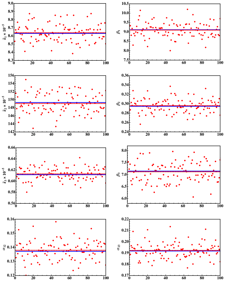
Figure 5: (color online) Results of sensitivity analysis for the effective parameters. The blue line, red line and red scattered points have the same meaning as in Fig. A1.

The resultant data of the sensitivity analysis are shown in Figs. A1-A2. The nature of the data shown in Figs. A1-A2 suggests that the parameter set obtained using the experimental switching values from Henke and Bassler (2004) is robust against small perturbations.

Glossary

Quorum sensing. Process leading to regulation of gene expression in response to cell density.

Autoinducers. Small signaling molecules produced by bacteria which bind to specific receptors and induce the quorum sensing response.

Kinase. Enzyme acting as phosphate donor.

Phosphatase. Enzyme acting as phosphate acceptor.

Bioluminescence. Production of light by living organism as a result of internal chemical reactions.

Vibrio harveyi. Gram-negative and bioluminescent marine bacterium.

References

References

- [1]
- [2] [] Appleby J L, Parkinson J S and Bourret R B 1996 Signal transduction via the multi-step phosphorelay: Not necessarily a road less traveled Cell 86 845
- [3]
- [4] [] Bassler B L and Losick R 2006 Bacterially speaking Cell 125 237
- [5]
- [6] [] Bjarnsholt T and Givskov M 2007 Quorum-sensing blockade as a strategy for enhancing host defences against bacterial pathogens Philos. Trans. R Soc. Lond. B 362 1213
- [7]
- [8] [] Freeman J A and Bassler B L 1999 A genetic analysis of the function of LuxO, a two-component response regulator involved in quorum sensing in Vibrio harveyi Mol. Microbiol. 31 665
- [9]
- [10] [] Freeman J A, Lilley B N and Bassler B L 2000 A genetic analysis of the functions of LuxN: a two-component hybrid sensor kinase that regulates quorum sensing in Vibrio harveyi Mol. Microbiol. 35 139
- [11]
- [12] [] Henke J M and Bassler B L 2004 Three parallel quorum-sensing systems regulate gene expression in Vibrio harveyi J. Bacteriol. 186 6902
- [13]
- [14] [] Hoch J A 2000 Two-component and phosphorelay signal transduction Curr. Opin. Microbiol. 3 165
- [15]
- [16] [] Laub M T and Goulian M 2007 Specificity in two-component signal transduction pathways Annu. Rev. Genet. 41 121
- [17]
- [18] [] Lenz D H, Mok K C, Lilley B N, Kulkarni R V, Wingreen N S and Bassler B L 2004 The small RNA chaperone Hfq and multiple small RNAs control quorum sensing in Vibrio harveyi and Vibrio cholerae Cell 118 69
- [19]
- [20] [] Levine E, Zhang Z, Kuhlman T and Hwa T 2007 Quantitative characteristics of gene regulation by small RNA PLoS Biol. 5 e229
- [21]
- [22] [] Levine E and Hwa T 2008 Small RNAs establish gene expression thresholds Curr. Opin. Microbiol. 11 574
- [23]
- [24] [] Mehta P, Goyal S and Wingreen N S 2008 A quantitative comparison of sRNA-based and protein-based gene regulation. Mol. Syst. Biol. 4 221
- [25]
- [26] [] Miller M B and Bassler B L 2001 Quorum sensing in bacteria Annu. Rev. Microbiol. 55 165
- [27]
- [28] [] Mitarai N, Andersson A M, Krishna S, Semsey S and Sneppen K 2007 Efficient degradation and expression prioritization with small RNAs Phys. Biol. 4 164
- [29]
- [30] [] Mok K C, Wingreen N S and Bassler B L 2003 Vibrio harveyi quorum sensing: a coincidence detector for two autoinducers controls gene expression EMBO J. 22 870
- [31]
- [32] [] Nealson K H, Platt T and Hastings J W 1970 Cellular control of the synthesis and activity of the bacterial luminescent system J. Bacteriol. 104 313
- [33]
- [34] [] Neiditch M B, Federle M J, Pompeani A J, Kelly R C, Swem D L, Jeffrey P D, Bassler B L and Hughson F M 2006 Ligand-induced asymmetry in histidine sensor kinase complex regulates quorum sensing Cell 126 1095
- [35]
- [36] [] Stock A M, Robinson V L and Goudreau P N 2000 Two-component signal transduction Annu. Rev. Biochem. 69 183
- [37]
- [38] [] Swem L R, Swem D L, Wingreen N S and Bassler B L 2008 Deducing receptor signaling parameters from in vivo analysis: LuxN/AI-1 quorum sensing in Vibrio harveyi Cell 134 461
- [39]
- [40] [] Timmen M, Bassler B L and Jung K 2006 AI-1 influences the kinase activity but not the phosphatase activity of LuxN of Vibrio harveyi J. Biol. Chem. 281 24398
- [41]
- [42] [] Tu K C and Bassler B L 2007 Multiple small RNAs act additively to integrate sensory information and control quorum sensing in Vibrio harveyi Genes. Dev. 21 221
- [43]
- [44] [] Waters C M and Bassler B L 2005 Quorum sensing: Cell-to-cell communication in bacteria Annu. Rev. Cell. Dev. Biol. 21 319
- [45]
- [46] [] Waters C M and Bassler B L 2006 The Vibrio harveyi quorum-sensing system uses shared regulatory components to discriminate between multiple autoinducers Genes. Dev. 20 2754
- [47]