How the Cosmological Constant Affects Gravastar Formation

Abstract

Here we generalized a previous model of gravastar consisted of an internal de Sitter spacetime, a dynamical infinitely thin shell with an equation of state, but now we consider an external de Sitter-Schwarzschild spacetime. We have shown explicitly that the final output can be a black hole, a ”bounded excursion” stable gravastar, a stable gravastar, or a de Sitter spacetime, depending on the total mass of the system, the cosmological constants, the equation of state of the thin shell and the initial position of the dynamical shell. We have found that the exterior cosmological constant imposes a limit to the gravastar formation, i.e., the exterior cosmological constant must be smaller than the interior cosmological constant. Besides, we have also shown that, in the particular case where the Schwarzschild mass vanishes, no stable gravastar can be formed, but we still have formation of black hole.

I Introduction

As alternatives to black holes, gravastars have received some attention recently grava1 grava2 , partially due to the tight connection between the cosmological constant and a currently accelerating universe DEs , although very strict observational constraints on the existence of such stars may exist BN07 .

The pioneer model of gravastar was proposed by Mazur and Mottola (MM) MM01 . After this work, Visser and Wiltshire (VW) VW04 pointed out that there are two different types of stable gravastars which are stable gravastars and ”bounded excursion” gravastars. The first one represents a stable structure already formed, while the second one is a system with a shell which oscillates around a equilibrium position which can loose energy and to stabilize at the end.

Recently we have done an extensive study on the problem of the stability of gravastars. The first model JCAP consisted of an internal de Sitter spacetime, a dynamical infinitely thin shell of stiff fluid, and an external Schwarzschild spacetime, as proposed by VW VW04 . We have shown explicitly that the final output can be a black hole, a ”bounded excursion” stable gravastar, a Minkowski, or a de Sitter spacetime, depending on the total mass $m$ of the system, the cosmological constant $\Lambda$, and the initial position $R_{0}$ of the dynamical shell. Therefore, we have shown, for the first time in the literature, that although it does exist a region of the space of the initial parameters where it is always formed stable gravastars, it still exists a large region of this space where we can find black hole formation. Then, we conclude that gravastar is not an alternative model to black hole as it was originally proposed by VW models VW04 .

In the second paper JCAP1 , we have generalized the previous work on the problem of stable gravastars considering an equation of state $p=(1-\gamma)\sigma$ for the shell, instead of only using a stiff fluid ($\gamma=0$). We have found that stable gravastars can be formed even for $\gamma\neq 0$, since $\gamma<1$, generalizing the gravastar models proposed until now. We also have confirmed the previous results, i.e., that both gravastars and black holes can be formed, depending on the initial parameters.

In the third work JCAP2 , we have generalized the former one considering now an interior constituted by an anisotropic dark energy fluid. We have again confirmed the previous results, i.e., that both gravastars and black holes can be formed, depending on the initial parameters. It is remarkable that for this case we have an interior fulfilled by a physical matter, instead of a de Sitter vacuum. Thus, it is similar to phantom energy star models.

Nowadays, several kinds of observational data indicate that our universe is in accelerated expansion. In Einstein’s general relativity, in order to have such an acceleration, one needs to introduce a component to the matter distribution of the universe with a large negative pressure. This component is usually referred as dark energy. Astronomical observations indicate that our universe is flat and currently consists of approximately $2/3$ dark energy and $1/3$ dark matter. The nature of dark energy as well as dark matter is unknown, and many radically different models have been proposed, such as, a tiny positive cosmological constant. Based on this fact, we would like to ask how the picture of the evolution of gravastar formation is influenced by an exterior spacetime with a positive cosmological constant.

Recently, Carter Carter studied spherically symmetric gravastar solutions which possess an (anti) de Sitter interior and a (anti) de Sitter-Schwarzschild or Reissner-Nordstrom exterior. He followed the same approach that Visser and Wiltshire took in their work VW04 assuming a potential $V(a)$ and then founding the equation of state of the shell. He found a wide range of parameters which allows stable gravastar solutions, and presented the different qualitative behaviors of the equation of state for these parameters.

Differently from Carter’s work Carter , we consider here another approach. We generalize our second work in gravastars JCAP1 , introducing an external de Sitter-Schwarzschild spacetime, to study how the cosmological constant affects the gravastar formation. We first assumed an equation of state, $p=(1-\gamma)\rho$, and, using Israel conditions, derived a potential depending on the parameters of the interior, the shell and the exterior of the gravastar’s prototype. We, then, studied the types of compact objects that can be generated according to this potential, to the parameters related to the cosmological constants and to the masses of our model. We found that both gravastars and black holes can be formed.

The paper is organized as follows: In Sec. II we present the metrics of the interior and exterior spacetimes, with theirs extrinsic curvatures, the equation of motion of the shell and the potential of the system. In Sec. III we discuss the particular cases where the Schwarzschild mass is null, and another where we have the same cosmological constant in the interior and the exterior of the thin shell, which is presented in section IV. In Sec. V we investigate the formation of gravastar from numerical analysis of the general potential. Finally, in Sec. VI we present our conclusions.

II Formation of Gravastars in a de Sitter-Schwarzschild spacetime

The interior spacetime is described by the de Sitter metric given by

$$ds^{2}_{i}=-f_{1}dt^{2}+f_{2}dr^{2}+r^{2}d\Omega^{2},$$ (1)

where $f_{1}=1-(r/L_{i})^{2}$, $f_{2}=\frac{1}{1-(ri/L_{i})^{2}}$, $L_{i}=\sqrt{3/\Lambda_{i}}$ and $d\Omega^{2}=d\theta^{2}+\sin^{2}(\theta)d\phi^{2}$.

The exterior spacetime is given by a de Sitter-Schwarzschild metric

$$ds^{2}_{e}=-fdv^{2}+f^{-1}d{\bf r}^{2}+{\bf r}^{2}d\Omega^{2},$$ (2)

where $f=1-\frac{2m}{\bf r}-({\bf r}/L_{e})^{2}$ and $L_{e}=\sqrt{3/\Lambda_{e}}$.

The metric of the hypersurface do the shell is given by

$$ds^{2}_{\Sigma}=-d\tau^{2}+R^{2}(\tau)d\Omega^{2}.$$ (3)

Since $ds^{2}_{i}=ds^{2}_{e}=ds^{2}_{\Sigma}$ then $r_{\Sigma}={\bf r}_{\Sigma}=R$, and besides

$$\dot{t}^{2} = \left[f_{1}-f_{2}\left(\frac{\dot{R}}{\dot{t}}\right)^{2}\right]^{-1}=$$ (4)

$$\left[1-\left(\frac{R}{L_{i}}\right)^{2}+\dot{R}^{2}\right]\left[1-\left(\frac{R}{L_{i}}\right)^{2}\right]^{-2},$$

and

$$\dot{v}^{2} = \left[f-f^{-1}\left(\frac{\dot{R}}{\dot{v}}\right)^{2}\right]^{-1}=$$ (5)

$$\left[1-\frac{2m}{R}-\left(\frac{R}{L_{e}}\right)^{2}+\dot{R}^{2}\right]\left[1-\frac{2m}{R}-\left(\frac{R}{L_{e}}\right)^{2}\right]^{-2},$$

where the dot represents the differentiation with respect to $\tau$.

Thus, the interior and exterior normal vector are given by

$$n^{i}_{\alpha}=(-\dot{R},\dot{t},0,0),$$ (6)

and

$$n^{e}_{\alpha}=(-\dot{R},\dot{v},0,0).$$ (7)

The interior and exterior extrinsic curvature are given by

$$K^{i}_{\tau\tau} = -[(3L_{i}^{4}\dot{R}^{2}-L_{i}^{4}\dot{t}^{2}+2L_{i}^{2}R^{2}\dot{t}^{2}-R^{4}\dot{t}^{2})R\dot{t}-(L_{i}+R)(L_{i}-R)(\dot{R}\ddot{t}-\ddot{R}\dot{t})L_{i}^{4}]\times$$ (8)

$$(L_{i}+R)^{-1}(L_{i}-R)^{-1}L_{i}^{-4}$$

$$K^{i}_{\theta\theta}=\dot{t}(L_{i}+R)(L_{i}-R)L_{i}^{-2}R$$ (9)

$$K^{i}_{\phi\phi}=K^{i}_{\theta\theta}\sin^{2}(\theta),$$ (10)

$$K^{e}_{\tau\tau} = \dot{v}[(2L_{e}^{2}m\dot{v}+L_{e}^{2}R\dot{R}-L_{e}^{2}R\dot{v}+R^{3}\dot{v})(2L_{e}^{2}m\dot{v}-L_{e}^{2}R\dot{R}-L_{e}^{2}R\dot{v}+R^{3}\dot{v})-$$ (11)

$$2L_{e}^{4}R^{2}\dot{R}^{2}]((2m-R)L_{e}^{2}+R^{3})^{-1}(L_{e}^{2}m-R^{3})L_{e}^{-4}R^{-3}+\dot{R}\ddot{v}-\ddot{R}\dot{v}$$

$$K^{e}_{\theta\theta}=-\dot{v}((2m-R)L_{e}^{2}+R^{3})L_{e}^{-2}$$ (12)

$$K^{e}_{\phi\phi}=K^{e}_{\theta\theta}\sin^{2}(\theta).$$ (13)

Since we have Lake

$$[K_{\theta\theta}]=K^{e}_{\theta\theta}-K^{i}_{\theta\theta}=-M,$$ (14)

where $M$ is the mass of the shell, thus

$$M=\dot{v}R\left[1-\frac{2m}{R}-\left(\frac{R}{L_{e}}\right)^{2}+\dot{R}^{2}\right]+\dot{t}R\left[1-\left(\frac{R}{L_{i}}\right)^{2}\right].$$ (15)

Then, substituting equations (4) and (5) into (15) we get

$$M+R\left[1-\frac{2m}{R}-\left(\frac{R}{L_{e}}\right)^{2}+\dot{R}^{2}\right]^{1/2}-R\left[1-\left(\frac{R}{L_{i}}\right)^{2}+\dot{R}^{2}\right]^{1/2}=0.$$ (16)

Solving the equation (16) for $\dot{R}^{2}/2$ we obtain the potential $V(R,m,L_{i},L_{e})$. In order to keep the ideas of our work JCAP1 as much as possible, we consider the thin shell as consisting of a fluid with a equation of state, $\sigma=(1-\gamma)\vartheta$, where $\sigma$ and $\vartheta$ denote, respectively, the surface energy density and pressure of the shell and $\gamma$ is a constant. The equation of motion of the shell is given by Lake

$$\dot{M}+8\pi R\dot{R}\vartheta=4\pi R^{2}[T_{\alpha\beta}u^{\alpha}n^{\beta}]=\pi R^{2}\left(T^{+}_{\alpha\beta}u_{+}^{\alpha}n_{+}^{\beta}-T^{-}_{\alpha\beta}u_{-}^{\alpha}n_{-}^{\beta}\right),$$ (17)

where $u^{\alpha}$ is the four-velocity. Since the interior and the exterior spacetimes correspond to vacuum solutions, we get

$$\dot{M}+8\pi R\dot{R}(1-\gamma)\sigma=0,$$ (18)

and since $\sigma=M/(4\pi R^{2})$ we can solve equation (18) giving

$$M=kR^{2(\gamma-1)},$$ (19)

where $k$ is an integration constant.

Substituting equation (19) into $V(R,m,L_{i},L_{e})$ we obtain

$$V(R,m,L_{i},L_{e},k,\gamma)=$$

$$-\frac{1}{8R^{2}L_{e}^{4}L_{i}^{4}k^{2}}\left[-4R^{2}L_{e}^{4}L_{i}^{4}k^{2}+4RmL_{e}^{4}L_{i}^{4}k^{2}+2R^{4}L_{i}^{4}k^{2}L_{e}^{2}+R^{(-4\gamma+12)}L_{e}^{4}\right.$$

$$\left.-4R^{(-4\gamma+9)}L_{e}^{4}L_{i}^{2}m-2R^{(-4\gamma+12)}L_{e}^{2}L_{i}^{2}+2R^{4}L_{e}^{4}L_{i}^{2}k^{2}+4R^{(-4\gamma+6)}L_{i}^{4}m^{2}L_{e}^{4}\right.$$

$$\left.+4R^{(-4\gamma+9)}L_{i}^{4}mL_{e}^{2}+R^{(-4\gamma+12)}L_{i}^{4}+R^{(4\gamma-4)}L_{i}^{4}k^{4}L_{e}^{4}\right].$$ (20)

Redefining the Schwarzschild mass $m$, the cosmological constants $L_{i}$ and $L_{e}$ and the radius $R$ as

$$m\equiv mk^{-\frac{1}{2\gamma-3}},$$ (21)

$$L_{i}\equiv L_{i}k^{\frac{2}{2\gamma-3}},$$ (22)

$$L_{e}\equiv L_{e}k^{\frac{2}{2\gamma-3}},$$ (23)

$$R\equiv Rk^{-\frac{1}{2\gamma-3}},$$ (24)

we get the potential

$$V(R,m,L_{i},L_{e},\gamma)=$$

$$-\frac{1}{2}\left[-1+\frac{m}{R}+\frac{R^{(4\gamma-6)}}{4}+m^{2}R^{(-4\gamma+4)}+\frac{R^{2}}{2L_{i}^{2}}-\frac{mR^{(-4\gamma+7)}}{L_{i}^{2}}+\frac{R^{(-4\gamma+10)}}{4L_{i}^{4}}-\right.$$

$$\left.-\frac{R^{(-4\gamma+10)}}{2L_{i}^{2}L_{e}^{2}}+\frac{R^{2}}{2L_{e}^{2}}+\frac{mR^{(-4\gamma+7)}}{L_{e}^{2}}+\frac{R^{(-4\gamma+10)}}{4L_{e}^{4}}\right].$$ (25)

Redefining $L_{e}=\alpha L_{i}$ we finally get

$$V(R,m,\alpha,L_{i},\gamma)=$$

$$-\frac{1}{2}\left[-1+\frac{m}{R}+\frac{R^{(4\gamma-6)}}{4}+m^{2}R^{(-4\gamma+4)}+\frac{R^{2}}{2L_{i}^{2}}-\frac{mR^{(-4\gamma+7)}}{L_{i}^{2}}+\frac{R^{(-4\gamma+10)}}{4L_{i}^{4}}-\right.$$

$$\left.-\frac{R^{(-4\gamma+10)}}{2\alpha^{2}L_{i}^{4}}+\frac{R^{2}}{2\alpha^{2}L_{i}^{2}}+\frac{mR^{(-4\gamma+7)}}{\alpha^{2}L_{i}^{2}}+\frac{R^{(-4\gamma+10)}}{4\alpha^{4}L_{i}^{4}}\right].$$ (26)

It is curious to note that this potential is independent of the sign of the parameter $\alpha$.

Therefore, for any given constants $m$, $\alpha$, $L_{i}$ and $\gamma$, equations (25) or (26) uniquely determines the collapse of the prototype gravastar. Depending on the initial value $R_{0}$, the collapse can form either a black hole, or gravastar, or a de Sitter spacetime. In the last case, the thin shell first collapses to a finite non-zero minimal radius and then expands to infinity. To guarantee that initially the spacetime does not have any kind of horizons, cosmological or event, we must restrict $R_{0}$ to the ranges simultaneously,

$$2m<R_{0}<L_{i},$$ (27)

$$2m<R_{0}<L_{e},$$ (28)

where $R_{0}$ is the initial collapse radius.

In order to fulfill the energy condition $\sigma+2p\geq 0$ of the shell and assuming that $p=(1-\gamma)\sigma$ we must have $\gamma\leq 1.5$. On the other hand, in order to satisfy the condition $\sigma+p\geq 0$, we get that $\gamma\leq 2$. The dominant energy condition is only satisfied for $0\leq\gamma\leq 2$. Although the phantom energy is usually considered as a kind of dark energy, in this paper we will use the expression dark energy for the case where the condition $\sigma+p\geq 0$ is satisfied and phantom energy otherwise. Hereinafter, we will use only some particular values of the parameter $\gamma$ which are analyzed in this work. See Table I.

Since the potential, equations (25) or (26), is very complex to manipulate analytically, we have analyzed several special cases.

Table 1: This table summarizes the matter classification based on the energy conditions of the shell, in terms of the parameter $\gamma$.

Matter	Condition 1	Condition 2	$\gamma$
Standard Energy	$\sigma+2p\geq 0$	$\sigma+p\geq 0$	$\gamma\leq 1.5$
Dark Energy	$\sigma+2p\leq 0$	$\sigma+p\geq 0$	$1.5\leq\gamma\leq 2$
Phantom Energy	$\sigma+2p\leq 0$	$\sigma+p\leq 0$	$\gamma\geq 2$

III Case $m=0$

This case represents a system where the Schwarzschild mass vanishes and the combination of both cosmological constant (interior and exterior) imposes a very special junction thin shell. Note that from equation (16), this configuration is possible only if $\alpha\neq 1$, otherwise if $\alpha=1$ then we have $M=0$, i.e., the thin shell vanishes.

From the equation (26) we get

$$\frac{1}{2}-\frac{R^{(4\gamma-6)}}{8}-\frac{R^{2}}{4L_{i}^{2}}-\frac{R^{(-4\gamma+10)}}{8L_{i}^{4}}+\frac{R^{(-4\gamma+10)}}{4\alpha^{2}L_{i}^{4}}-\frac{R^{2}}{4\alpha^{2}L_{i}^{2}}-\frac{R^{(-4\gamma+10)}}{8\alpha^{4}L_{i}^{4}}=0$$ (29)

and differentiating the potential $dV(R)/dR$, we get

$$-\frac{R^{(4\gamma-6)}(4\gamma-6)}{8R}-\frac{R}{2L_{i}^{2}}-\frac{R^{(-4\gamma+10)}(-4\gamma+10)}{8RL_{i}^{4}}+\frac{R^{(-4\gamma+10)}(-4\gamma+10)}{4R\alpha^{2}L_{i}^{4}}-$$

$$\frac{R}{2\alpha^{2}L_{i}^{2}}-\frac{R^{(-4\gamma+10)}(-4\gamma+10)}{8R\alpha^{4}L_{i}^{4}}=0.$$ (30)

From these two equations we can obtain the point where the potential has a minimum and equal to zero. Solving simultaneously the equations (29) and (30) we get

$$R_{c}=2^{-\frac{1}{2\gamma-3}}\left\{-\frac{2}{\alpha^{2}(-2+\gamma)}\left\{-2\alpha^{4}+\alpha^{4}\gamma-2\alpha^{2}\gamma+6\alpha^{2}+\gamma-2+\right.\right.$$

$$\left.\left.\left[(\alpha^{2}+1)^{2}(4\alpha^{4}+\alpha^{4}\gamma^{2}-4\alpha^{4}\gamma-7\alpha^{2}-2\alpha^{2}\gamma^{2}+8\alpha^{2}\gamma+4+\gamma^{2}-4\gamma)\right]^{\frac{1}{2}}\right\}\right\}^{\frac{1}{2(2\gamma-3)}},$$

$$L_{c}^{i}=-\frac{1}{(-4+R^{4\gamma-6})\alpha}\left\{-(-4+R^{4\gamma-6})\left[R^{2}\alpha^{2}+R^{2}+\left(R^{4}\alpha^{4}+2R^{4}\alpha^{2}+R^{4}+4R^{(-4\gamma+10)}-\right.\right.\right.$$

$$\left.\left.\left.8R^{(-4\gamma+10)}\alpha^{2}+4R^{(-4\gamma+10)}\alpha^{4}-R^{(4\gamma-6)}R^{(-4\gamma+10)}+2R^{(4\gamma-6)}R^{(4\gamma+10)}\alpha^{2}-R^{(4\gamma-6)}R^{(-4\gamma+10)}\alpha^{4}\right)^{\frac{1}{2}}\right]\right\}^{\frac{1}{2}}.$$

For $\alpha=\infty$ we get the same results of previous work JCAP1 , given by

$$R_{c}=\left|\frac{2(\gamma-2)}{2\gamma-5}\right|^{\frac{1}{3-2\gamma}},$$ (33)

and

$$L_{c}^{i}=\left|\frac{2\gamma-5}{2\gamma-3}\right|^{1/2}R_{c}^{2(2-\gamma)}.$$ (34)

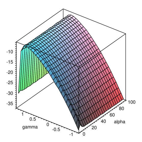
Figure 1: This plot shows, in terms of $\alpha$ and $\gamma$, the second derivative of the potential $V(R,m,\alpha,L_{i},\gamma)$ with respect to $R$, calculated at the values $R=R_{c}$ and $L_{i}=L_{c}^{i}$, in the intervals $-1.5<\gamma<1.5$ and $0<\alpha<100$, for $m=0$.

We can see from figure 1 that the quantity $V"(R)$, calculated at the values $R=R_{c}$ and $L_{i}=L_{c}^{i}$, is always negative, for a large range of values for $\alpha$ and $\gamma$ ($-1<\gamma<1.5$ and $0<\alpha<100$). This means that, if we impose $V(R)=V^{\prime}(R)=0$, we have always formation of black holes, instead of formation of stable gravastars.

In the next sections, we will analyze another interesting particular case, where $m\neq 0$ and $\alpha=1$.

IV Case $m\neq 0$ and $\alpha=1$

In this case we consider $L_{e}=L_{i}=L$ since $\alpha=1$.

From the equation (26) we get

$$-1+{\frac{m}{R}}+\frac{1}{4}\,{R}^{4\,y-6}+{m}^{2}{R}^{-4\,y+4}+{\frac{{R}^{2}}{{L}^{2}}}=0$$ (35)

and differentiating the potential $dV(R)/dR$, we get

$$-{\frac{m}{{R}^{2}}}+\frac{1}{4}\,{\frac{{R}^{4\,\gamma-6}\left(4\,\gamma-6\right)}{R}}+{\frac{{m}^{2}{R}^{-4\,\gamma+4}\left(-4\,\gamma+4\right)}{R}}+2\,{\frac{R}{{L}^{2}}}=0$$ (36)

From these two equations we can obtain the point where the potential has a minimum and equal to zero. Solving simultaneously the equations (35) and (36) we get

$$m_{c}={\frac{\left(-3+\sqrt{\left(25\,{R}^{4\,\gamma}+16\,{\gamma}^{2}{R}^{4\,\gamma}-40\,\gamma{R}^{4\,\gamma}+32\,{R}^{6}\gamma-16\,{R}^{6}\right){R}^{-4\,\gamma}}\right){4R}^{4\,\gamma}}{{R}^{5}\left(2\,\gamma-1\right)}},$$ (37)

$$L_{c}^{2}=$$

$${\frac{-8{R}^{13-8\,\gamma}\left(2\,\gamma-1\right)^{2}}{16\,{R}^{11-8\,\gamma}(3\gamma-2\gamma^{2}-1)+(4\gamma-5){R}^{-4\,\gamma+5}[4\gamma-5+\sqrt{(4\gamma-5)^{2}+16\,{R}^{-4\,\gamma+6}(2\gamma-1)}]}}.$$

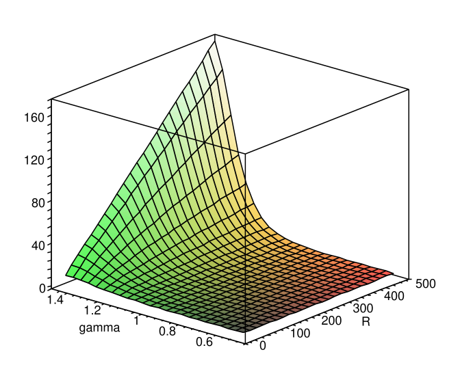
Figure 2: This plot shows that, in terms of $R$ and $\gamma$ and for $L_{e}=L_{i}$, the critical mass $m_{c}$ is always negative, when $V(R)=0$ and $V^{\prime}(R)=0$, for the interval $0.5<\gamma<1.5$, since the critical mass is not defined for $\gamma<0.5$.

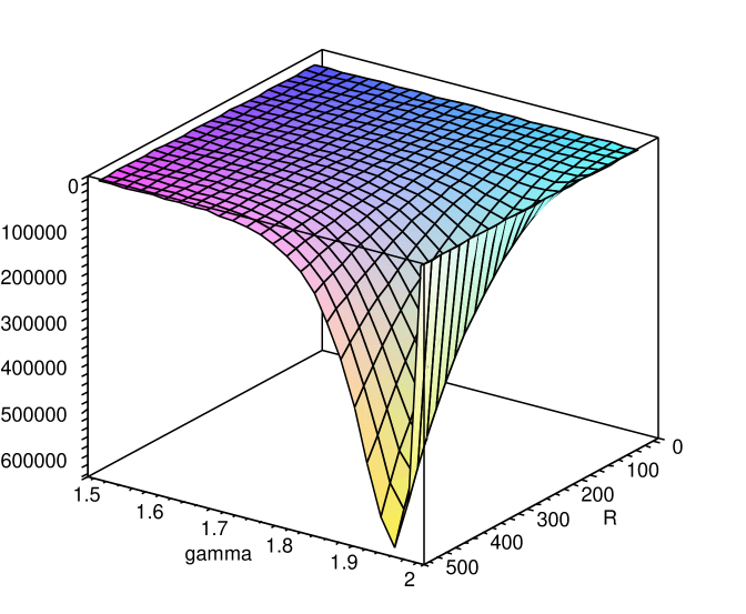
Figure 3: This plot shows that, in terms of $R$ and $\gamma$ and for $L_{e}=L_{i}$, the critical mass $m_{c}$ is always negative, when $V(R)=0$ and $V^{\prime}(R)=0$, for the interval $1.5<\gamma<2$.

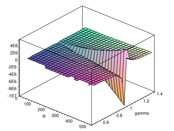
Figure 4: This plot shows, in terms of $R$ and $\gamma$, the cosmological constants $L_{e}=L_{i}$ when $V(R)=0$ and $V^{\prime}(R)=0$, for the interval $0.5<\gamma<1.5$, since the cosmological constant is not defined for $\gamma<0.5$. The critical mass $m_{c}$ is always negative for $1.5<\gamma<2.0$.

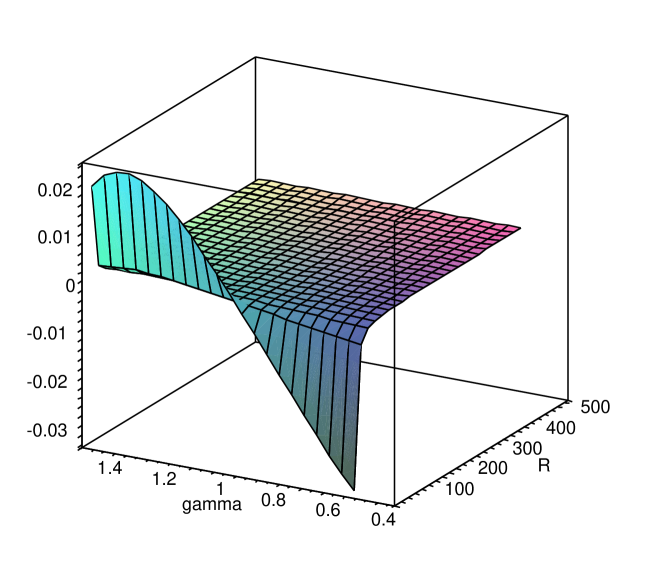
Figure 5: This plot shows, in terms of $\alpha$ and $\gamma$, the second derivative of the potential $V(R,m,\alpha=1,L_{i},\gamma)$ with respect to $R$, calculated at the values $R=R_{c}$ and $L_{i}=L_{c}^{i}$, for the interval $0.4<\gamma<1.5$, since the derivative is not defined for $\gamma<0.5$.

From the figures 2 and 3 we can see that the critical mass $m_{c}$ is positive only in the range $0.5\leq\gamma\leq 1.5$. Besides, from the figure 4 we can note that there is not any real value for the critical cosmological constant $L_{c}$ in the interval $\gamma\leq 1$. As a consequence of these results, the second derivative of the potential $V"(R)$, shown in the figure 5, is negative for $\gamma<1$ and positive for $1<\gamma\leq 1.5$. For $\gamma=1$ we have $V"(R)=0$ implying that we have an inflection point in the potential.

Combining all these facts, we conclude that for $L_{e}=L_{i}$ we obtain the following:

1. For $\gamma>1.5$, which corresponds to a dark energy shell, none structure is formed.

2. For $0.5\leq\gamma\leq 1.5$, which corresponds to a standard fluid shell, it can collapse to a black hole ($0.5\leq\gamma<1$), or it does not collapse, reaching an equilibrium stage, forming a stable gravastar ($1<\gamma\leq 1.5$).

3. For $\gamma=1$ none gravastar is formed.

Then, for $\alpha=1$, we have shown that no stable gravastar can exist, for $\gamma\leq 0.5$.

V General Case

The expressions for the potentials in the present case makes difficult a complete analytic analysis, so we shall study it numerically. Our main strategy is to start with the values of $m_{c}$ obtained for the case studied in our previous work JCAP1 , where $m\neq 0$ and $L_{i}\neq\infty$, and then gradually turn on $L_{e}$. The potential $V(R,m_{c},L_{i},L_{e},\gamma)$ is plotted as a function of $R$, by finely tuning $L_{e}$ until a stable gravastar or a ”bounded excursion” gravastar is found. We also made another approach, solving the system of equations $V(R,m_{c},L_{i},L_{e},\gamma)=0$ and $V^{\prime}(R,m_{c},L_{i},L_{e},\gamma)=0$ for $R$ and $L_{e}$ and fixing the parameters $m_{c}$, $L_{i}$ and $\gamma$ in order to compare the results we obtained for $L_{e}$. It was seen that there is a range of $L_{e}$ in which ”bounded excursion” stable gravastars are found, i.e., $L_{e}^{min}<L_{e}<L_{e}^{max}$. For $L_{e}\geq L_{e}^{max}$ we have found only stable gravastars.

We must call attention to the fact that, hereinafter, we will not consider the physical situation where there is dispersion of the star. If the initial radius of the collapse is greater enough, the star will first contract to its minimal radius and then expand to infinity, whereby a de Sitter spacetime is finally formed.

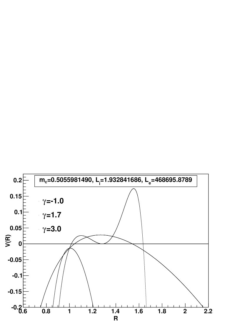
Figure 11: The potential $V(R)$ for $\gamma=-1$, $m_{c}=0.5055981490$, $L_{i}=1.932841686$ and $L_{e}^{max}=468695.8789$. (the curve that has a minimum). The others two curves top-down use the values $\gamma=1.7$ and $\gamma=3$, respectively. Cases B and D

Figures 6-11 show the behavior of the potential as a function of $R$ for the case where $\gamma=-1$. This case was not studied on our previous work JCAP1 where there was no cosmological constant external to the thin shell. So, we used the analytic expression (2.23) from our previous work JCAP1 to calculate $m_{c}$. This situation is analogous to our present work if we use the potential with $L_{i}=L_{e}=\infty$. The potential is shown in figure 6 where $m_{c}\approx 0.5055981490$ and $R_{c}\approx 1.023836256$. For $m>m_{c}$ the potential $V(R)$ is strictly negative and the collapse always forms black holes. For $m=m_{c}$, there are two different possibilities, depending on the choice of the initial radius $R_{0}$. In particular, if the star begins to collapse with $R_{0}>R_{c}$, the collapse will asymptotically approach the minimal radius $R_{c}$. Once it collapses to this point, the shell will stop collapsing and remains there for ever. However, in this case this point is unstable and any small perturbations will lead the star either to expand for ever and leave behind a flat spacetime, or to collapse until $R=0$, whereby a Schwarzschild black hole is finally formed. On the other hand, if the star begins to collapse with $2m_{c}<R_{0}<R_{c}$, the star will collapse until a black hole is formed. For $m<m_{c}$, the potential $V(R)$ have a positive maximum, and the equation $V(R,m<m_{c})=0$ has two positive roots $R_{1,2}$ with $R_{2}>R_{1}>0$. There are two possibilities here, depending on the choice of the initial radius $R_{0}$. If $R_{0}>R_{2}$, the star will first collapse to its minimal radius $R=R_{2}$ and the expand to infinity, whereby a Minkowski spacetime is finally formed. If $2m_{c}<R_{0}<R_{1}$, the star will collapse continously until R=0, and a black hole will be finally formed. As we always have $V^{\prime\prime}<0$, it means that no stable stars exist in this case.

For the case of the figure 6, i.e, $m=0.5055981490$, $L_{i}=L_{e}=\infty$ and $\gamma=-1$, we have analyzed the behavior of the potential for the parameter $\gamma=0.7,1.7,3$ and we have found that we get only dispersion of the shell.

The figures 7 and 8 show the case where $L_{e}=\infty$, but $L_{i}\neq\infty$. Variations of $m$ fixing the parameter $L_{i}$ and variations of $L_{i}$ fixing the parameter $m$ reveal that both stable gravastars and ”bounded excursion” stable gravastars can be formed, but not excluding the existence of black holes.

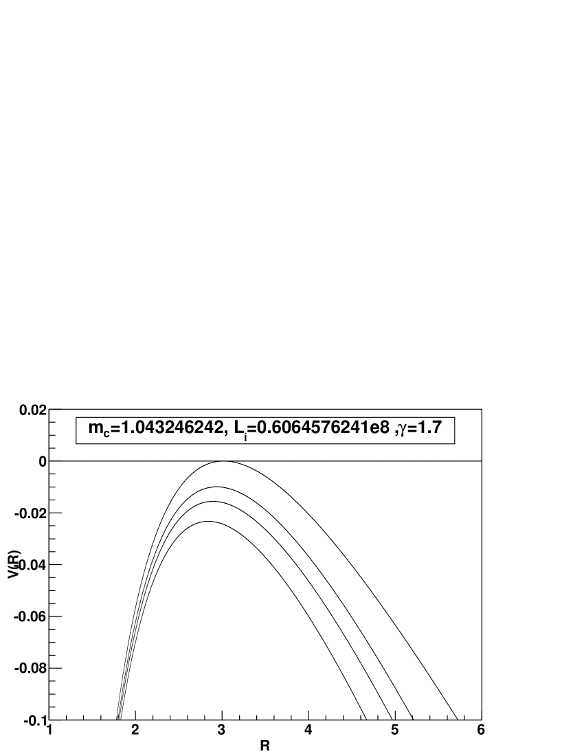
Figure 15: The potential $V(R)$ for $\gamma=1.7$, $L_{i}=0.6064576241\times 10^{8}$ and $m_{c}=1.043246242$ (the first curve top-down). The others curves represent $m>m_{c}$. The potential is insensible for variations of $L_{e}$. These curves generalize the results presented in the figure 20 from JCAP1 . Case C

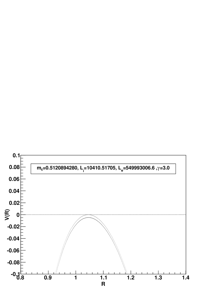
Figure 16: The potential $V(R)$ for $\gamma=3$, $L_{e}=549993006.6$, $L_{i}=10410.51705$ and $m_{c}=0.5120894280$ (the first curve top-down). The second curve represent $m>m_{c}$. Case D

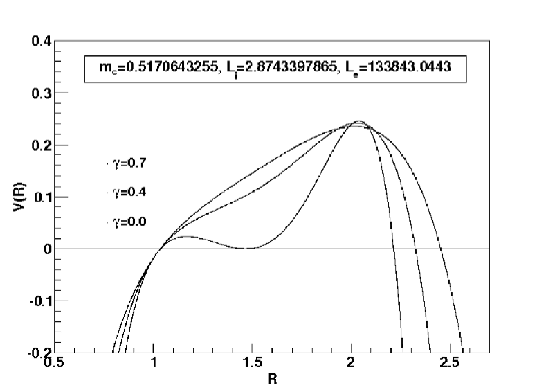
Figure 17: The potential $V(R)$ for $\gamma=0.7$, $L_{e}=133843.0443$, $L_{i}=2.8743397865$ and $m_{c}=0.5170643255$ (the first curve top-down). The second curve top-down is calculated using $\gamma=0.4$. The third curve top-down is obtained assuming $\gamma=0$. Case B

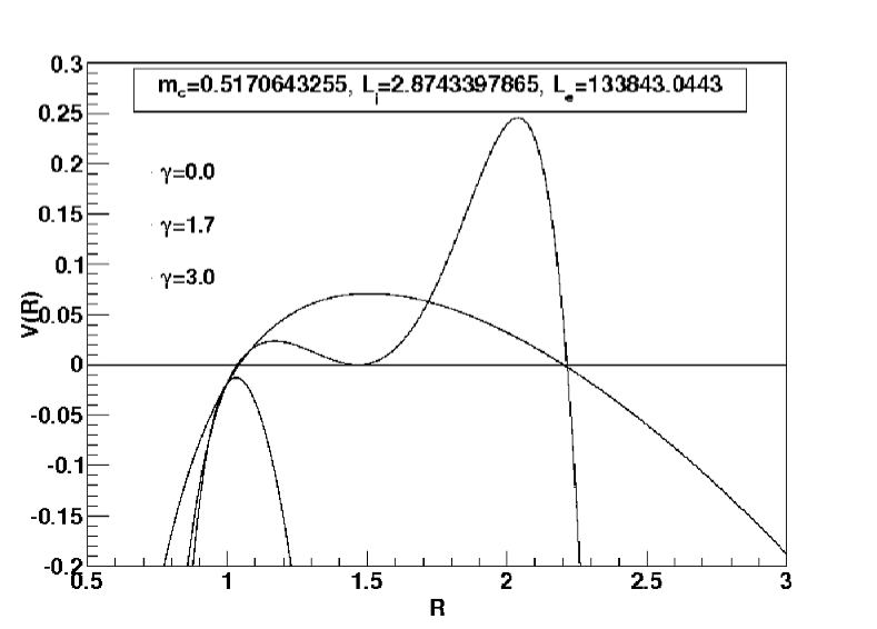
Figure 18: The potential $V(R)$ for $\gamma=0$, $L_{e}=133843.0443$, $L_{i}=2.8743397865$ and $m_{c}=0.5170643255$ (the first curve top-down). The second curve top-down is calculated using $\gamma=1.7$. The third curve top-down is obtained assuming $\gamma=3$. Case D

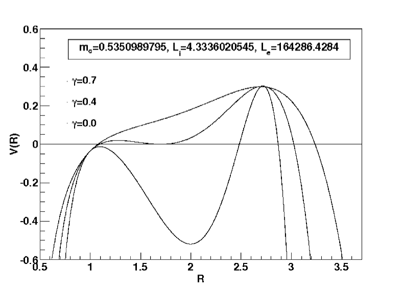
Figure 19: The potential $V(R)$ for $\gamma=0.7$, $L_{e}=164286.4284$, $L_{i}=4.3336020545$ and $m_{c}=0.5350989795$ (the first curve top-down). The second curve top-down is calculated using $\gamma=0.4$. The third curve top-down is obtained assuming $\gamma=0$. Case B

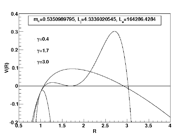
Figure 20: The potential $V(R)$ for $\gamma=0.4$, $L_{e}=164286.4284$, $L_{i}=4.3336020545$ and $m_{c}=0.5350989795$ (the first curve top-down). The second curve top-down is calculated using $\gamma=1.7$. The third curve top-down is obtained assuming $\gamma=3$. Case D

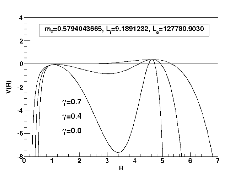
Figure 21: The potential $V(R)$ for $\gamma=0.7$, $L_{e}=127780.9030$, $L_{i}=9.1891232$ and $m_{c}=0.5794043665$ (the first curve top-down). The second curve top-down is calculated using $\gamma=0.4$. The third curve top-down is obtained assuming $\gamma=0$. Case B

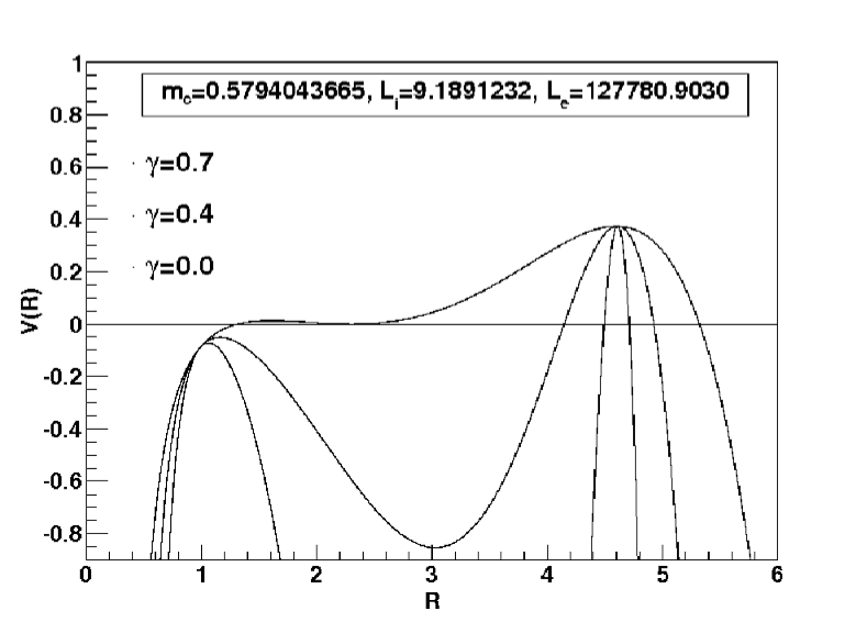
Figure 22: The potential $V(R)$ for $\gamma=0.7$, $L_{e}=127780.9030$, $L_{i}=9.1891232$ and $m_{c}=0.5794043665$ (the first curve top-down). The second curve top-down is calculated using $\gamma=0.4$. The third curve top-down is obtained assuming $\gamma=0$. Case B

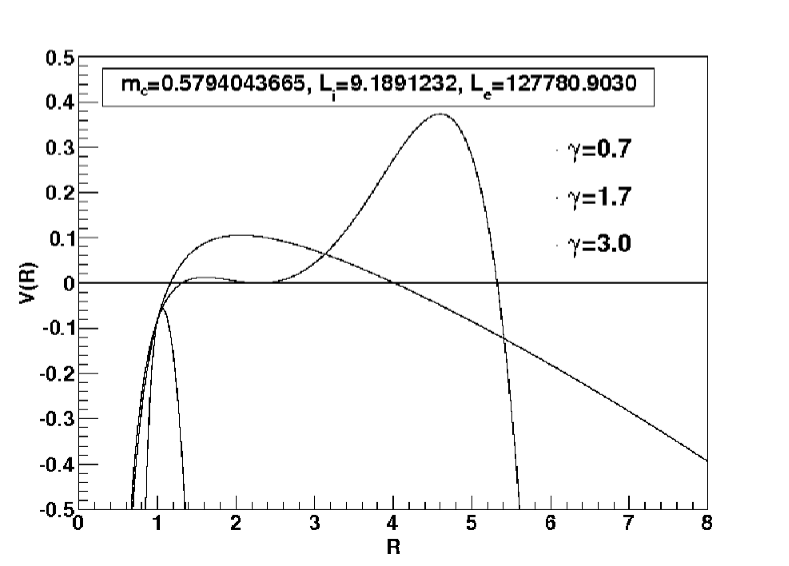
Figure 23: The potential $V(R)$ for $\gamma=0.7$, $L_{e}=127780.9030$, $L_{i}=9.1891232$ and $m_{c}=0.5794043665$ (the first curve top-down). The second curve top-down is calculated using $\gamma=1.7$. The third curve top-down is obtained assuming $\gamma=3$. Case D

For the general case, where both $L_{i}$ and $L_{e}$ are not infinity, it is shown the potential $V(R)$ as a function of $R$ for some specific values of $\gamma$, which are $\gamma=-1$, $\gamma=0$, $\gamma=0.4$ and $\gamma=0.7$ representing standard energy, $\gamma=1.7$ representing dark energy and $\gamma=3$ for phantom energy. Note that $\gamma=-1$ and $\gamma=3$ violate the dominant energy condition. Note also that in the Carter’s work Carter , the dominant energy condition is considered to restrict acceptable solutions. In our case this corresponds to the cases $\gamma=0$, 0.4, 0.7 and $\gamma=1.7$. We found that the shell must have standard energy (figures 9, 12, 13 and 14) in order to have both stable gravastars or ”bounded excursion” stable gravastars (the later existing whenever $L_{e}^{min}<L_{e}<L_{e}^{max}$ as explained in the text), but never excluding the existence of black holes or the formation of a de Sitter space depending on the choice of initial radius $R_{0}$ (It is important to verify the restriction on the values $R_{0}$ can assume, obeying both $2m<R_{0}<L_{i}$ and $2m<R_{0}<L_{e}$.). For dark energy shells and for phantom energy shells there are not formation of gravastars (figures 15 and 16). Variations of $\gamma$ in the potentials studied also show that when the region of $\gamma$ represents dark or phantom energy, there are only possibilities of formation of black holes or de Sitter spacetime (figures 11, 18, 20 and 23). When the shell is made of standard energy we can have gravastars or black holes (figures 10, 17, 19, 21 and 22). Thus, we only find gravastars for standard energy shells, satisfying or not the dominant energy conditions.

Table 2: This table summarizes all possible kind of energy of the interior fluid and of the shell. M, S, dS and dSS denote Minkowski, Schwarzschild, de Sitter and de Sitter-Schwarzschild spacetimes, respectively.

Case	Interior	Shell Energy	Exterior	Figures	Conditions	Structures
A	M	Standard	S	6	$m>m_{c}$	Black Hole
B	dS	Standard	S	7	$m=m_{c}$, $m=0.51$	Gravastar
				7	$m=0.53$	Black Hole
				8	$L_{i}=L_{c}$, $L_{i}=1.4$	Gravastar
				8	$L_{i}=1.0$	Black Hole
			dSS	9, 12, 13, 14	${L_{e}}^{mim}<L_{e}<{L_{e}}^{max}$	Gravastar
				9, 12, 13, 14	$L_{e}\leq{L_{e}}^{min}$	Black Hole
				10, 11	$\gamma=-1$	Gravastar
				17	$\gamma=0.0$	Gravastar
				19, 21	$\gamma=0.4$	Gravastar
				19, 21	$\gamma=0.0$	Black Hole
				22	$\gamma=0.7$	Gravastar
				22	$\gamma=0.0,0.4$	Black Hole
C	dS	Dark	dSS	15	$m>m_{c}$	Black Hole
D	dS	Phantom	dSS	11, 18, 20, 23	$\gamma=3$	Black Hole
				16	$m>m_{c}$	Black Hole

VI Conclusions

In this paper, we have generalized the problem of the stability of gravastars studied recently by us JCAP1 , introducing a positive cosmological constant in the exterior spacetime. Thus, the model consists of a de Sitter interior spacetime, a dynamical infinitely thin shell of fluid with an equation of state $p=(1-\gamma)\sigma$, and an external de Sitter-Schwarzschild spacetime. We have shown explicitly that the final output can be a black hole, a ”bounded excursion” stable gravastar, a stable gravastar, or a de Sitter spacetime, depending on the total mass $m$ of the system, the parameter $\alpha$, the constant $L_{i}$, the parameter of the shell $\gamma$ and the initial position $R_{0}$ of the dynamical shell. All these possibilities have non-zero measurements in the parameter space of $m$, $L_{i}$, $\alpha$, $\gamma$ and $R_{0}$, for both gravastar and black hole.

For $m=0$, the analysis of the potential has shown that, if we impose $V(R)=V^{\prime}(R)=0$, we have always formation of black holes, instead of formation of stable gravastars. Comparing the results from JCAP1 ($L_{e}=\infty$) with this work, we have confirmed that, in a more general way, there is no formation of gravastar even with the introduction of a $L_{e}\neq\infty$.

On the other hand, for $m\neq 0$, if $L_{i}=L_{e}$ ($\alpha=1$) we have formation of black hole or stable gravastar. These gravastars are only possible for $1<\gamma\leq 1.5$, satisfying all the dominant energy conditions. It is interesting to remark that this case can not be compared to other one already studied by us JCAP1 , except for $L_{i}=L_{e}=\infty$, which was shown in the figures 6 and 7, in that paper, and in the figure 6 of this work. While we have gravastars there for $\gamma<1$, here the gravastar formation is limited to $1<\gamma\leq 1.5$, showing that these intervals are complementary to each other, except for $\gamma=1$.

In the general case, i.e., $m\neq 0$, $L_{i}\neq L_{e}$, it was seen that there is a range of $L_{e}$ in which ”bounded excursion” stable gravastars are found, i.e., $L_{e}^{min}<L_{e}<L_{e}^{max}$. (Reminding that the curve for $L_{e}=\infty$ is very close to the curve for $L_{e}=L_{e}^{max}$.) Stable gravastars were found for $L_{e}\geq L_{e}^{max}$. Besides, this interval depends on the values of $L_{i}$ and $\gamma$. Let us now compare figures 12 and 13 , presented here, with figures 8 and 10, from JCAP1 , respectively. We can state that, from figures 8 and 10 JCAP1 , the bigger is $L_{i}$ (for $L_{e}=\infty$) the bigger is the tendency to the collapse of the shell, forming a ”bounded excursion” gravastar or a black hole. Moreover, from figures 9, 12, 13 and 14 of this paper, for a given $L_{i}$, the formation of gravastars depends on the value of $L_{e}$ ($L_{e}>{L_{e}}^{min}$, with ${L_{e}}^{min}\geq L_{i}$) in a such way that, instead of what occurs for $L_{i}$, the smaller is $L_{e}$ the bigger is the tendency to the collapse. These conclusions are in agreement to the gravastar requirement proposed by Horvat & Ilijic grava1 . The reason is that the dark energy density inside the gravastar have to be greater than the surround spacetime, i.e., $L_{i}<L_{e}$. All these results can be summarized in Table II.

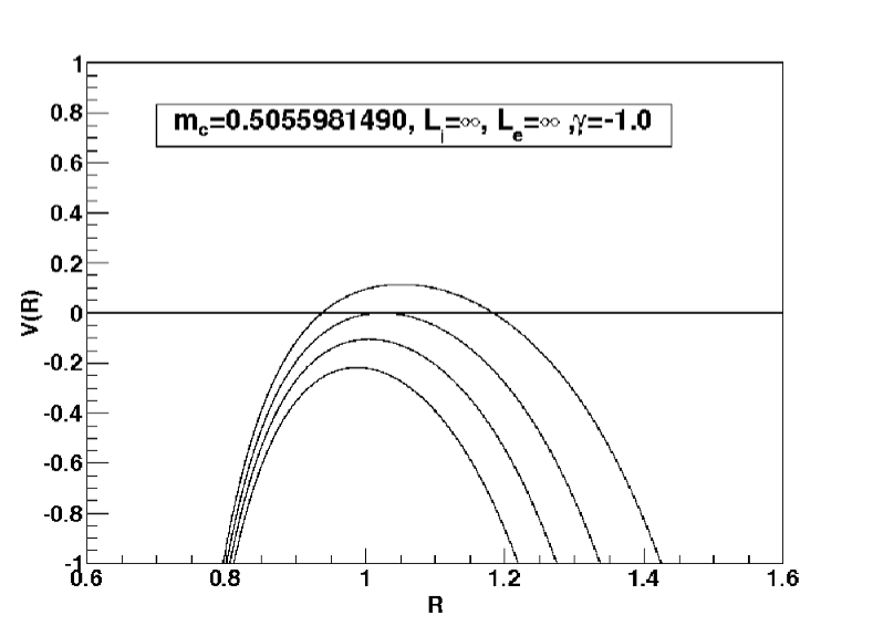
Figure 6: The potential $V(R)$ for $\gamma=-1$, $m_{c}=0.5055981490$, $L_{e}=\infty$, and $L_{i}=\infty$ (the second curve top-down). The others curves represent values for $m<m_{c}$ (first curve top-down) and $m>mc$ (the third and fourth curve top-down). Case A

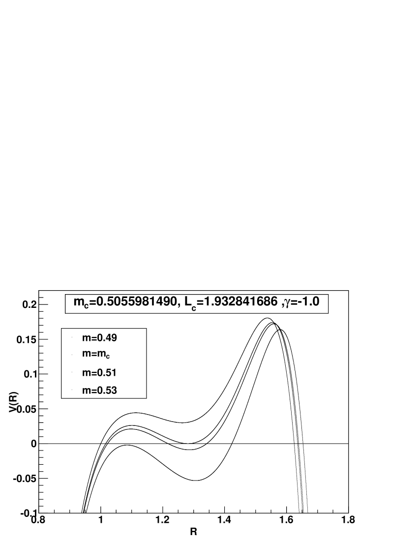
Figure 7: The potential $V(R)$ for $\gamma=-1$, $m_{c}=0.5055981490$, $L_{i}=L_{c}=1.932841686$ and $L_{e}=\infty$ (second curve top-down). The first curve top-down assumes $m=0.49$. The third and fourth curves top-down assume $m=0.51$ and $m=0.53$, respectively. Case B

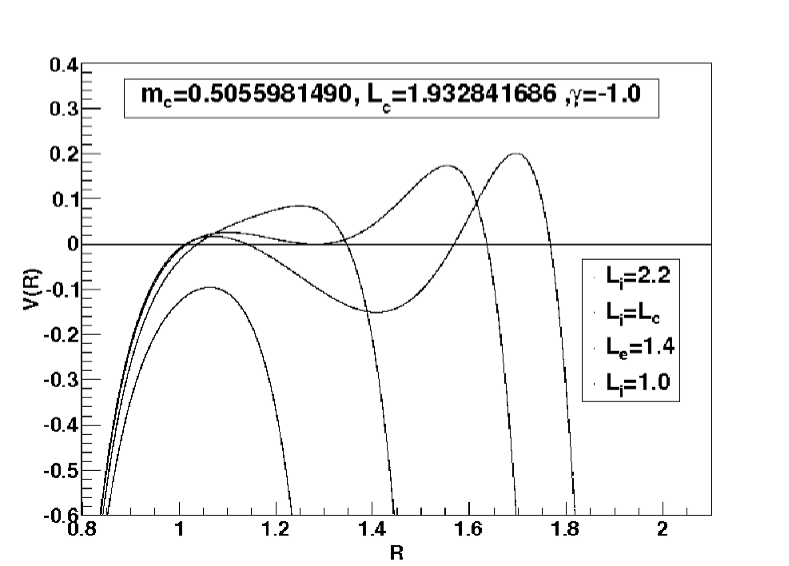
Figure 8: The potential $V(R)$ for $\gamma=-1$, $m_{c}=0.5055981490$, $L_{i}=1.932841686$ and $L_{e}=\infty$ (the second curve top-down). The first curve assumes $L_{i}=1.4$. The third and fourth curves top-down assume $L_{i}=2.2$ and $L_{i}=1.0$, respectively. Case B

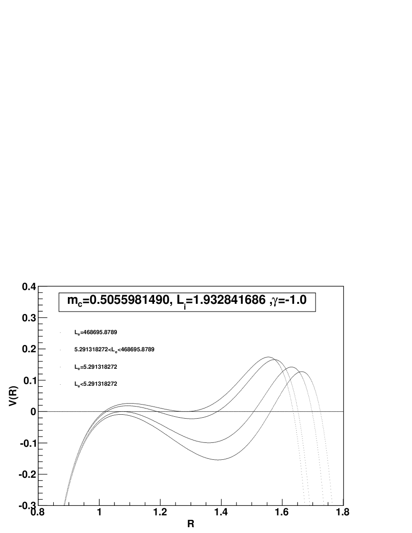
Figure 9: The potential $V(R)$ for $\gamma=-1$, $m_{c}=0.5055981490$, $L_{i}=1.932841686$ and $L_{e}=L_{e}^{max}=468695.8789$ (the first curve top-down). The second curve top-down is calculated using $5.291318272<L_{e}<468695.8789$. The third curve top-down is obtained assuming $L_{e}=5.291318272$. The fourth curve top-down assumes $L_{e}<5.291318272$. The curve for $L_{e}=\infty$ is very close to the curve for $L_{e}=L_{e}^{max}$. Case B

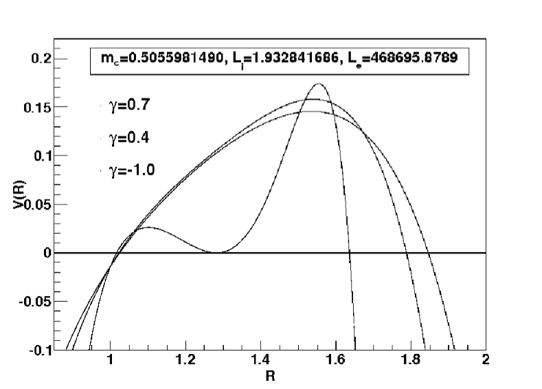
Figure 10: The potential $V(R)$ for $\gamma=-1$, $m_{c}=0.5055981490$, $L_{i}=1.932841686$ and $L_{e}=L_{e}^{max}=468695.8789$ (the curve that has a minimum). The others two curves top-down use the values $\gamma=0.7$ and $\gamma=0.4$, respectively. Case B

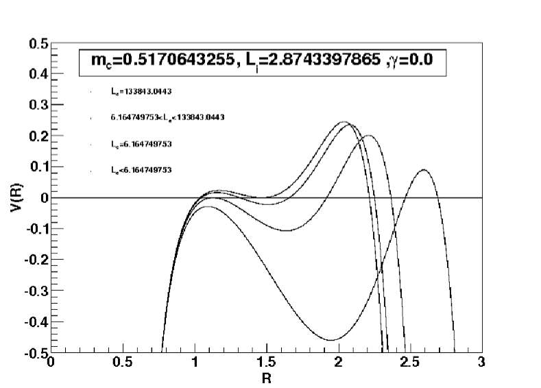
Figure 12: The potential $V(R)$ for $\gamma=0$, $L_{e}=133843.0443$, $L_{i}=2.8743397865$ and $m_{c}=0.5170643255$ (the first curve top-down). The second curve top-down is calculated using $6.16479753<L_{e}<133843.0443$. The third curve top-down is obtained assuming $L_{e}=6.16479753$. The fourth curve top-down assumes $L_{e}<6.164749753$. The curve for $L_{e}=\infty$ is very close to the curve for $L_{e}=L_{e}^{max}$. These curves generalize the results presented in the figure 8 from JCAP1 . Case B

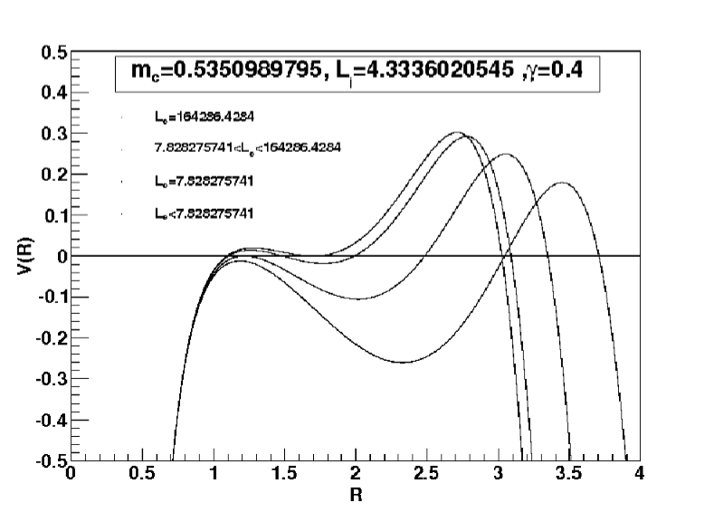
Figure 13: The potential $V(R)$ for $\gamma=0.4$, $L_{e}=164286.4284$, $L_{i}=4.3336020545$ and $m_{c}=0.5350989795$ (the first curve top-down). The second curve top-down is calculated using $7.828275741<L_{e}<164286.4284$. The third curve top-down is obtained assuming $L_{e}=7.828275741$. The fourth curve top-down assumes $L_{e}<7.828275741$. The curve for $L_{e}=\infty$ is very close to the curve for $L_{e}=L_{e}^{max}$. These curves generalize the results presented in the figure 10 from JCAP1 . Case B

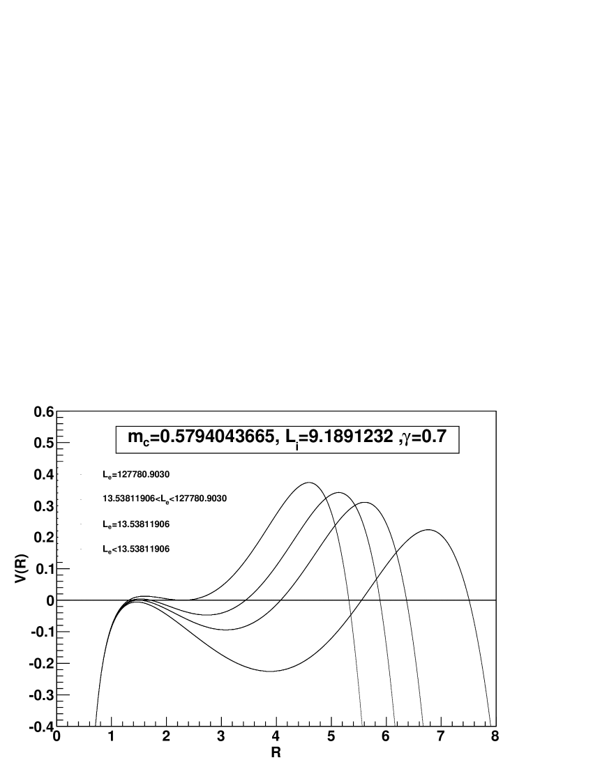
Figure 14: The potential $V(R)$ for $\gamma=0.7$, $L_{e}=127780.9030$, $L_{i}=9.1891232$ and $m_{c}=0.5794043665$ (the first curve top-down). The second curve top-down is calculated using $13.53811906<L_{e}<127780.9030$. The third curve top-down is obtained assuming $L_{e}=13.53811906$. The fourth curve top-down assumes $L_{e}<13.53811906$. The curve for $L_{e}=\infty$ is very close to the curve for $L_{e}=L_{e}^{max}$. These curves generalize the results presented in the figure 12 from JCAP1 . Case B

References

(1) D. Horvat and S. Ilijic, arXiv:0707.1636.
(2) P. Marecki, arXiv:gr-qc/0612178;
F.S.N. Lobo, Phys. Rev. D75, 024023 (2007); arXiv:gr-qc/0612030;
Class. Quantum Grav. 23, 1525 (2006);
F.S.N. Lobo, Aaron V. B. Arellano, ibid., 24, 1069 (2007);
T. Faber, arXiv:gr-qc/0607029;
C. Cattoen, arXiv:gr-qc/0606011;
O.B. Zaslavskii, Phys. Lett. B634, 111 (2006);
C. Cattoen, T. Faber, and M. Visser, Class. Quantum Grav. 22, 4189 (2005).
(3) E.J. Copeland, M. Sami and S. Tsujikawa, Int. J. Mod. Phys. D15, 1753 (2006);
T. Padmanabhan, arXiv:07052533.
(4) A.E. Broderick and R. Narayan, Class. Quantum Grav. 24, 659 (2007)
[arXiv:gr-qc/0701154].
(5) P.O. Mazur and E. Mottola, ”Gravitational Condensate Stars: An Alternative to
Black Holes,” arXiv:gr-qc/0109035; Proc. Nat. Acad. Sci. 101, 9545
(2004) [arXiv:gr-qc/0407075].
(6) M. Visser and D.L. Wiltshire, Class. Quantum Grav. 21, 1135 (2004)[arXiv:gr-qc/0310107].
(7) P. Rocha, A.Y. Miguelote, R. Chan, M.F.A. da Silva, N.O. Santos,, and A. Wang,
J. Cosmol. Astropart. Phys. 6, 25 (2008) [arXiv:gr-qc/08034200].
(8) P. Rocha, R. Chan, M.F.A. da Silva and A. Wang,
J. Cosmol. Astropart. Phys. 11, 10 (2008) [arXiv:gr-qc/08094879].
(9) R. Chan, M.F.A. da Silva, P. Rocha and A. Wang,
J. Cosmol. Astropart. Phys. 3, 10 (2009) [arXiv:gr-qc/08124924].