Higher coordination with less control – A result of information maximization in the sensorimotor loop

Abstract

This work presents a novel learning method in the context of embodied artificial intelligence and self-organization, which has as few assumptions and restrictions as possible about the world and the underlying model. The learning rule is derived from the principle of maximizing the predictive information in the sensorimotor loop. It is evaluated on robot chains of varying length with individually controlled, non-communicating segments. The comparison of the results shows that maximizing the predictive information per wheel leads to a higher coordinated behavior of the physically connected robots compared to a maximization per robot. Another focus of this paper is the analysis of the effect of the robot chain length on the overall behavior of the robots. It will be shown that longer chains with less capable controllers outperform those of shorter length and more complex controllers. The reason is found and discussed in the information-geometric interpretation of the learning process.

Keywords: Predictive Information, Embodied Artificial Intelligence, Sensorimotor Loop, Self-Organized Learning, Information Theory

1 Introduction

An ongoing research topic is to understand the learning and adaptation processes of cognitive systems. This paper will not define what a cognitive system is. Instead, the term cognitive system is used as an abstract concept just as in (Brooks, 1991). Generally speaking, in this context, cognition is understood as a process that transforms sensory data into motor commands using some form of internal (non-symbolic) representation (Förster, 1993). Hence, cognition is a process which lives in the sensorimotor loop (Cliff, 1990), or, otherwise stated, to understand adaptation and learning it is essential to take the body and environment into account (Pfeifer  Bongard, 2006). In order to investigate learning and adaptation, this work follows the approach of embodied artificial intelligence, first described by Brooks (1986) and later refined by Pfeifer  Bongard (2006), in which complete robotic systems of lower complexity are built and understood before the complexity is then gradually increased.

In the field of embodied artificial intelligence, learning and adaptation rules are very often specific in either their possible applications or applicable models (with few exceptions, such as (Pasemann ., 2004)). Examples are the ISO/ICO learning (Porr, 2003) which is limited to a single neuron network, and the Homeostatic learning rule by Di Paolo (2000), which operates on a fully connected recurrent neural network, but requires a trigger mechanism. We are interested in a first principle learning rule, i.e. a learning rule which is independent of the model structure and requires as few assumptions as possible about the morphology and environment. This sounds like a contradiction to the statement of the first paragraph (the sensorimotor loop is essential to understand cognition), and therefore, needs to be elaborated. We are looking at a very basic level of unsupervised and self-organized learning, i.e. before any task-dependent learning occurs. The question is, how can a system, with no knowledge of itself or the world, learn enough to perform coordinated interactions within the environment? An analogy is an infant who performs what is known as motor- or body babbling in order to learn how to produce facial expressions (Meltzoff  Moore, 1997). Clark (1996) describes it more generally, and states that there is evidence by Thelen  Smith (1996), that infants learn about the world through actions (and that the acquired knowledge is also action-specific). It is this form of learning that we are interested in.

We can now reformulate and specify the question above as the question of how a system may interactively gain maximal information about itself and the world. This is related to other self-motivated learning approaches. An example, and probably the first implementation is (Schmidhuber, 1990), in which, additionally to a controller network, a model network is adapted and the prediction error of the latter is used as a reinforcement signal to the former. A similar approach, but with a very different architecture, is used by Oudeyer . (2007) and Kaplan  Oudeyer (2004), who use the learning progress (a function of the prediction error), as a reinforcement signal. Barto (2004) uses the prediction error of skill models to build hierarchical skill collections. Two further approaches are discussed by Schmidhuber (2009) and Steels 2004; 2007. The former proposes the utilization of the compression progression of a system as its reinforcement signal, while the latter proposes the Autotelic Principle, i.e. the balance of skill and challenge of behavioral components as the motivation for open ended development. The approach proposed here is probably most similar to the work of Storck . (1995), in which the difference of consecutive probability distributions of the world model, measured e.g. by the Kullback–-Leibler divergence, is used as a positive reward for the reinforcement learning.

All mentioned approaches use intrinsically generated reinforcement signals as an input to a learning algorithm. The main difference here is that we do not use reinforcement learning in the sense that the predictive information is used as a reward function. Instead, we directly calculate the gradient of the policy as a result of the current locally available approximation of the predictive information. Nevertheless, a function of the predictive information, as proposed in this work, can be used as a reinforcement signal in all of the approaches mentioned above.

Posing the question in the form given above, it is natural to propose Shannon’s information theory (Shannon, 1948) as the foundation to formulate such a first principle learning rule. There are good reasons to assume information maximization as a guiding principle in cognitive systems. Linsker (1988) reproduced receptive fields, similar to those of the visual cortex, by applying the InfoMax principle to a feed-forward neural network, i.e. a neural network in which earlier layers maximize the information passed to the next layers. A similar principle was also shown experimentally for single neuron recordings by Laughlin (1981). Unfortunately, models in this context are again limited by underlying network or model structures (e.g. a feed-forward network with localized and highly symmetric connectivity in Linsker’s case). In addition, information theory has been applied to the sensorimotor loop by e.g. Lungarella  Sporns (2005) and Polani . (2006). The former publication investigated different information theoretic measures in the sensorimotor loop, while the latter asked the question of what is the minimum amount of information that is required by an agent in order to maximize a utility function.

Following this introductory section, the next section first introduces the sensorimotor loop in the context of information theory, followed by the derivation of the learning rule. The third section presents different experiments based on chains of robots on which the learning rule was implemented. The fourth section discusses the results, and the last section concludes.

2 Learning Rule

This work presents a learning rule in the context of embodied artificial intelligence, based on the InfoMax principle. Hence, in order to formulate such a learning rule, it is necessary to define the sensorimotor loop in the context of information theory. This is done in the following paragraphs.

The general notation is that cognitive systems are situated and embodied (Brooks, 1991), which means that they have a body and live in an environment. In this understanding, the environment is everything that surrounds and affects the system, and it is also called the system’s Umwelt (Uexkuell, 1957 [1934]). We use the terminology world $W_{t}$, and by that we mean the system’s Umwelt and the system’s body. The subscript $t$ denotes the state of the world at a specific instant in time. For simplicity, we assume discrete time ($t\in\mathbb{N}$). The system does not have direct access to $W_{t}$. To gain information about the world, the system requires sensors, which generate sensor states $S_{t}$ (see Fig. 1). From these sensor states, the system builds an internal abstraction or memory $M_{t}$, from which it generates its actions $A_{t}$. The actions affect the world, which closes the loop by generating, together with the previous world state $W_{t}$, a new world state $W_{t+1}$. As indicated by the indices, we assume that no time is required from an event that occurs in the world $W_{t}$, to its response $A_{t}$. This is in accordance with most mobile robots simulators, which freeze the controller while the world is processed, and vice versa. In a more general setting, different time indices must be chosen for every quantity, but at this point, it is sufficient to assume instantaneousness. We will use the Greek letters $\alpha,\beta,\ldots$ to denote generative kernels, i.e. kernels which describe an actual underlying mechanism or a causal relation between two quantities or states. In the causal graphs, these kernels are represented by direct connections between the corresponding nodes. This notation is used to distinguish generative kernels from others, such as the conditional probability of $S_{t}$ given $M_{t-1}$ which can be calculated or sampled, but which does not represent a direct causal relation between $M_{t-1}$ and $S_{t}$ (see Fig. 1). Additionally, capital letters ($A$,$B$,…) denote random variables, lower-case letters ($a$,$b$,…) denote specific values that the random variables can take, and calligraphic letters ($\mathcal{A}$, $\mathcal{B}$,…) denote sets of possible values for each random variable.

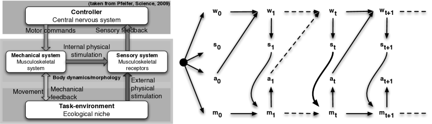
Figure 1: Sensori-motor loop: The figure above shows the sensorimotor loop as a causal Bayesian graph. Right-hand side: The black circle on the left-hand side indicates the initial distribution of world state $W_{0}$, the sensor state $S_{0}$, the action state $A_{0}$ and the memory $M_{0}$ at time $t=0$. The sensor state $S_{t}$ depends only on the current world state $W_{t}$. The memory state $M_{t+1}$ depends on the last memory state $M_{t}$, the previous action $A_{t}$, and the current sensor state $S_{t+1}$. The world state $W_{t+1}$ depends on the previous state $W_{t}$ and on the action $A_{t}$. We do not draw a connection between the action $A_{t}$ and the memory state $M_{t+1}$, because we clearly distinguish between inputs and outputs of the memory $M_{t}$ (which is equivalent to the controller). Any input is given by a sensor state $S_{t}$, and any output is given in form of the action state $A_{t}$. The system may not monitor its outputs $A_{t}$ directly, but through a sensor, hence the sensor state $S_{t+1}$. This is consistent with the figure on the left hand side, taken from (Pfeifer ., 2007)

In a first step, we reduce the complexity by looking at reactive controllers, i.e. we omit the explicit memory $M$. We call it explicit memory, to distinguish it from the implicit memory that is given by the adaptation of the policy due to the sensor history. Actions $A_{t}$ are now generated as a result of the current sensor values $S_{t}$. In this reduced Bayesian graph (see Fig. 2A), the notation is changed for readability. The past is denoted by plain letters ($A,S,W$), and the future by primed letters ($S^{\prime},W^{\prime}$). Excluding $M$ from Figure 1, it is qualitatively equivalent to Figure 2A.

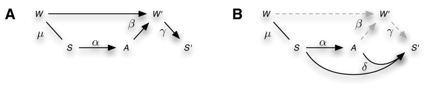
Figure 2: A: This graph shows a reduced version of Figure 1. It shows the progression from one time step $t$ to $t+1$, but with different labeling to highlight the section of the graph which is of interest here. The random variables $A,W,S$ denote the present, given by some distribution $\mu$, while $W^{\prime},S^{\prime}$ denote the future. The kernel $\alpha(a|s)$ defines the policy, i.e. which action $a$ will be chosen, if the sensor state $s$ is seen. Similarly, the kernels $\beta(w^{\prime}|w,a)$ and $\gamma(s|w)$ denote the evolution of the world in dependence of the action and last world state ($\beta$) and the effect of the world on the sensor state ($\gamma$). B: This graph shows how a learning rule is derived from this Bayesian network. As $\beta$ and $\gamma$ are not available to the system, it has to build an internal world model $\delta(s^{\prime}|a,s)$ to compensate for $\beta$ and $\gamma$.

Before the derivation of the learning rule can be discussed, we need to give the basic notations of entropy and mutual information. The entropy $H(X)$ of a random variable $X$, measuring its uncertainty, is defined as:

$$H(X)=-\sum_{x\in\mathcal{X}}p(x)\log p(x).$$ (1)

All calculations in this work are given with respect to the base two logarithm $\log_{2}$. The mutual information of two random variables $X$ and $Y$ is used in this paper in the following form:

$$I(X;Y)=H(X)-H(X|Y).$$ (2)

It measures how much the knowledge of $Y$ reduces the uncertainty of $X$, and it is symmetric, i.e. $I(X;Y)=I(Y;X)$ (Cover  Thomas, 2006). The upper bounds of the entropy and the mutual information are needed later in this work. The maximal entropy is the entropy of a uniform distribution and is, in this case, given by $H(X)\leq\log_{2}|\mathcal{X}|$. The equation (see eq. 2) shows that the mutual information is naturally bounded by the entropy $H(X)$.

We can now define quantities of interest within the resulting compact causal Bayesian network. The mutual information of past and future sensor values, known as the predictive information (Bialek ., 2001), has been shown to be the most natural complexity measure for time series <see¿[for a discussion]Bertschinger2008An-information-theoretic. It is also known as excess entropy (Crutchfield  Young, 1989) and effective measure complexity (Grassberger, 1986), and plays an important role in the related work of e.g. Still (2009) on interactive learning.

Predictive information is defined as $I(S_{p};S_{f})$, where $S_{p}=(\ldots,S_{-2},S_{-1},S_{0})$ is the past, and $S_{f}=(S_{1},S_{2},S_{3},\ldots)$ is the future of all sensor states with respect to the current time step $t=0$. It can also be understood in terms of entropies as the reduction of the uncertainty of the future, given the past.

It is impossible to sample the entire past and future of a system in any concrete implementation. Therefore, we use a first order approximation of the predictive information, i.e. the mutual information of two consecutive sensor values $I(S_{t+1};S_{t})$, denoted by $I(S^{\prime};S)$, as the quantity of interest here. It will not come close to the actual predictive information $I(S_{p};S_{f})$ as any embedded system, in general, is far from being a Markov’ian system, i.e. a system in which the current state only depends on the previous state. Nevertheless, the applicability of this approximation has been shown in previous work (Ay ., 2008; Der ., 2008). To increase the readability, the term predictive information is used instead of approximated predictive information in the remainder of this work, but we always refer to $I(S^{\prime};S)$ instead of $I(S_{p};S_{f})$ and we use the abbreviation PI for it. The goal of this work can now be reformulated using this terminology. We are looking for a learning rule that maximizes the predictive information $I(S^{\prime};S)$ by modifying the policy $\alpha(a|s)$.

The calculation of the PI relies on knowledge about the progression of the world, i.e. knowledge about the kernels $\beta(w^{\prime}|w,a)$ and $\gamma(s^{\prime}|w^{\prime})$. These kernels are not accessible to the system, as a cognitive system can only rely on information that is intrinsically available. To solve this problem, we introduce an intrinsic world model $\delta(s^{\prime}|a,s)$ to replace $\beta$ and $\gamma$ (see Fig. 2B). This replacement is valid, as the joint probability distribution $p(s^{\prime},s)$ is sufficient to calculate $I(S^{\prime};S)$:

$$I(S^{\prime};S) =\sum_{s^{\prime},s\in\mathcal{S}}p(s^{\prime},s)\log_{2}\frac{p(s^{\prime},s)}{p(s^{\prime})p(s)}, p(s) =\sum_{s^{\prime}\in\mathcal{S}}p(s^{\prime},s), p(s^{\prime})=\sum_{s\in\mathcal{S}}p(s^{\prime},s),$$ (3)

and we can deduce from Figure 2B that:

$$p(s^{\prime},s) =\sum_{a\in\mathcal{A}}p(s,a,s^{\prime})=\sum_{a\in\mathcal{A}}p(s)\alpha(a|s)\delta(s^{\prime}|s,a).$$ (4)

This shows that the predictive information $I(S^{\prime};S)$ can be calculated without $\beta$ and $\gamma$ if the sensor distribution $p(s)$, the policy $\alpha(a|s)$ and the intrinsic world model $\delta(s^{\prime}|s,a)$ are known. This intrinsically calculated PI converges to the actual PI (for a stationary process) as the sampled intrinsic world model $\delta(s^{\prime}|s,a)$ converges against the actual world model. As will be shown later, this is the case in the experiments presented in this work (see Sec. 3).

Now, the natural gradient (Amari, 1998) of the predictive information can be calculated with respect to the policy $\alpha(a|s)$ (see app. A for details). In a first step, we represent the distributions $p(s)$, $\alpha(a|s)$, and $\delta(s^{\prime}|s,a)$ as matrices. This explicitly means, that we do not restrict the possible probability distributions and models. Next, the update equations for the sensor distribution, the world model and the policy are given.

The sensor distribution is simply sampled over time and it is given by:

$$p^{(0)}(s) :=\frac{1}{|\mathcal{S}|}$$

$$p^{(n)}(s) :=\left\{\begin{array}[]{cl}\displaystyle\frac{n}{n+1}p^{(n-1)}(s)+\frac{1}{n+1}&\text{if }S_{n+1}=s\\[21.52771pt] \displaystyle\frac{n}{n+1}p^{(n-1)}(s)&\text{if }S_{n+1}\not=s\end{array}\right.$$ (7)

The update rule for the world model is very similar to the rule for the updating of the sensor distribution and reads:

$$\delta^{(0)}(s^{\prime}|s,{a}) :=\frac{1}{|S|}$$

$$\delta^{\left(n_{a}^{s}\right)}(s^{\prime}|s,{a}) :=\left\{\begin{array}[]{ll}\displaystyle\frac{n_{a}^{s}}{n_{a}^{s}+1}\delta^{(n_{a}^{s}-1)}(s^{\prime}|s,{a})+\frac{1}{n_{a}^{s}+1}&{{\text{if }{S_{n_{a}^{s}+1}=s^{\prime},\,S_{n}=s,\,A_{n_{a}^{s}+1}={a}}}}\\[12.91663pt] \displaystyle\frac{n_{a}^{s}}{n_{a}^{s}+1}\delta^{(n_{a}^{s}-1)}(s^{\prime}|s,a)&{\text{if }S_{n_{a}^{s}+1}\not=s^{\prime},\,S_{n}=s,\,A_{n_{a}^{s}+1}={a}}\\[12.91663pt] \delta^{(n_{a}^{s}-1)}(s^{\prime}|s,{a})&{\text{if }S_{n_{a}^{s}}\not=s\text{ or }\,A_{n_{{}_{s,{a}}}+1}\not={a}}\end{array}\right.$$ (11)

What is important to note here is that there is a counter $n_{a}^{s}=1,2,\ldots$ for every pairing of $(s,a)$ to assure that the learning rate for each row of the world model matrix, i.e. each pairing of $(s,a)$, decays according to the number of samples in that row, and not faster. The update rule for the policy (see below) seems complex due to the fact that there are no a priori assumptions about the probability distribution. Using the natural gradient on the predictive information, we get:

$$\alpha^{(0)}({a}|s) :=\frac{1}{|S|}$$

$$\alpha^{(n)}({a}|s) =\alpha^{(n-1)}({a}|s)+\frac{1}{n+1}\alpha^{(n)}({a}|s)\left(F(s)-\sum_{a}\alpha^{(n-1)}(a|s)F(s)\right)$$ (12)

$$F(s) :=p^{(n)}(s)\sum_{s^{\prime}}\delta^{(n)}(s^{\prime}|s,{a})\log_{2}\frac{\sum_{{a}}\alpha^{(n-1)}({a}|s)\delta^{(n)}(s^{\prime}|s,{a})}{\sum_{s^{\prime\prime}}p^{(n)}(s^{\prime\prime})\sum_{a}\alpha^{(n-1)}(a|s^{\prime\prime})\,\delta^{(n)}(s^{\prime}|s^{\prime\prime},a)}$$

Note that our learning rate $\frac{1}{n+1}$ satisfies the standard condition for corresponding rates in stochastic approximation theory, that is $\sum_{n=1}^{\infty}a_{n}^{2}<\infty$, $\sum_{n=1}^{\infty}a_{n}=\infty$ (Benveniste ., 1990). These assumptions are usually made in order to ensure convergence. However, a possible point of criticism here is that the learning and update factors $\frac{1}{n_{a}^{s}+1}$ and $\frac{n_{s}^{a}}{n_{a}^{s}+1}$ are not well chosen, as they lead to strong changes during the first iterations and because they may converge too fast towards zero. Other adaptation factors were evaluated, and are discussed later in this paper (see Sec. 4).

Now that the learning rule is defined, the next step is to evaluate its effect on the PI and the behavior of a system in the sensorimotor loop. This is discussed in the next section.

3 Experiments

The experiments chosen for presentation here are inspired by the previous work of Ay . (2008) and Der . (2008). In the former publication, individually controlled, simple two-wheeled differential drive robots were physically coupled to form a chain which operates in a bounded, featureless environment, while in the latter, a single robot was placed in a bounded environment with cubical obstacles.

In both publications, the predictive information is used in the context of the sensorimotor loop. In (Der ., 2008) a robot chain of length five is equipped with simple parametrized controllers. For each parameter setting, a series of experiments were performed, and the predictive information was then calculated based on the recorded time series. It is shown, that the predictive information is high for parameter settings which also show a high coordination among the robots. The coordination among the robots is measured indirectly by the entropy over the probability distribution of the position of the center robot in the bounded environment. This form of indirect measure of the coordination is also used in this work, but in contrast, this work will also analyze the effect of modifications to the robot chain length on the predictive information and the coordination among the robots.

The work by Ay . (2008) presents a learning rule that maximizes the predictive information under certain constraints. One of the constraints is that the world model $\delta(s^{\prime}|s,a)$ is modeled by a deterministic function with additive Gaussian noise. The result is a learning rule that is equivalent to the Homeokinetic principle by Der (2001); Der  Liebscher (2002).

In summary, this work differs from the previous work in two aspects. First, a learning rule, which is unrestricted with respect to the underlying model and free of assumptions on the world $W_{t}$ is derived and evaluated. Second, the contribution of the chain length to the PI is also analyzed.

3.1 Experimental Setup

The remainder of this section presents the setup of the simulator, the robot, the controller, and finally of the environment, before the following section discusses the results of the experiments.

Simulator:

All experiments were conducted purely in simulation for the sake of simplicity, speed and analysis. It is faster to setup and conduct experiments in simulation, with respect to experiments with real robots, as well as to generate and record the data necessary for analysis. Current simulators, such as YARS (Zahedi ., 2008), which was chosen in this work, are shown to be realistic enough to simulate the relevant physical properties of mobile robots, and designed such that experimental runs can be automated, run at faster than real-time speed, and require minimum effort to setup.

Robots:

In the following paragraphs, we will talk of a chain of identical robots (or chain for short), and thereby mean any number of physically coupled robots including a single robot. A robot in this chain is derived from the Khepera I robot (Mondada ., 1993), which is a two-wheeled differential drive robot with a circular body (see Fig. 3).

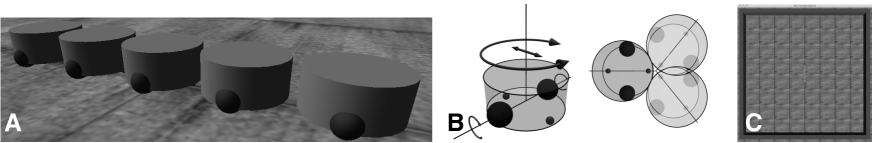
Figure 3: Experimental setup: Figure (B) shows a sketch of the two-wheeled differential drive robot and the connection between neighboring robots, Figure (A) a chain of five robots and Figure (C) and the bounded, featureless environment used in the YARS simulator.

In the experiments presented here, the only inputs and outputs of the robot are its desired wheel velocity ($A_{t}$), and the current actual wheel velocity ($S_{t}$). Both quantities are mapped linearly to the interval of $[-1,1]$, where $-1$ refers to the maximal negative speed (backwards motion), and $+1$ to the maximal positive speed (forward motion). No noise is artificially added to the motors or sensors.

The robots are connected by a limited hinge joint with a maximal deviation of $\pm 0.9$ rad ($\approx 100$ degree), thereby avoiding intersection of neighboring robots (see Fig. 3).

Three different kinds of experiments are presented in the following section, single robot, three-, and five-segment chains. Chains of two and four robots were also tested, but not chosen for presentation here, as their analysis did not provide additional insights.

Controller:

Inspired by Ay . (2008) and Der . (2008), each robot is controlled locally, i.e. there is no global control which has access to every wheel of every segment. For the local control, two control paradigms are evaluated; combined and split control (see Fig. 4). The former refers to a single controller for both wheels, while in the latter case each wheel has its own controller. There is no communication between the controllers. Any interaction occurs solely through the world $W_{t}$, and hence, through the sensor states $S_{t}$, which are in this case only the current actual wheel velocity. The controllers run at 10Hz. Every experiment was setup to run for $10^{6}$ controller updates, resulting in an overall time for each run of approximately 27.5 simulated hours.

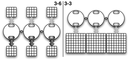
Figure 4: Controller Setup. The labels 3–3 and 3–6 refer to three robots with three controllers, and three robots with six controllers, respectively. Left-hand side: Split controller setup. Each wheel of each robot has an individual controller, i.e. policy matrix $\alpha(a|s)$. Right-hand side: Combined controller setup. Each robot has an individual controller, i.e. policy matrix $\alpha(a|s)$. If the policy matrix $\alpha$ has the size $n\times n$ in the split case, the policy matrix in the combined case has the size $n^{2}\times n^{2}$. For the sake of conciseness, the latter is indicated by a matrix of size $2n\times 2n$, not $n^{2}\times n^{2}$.

In the work presented here, due to the discretisation and matrix representation, pre- and post-processing in the form of binning is required. We chose four equally distributed bins in the interval $[-1,1]$ for the input and output spaces. Different numbers of bins, from 3 to 30, were evaluated. While three bins were dismissed because the result was too close to defining three disjunct actions (forward, stop, backwards), a higher number of bins ($>8$) resulted in less coordination among the robots (compared to four bins).

For the remainder of this work, the notation $r$–$c$ is used, where $r\in\{1,3,5\}$ defines the number of robots, and $c\in\{r,2r\}$ gives the number of controllers. Therefore, the label 1-1 refers to a single robot with a single controller for both wheels, and, at the other end, 5–10 refers to a chain of five robots, with ten controllers, i.e. one for each wheel (see Fig. 4).

Environment:

The environment is a bounded, but otherwise featureless, chosen large enough for the chains to be able to learn a coordinated behavior. Each of the robots has a size of $10cm$ in diameter. The environment’s size is eight by eight meters. Every chain was started with its center robot in the center of the environment, and with the same initial heading.

4 Results

This section discusses the results from the six experiments presented above. The presentation of the results is given in the following steps. First, it is analyzed if the PI was increased over time for all six configurations, and if so, how close it gets to the theoretical upper bounds. In the next step, the increases of the PI over time are related to modifications of the behavior, answering the question if the maximization of the PI leads to qualitative changes on the behavior. The third step is to quantify the behaviors for comparison. From these findings, a seventh experiment is derived and analyzed, in which a combined controller of the 1–1 configuration is initiated with the two optimal split controllers from the 1–2 configuration.

4.1 Maximizing the Predictive Information

The first step is to analyze and compare the development and the maximally achieved values of the predictive information for the six settings. The Figure 5 shows the progression of the predictive information over the entire time, with embedded plots for the initial learning phase. The tables (Tab. 1) show the final PI values for the six experiments, and PI values calculated as an external observer. How the latter is calculated will be explained later in this section.

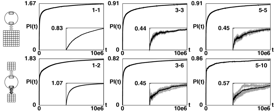
Figure 5: Average-PI plots for each of the six experiments. The ordering from upper left to lower right is, 1–1, 3–3, 5–5, 1–2, 3–6, 5–10. The evolution of the average PI is shown in black in each plot. The embedded small plots show the progress for the first five minutes of each run, including the PI for each controller, plotted in gray.

Final intrinsic PI
c / r	1	3	5
combined	1.66	0.90	0.89
	42%	23%	23%
split	1.80	0.80	0.84
	92%	42%	42%

PI on recorded data
c / r	1	3	5
combined	2.60	1.59	1.70
	27%	16%	17%
split	4.01	2.25	2.39
	41%	23%	24%
(upper bound $\log_{2}(30^{2})\approx 9.81)$

Table 1: Comparison of intrinsically calculated PI (left-hand side) and PI calculated a posteriori on the recoded data per robot (right-hand side). The ordering is roughly kept, but more differentiated, which is also the result of the higher binning (4 vs. 30 bins).

The first result from the Figure 5 is that the learning rule as defined in the equations (7)-(12) successfully increases the PI in all six configurations. To be able to understand how well the PI is maximized, the values are compared to their theoretical upper bounds, which can be calculated from the chosen binning. In the split controller case, the theoretical upper bound is given by $\log_{2}4=2$, while the upper bound for the combined case is given by $\log_{2}16=4$. The comparison of the achieved PI values with their upper bounds is shown in Table 1. The configuration 1–2 almost achieves is maximum, while the configurations 1–1, 3–6, 5–10 are equally successful with about 42% of their maximum. The configurations 3–3 and 5–5 have the smallest relative PI with about 23%.

The results are not well comparable across controller paradigms, as two processes, one with a single channel (split control) and the other with two channels (combined control) are compared. A better way is to compare the PI per robot, and hence, the PI is calculated additionally on the recoded sensor data. This is done in the following way. For each time step, the actual sensor values $S_{l}(t),S_{r}(t)\in[-1,1]$ were recorded and binned into thirty equally distributed bins for each wheel. From this data, the mutual information $I(\{S_{l}(t),S_{r}(t)\};\{S_{l}(t+1),S_{r}(t+1)\})$ is calculated over the last $5\cdot 10^{5}$ points in the data set and the results are shown in Table 1. The results allow a direct comparison of the configurations and the values and show that the chains of length three and five maximize comparably well, although the split controller configurations show slightly higher values. For the single robot configuration, both are significantly higher compared to the multi-robot chains, and again, the split controller outperforms the combined controller with respect to the PI achievement.

At this point, the conclusion is, that the single robots configurations succeed better in maximizing the predictive information compared to longer chains, and that in general split controller outperform the combined counterpart. The next step is to relate these findings with the behaviors of the systems.

4.2 Comparing behaviors

Before the behaviors are analyzed and related to the results of the previous section, we briefly repeat what the predictive information measures. The predictive information ($I(S^{\prime};S)=H(S)-H(S^{\prime}|S)$) is high, if the sensor entropy $H(S)$ is high, and if the uncertainty of the future given the past $H(S^{\prime}|S)$ is low. Applied to the chains, we expect a high predictive information if the controllers have high wheel velocity variance ($H(S)$), but at the same time low variance in the changes of the wheel velocity ($H(S^{\prime}|S)$). This means that each configuration should try to sense every wheel velocity with almost same probability, and at the same time be as deterministic as possible.

The trajectories cannot be visualized entirely, as the resulting plots would not show distinguishable trails. Therefore, the Figure 6 shows the first ten minutes in Grey, and the last 100 minutes in black in the foreground. The Grey trajectory shows the behavior during the initial learning phase, while the black trajectory shows the converged behavior.

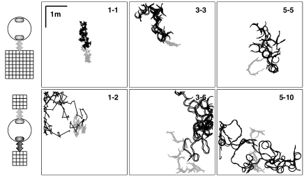
Figure 6: Trajectories: These six plots show the trajectories of the six systems for the first ten minutes (Grey) and the last 100 minutes (black). From upper left to lower right: 1–1, 3–3, 5–5, 1–2, 3–6, 5–10. The plots show that the length of the trails with consecutive movement increases with the number of robots, and with split controllers.

The single robot with split controller (1–2) shows straight and rotational movements. The chains show wavy lines and alternating headings. To better differentiate the behaviors, two quantification methods are used, which are both explained in the following paragraphs.

The first quantification method is the coverage entropy used by Der . (2008). The bounded space is divided into 400 ($20\times 20$) patches of equal size. At every time step, the position of the center robot is measured, and the counter for the corresponding patch is increased. This gives a visit frequency for each patch, from which the coverage entropy is calculated (see Fig. 7, left-hand side). It is plotted over time, as it then shows how fast a system covers the entire space.

The second method is designed to show how the behaviors vary over time. In this second case, the coverage entropy is calculated on a sliding window. For the Figure 7 (right-hand side), a sliding window of width $10^{3}$ was chosen. The resulting $10^{3}$ values are used as control points for a Bézier curve.

Figure 7: Coverage Entropy: Left-hand side: The overall coverage entropy (see text for detailed explanation). The plot shows that every configuration finally covers the entire space (in $T=10^{6}$ time steps). The ranking of the label corresponds to the speed with which the coverage is achieved. Right-hand side: Coverage entropy for a sliding window of ten seconds, plotted as a Bézier curve ($T\approx 10^{6}$ time step). This plot shows that 5–10 is the fastest to achieve a good exploration behavior, followed by 3–6. The configuration 1–2 requires much more time, but eventually shows comparable exploration behavior. The robots with combined control of the wheels are all outperformed by those with split control.

The results of both methods (see Fig. 7) allow the following conclusions:

1. All configurations explore the entire area (see Fig. 7, left-hand side), but require different time.

2. Longer consecutive trails relate to higher average sliding window coverage entropy (compare Fig. 6 with the right-hand side of Fig. 7).

3. The configurations which show longer consecutive trails are those, which reach higher coverage entropy sooner.

As stated earlier, movements only occur for chains with length larger than one if the majority of the segments moves in one direction. Therefore, the sliding window coverage entropy allows us to indirectly measure the cooperation of the segments. We therefore see higher cooperation among the segments of the split configuration, when compared to their combined controller counterparts. This will be discussed at the end of this paper (see Sec. 5).

Obviously, the measures do not relate to cooperation for the single robot configurations, but the measures also show here that higher PI relates to higher coverage entropy and higher sliding window coverage entropy, for the split controller paradigm.

Configuration 1–2 is the only one to achieve almost maximal PI. Therefore, its strategy is chosen for analysis in the next section. In addition, the behavior of the configuration 3–6 is analyzed, as it reveals why longer chains result in longer trails. Furthermore, it shows that the solution for the chains with more than one robot is not binning-specific.

4.3 Behavior Analysis:

For the analysis, each configuration was fixed after learning, and then run for one simulated hour ($3.6\cdot 10^{4}$ iterations) during which the controller output $A$ and the sensory input $S$ was recorded. Figures 9 to 10 are taken from these recordings and show the actions as bars, and the sensor states as lines.

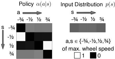
Figure 8: Policy and sensor distributions of the configuration 1–2. The matrices of the left wheel are shown, as the right wheel matrices do not show a significant difference. The matrix on the left-hand side is the policy $\alpha(a|s)$. The columns represent the action, starting from left to right, i.e. the action representing high backward motion $\left(-\frac{3}{4}\right)$ is the left most column, while the action representing high forward motion $\left(\frac{3}{4}\right)$ is the right most column. Similarly, the sensor states are represented by the rows, where the top most row represents full backward motion and the lowest row, full forward motion. The numbers represent the bin centers. The vector on the right-hand side is the sensor or input distribution $p(s)$.

The following naming convention is used in the paragraphs ahead. The bins are named with respect to their center, i.e. $-\frac{3}{4}$, $-\frac{1}{2}$, $\frac{1}{2}$, $\frac{3}{4}$. These names relate to the maximal positive ($-1$) and negative ($+1$) wheel velocities. The policy and sensor distribution configuration is shown exemplarily for the 1–2 configuration in Figure 8.

Configuration 1–2:

The policy and transient plots (see Fig. 9) reveal how the maximal PI is achieved.

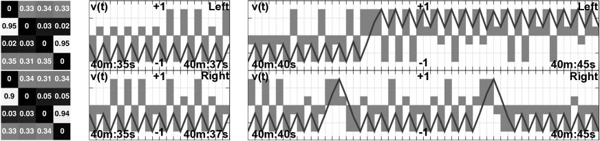
Figure 9: 1–2: Left: Policies for left (upper) and right (lower) wheel. Center: Transient plot for a sequence of straight movement. Right: Transient plot for a sequence of rotations.

The transient plot displaying straight movement (see Fig. 9, center) shows that the wheel velocities oscillate between $-\frac{1}{2}$ and $-\frac{3}{4}$. This oscillation is stable due to the physical properties of the system for the following reason. The sensor state $S=-\frac{3}{4}$ results in an action $A\in\{-\frac{1}{2},\frac{1}{2},\frac{3}{4}\}$. Due to the inertia of the system and the controller frequency, any selected action $A\in\{-\frac{1}{2},\frac{1}{2},\frac{3}{4}\}$ leads to a sensor state $S=-\frac{1}{2}$, as the desired wheel velocity cannot be reached instantaneously. As a consequence, the action $A=-\frac{3}{4}$ is chosen with a probability of $p(A=-\frac{3}{4}|S=-\frac{1}{2})=0.95$, leading to the observable oscillation during the translational movement of the robot (see Fig. 9, center). With a remaining probability of $p(A\not=-\frac{3}{4}|S=-\frac{1}{2})=0.05$, a change of the direction of the wheel velocity occurs, which leads either to a rotation of the system, or inversion of the translational behavior (see Fig. 9, right-hand side). As a result, the sensor entropy $H(S)$ is high (compare with Fig. 8), but at the same time the conditional entropy $H(S^{\prime}|S)$ is low, leading to the observed high PI.

Configuration 3–6

The transient plot (see Fig. 10) clearly shows a difference to the configuration 1–2, as the wheel velocity of one wheel is no longer only influenced by its controller, but also by the actions of the other controllers. To understand the strategy, the policy for $S=-\frac{3}{4}$ must be taken into account ($S=\frac{3}{4}$ is analogous). With a probability of $p(A\in\{-\frac{3}{4},-\frac{1}{2}\}|S=-\frac{3}{4})\approx 0.6$, the current direction of the wheel rotation is maintained (see Fig. 10, left-hand side). As at least two robots, i.e. four related controllers must move into the same direction, for the entire system to progress, the probability of a switch in the direction is approximately $p\approx 0.4^{4}$. If only one controller switches, the sensor state remains (as discussed above), i.e. the direction of the system is unchanged. This explains how the robots coordinate, and why the configuration 5–10 shows longer consecutive trails with very similar policies (not shown).

These analysis also show that the solutions are not specific to the selected four bins configuration. In an incremental way, one can construct policies of higher dimension by splitting of the values of the corresponding cells. An example is a policy with eight bins, which can be constructed from the four bin policies by the following mapping $p_{\{8\,\,bins\}}(a_{i}|s_{j})=\frac{1}{4}p_{\{4\,\,bins\}}(a_{\lfloor i/2\rfloor}|s_{\lfloor j/2\rfloor})$. This indicates a possibility to incrementally increase the dimension of the policies based on adapted lower dimension solution. A different form of incremental optimization in this context, in which combined controllers can be constructed from split solutions, is discussed in the next section.

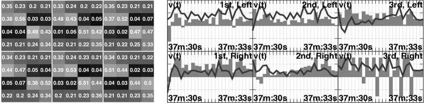
Figure 10: Left-hand side: The 3–6 policy. Right-hand side: Transient plot.

4.4 Incremental Optimization

In the results presented above, the 1–1 configuration was least successful in maximizing its predictive information. In general, the configuration 1–1 should be at least as successful as the 1–2 configuration, because the combined controller has the same capabilities that the system consisting of two split controllers has, if not more. Hence, there are two possible reasons why the 1–1 configuration is less successful. First, it (repeatedly) reaches a sub-optimal solution, and second, the learning and update rate $\frac{1}{n+1}$ has converged faster towards zero than the behavior towards the optimal solution. To exclude the latter possibility, different types of learning rates (bounded below, constant during an initial learning phase, both, and constant) were evaluated, and the experiments clearly showed that the chosen learning rate is not the reason for the sub-optimal solution. To test the former hypothesis, a combined controller was generated from two split controllers, including the initial sensor distribution ($p(s)$) and world model ($\delta(s^{\prime}|s,a)$). The combined policy is generated using the products of the two split policies in the following manner, where the superscripts $l,r,c$ refer to split left, split right and combined controller:

$$\alpha^{l}(a^{l}|s^{l}) =(\alpha^{l}_{s,a}) a =0,1,\ldots,|\mathcal{A}|-1 s =0,1,\ldots,|\mathcal{S}|-1$$

$$\alpha^{r}(a^{r}|s^{r}) =(\alpha^{r}_{s,a})$$

$$\alpha^{c}(a^{c}|s^{c}) =(\alpha^{c}_{s^{c},a^{c}}) a^{c} =0,1,\ldots,|\mathcal{A}|^{2}-1 s^{c} =0,1,\ldots,|\mathcal{S}|^{2}-1$$

$$\alpha^{c}_{s^{c},a^{c}} =\alpha^{l}_{s_{c}^{l},a_{c}^{l}}\cdot\alpha^{r}_{s_{c}^{r},a_{c}^{r}} s_{c}^{l} =s^{c}\mod|\mathcal{S}|,\quad s_{c}^{r}=\left\lfloor\frac{s^{c}}{|\mathcal{S}|}\right\rfloor a_{c}^{l} =a^{c}\mod|\mathcal{A}|,\quad a_{c}^{r}=\left\lfloor\frac{a^{c}}{|\mathcal{A}|}\right\rfloor.$$

The equations above implement cascaded loops, such that the indices for the combined controller $(s^{c},a^{c})=(s^{l}_{c},a^{l}_{c},s^{r}_{c},a^{r}_{c})$ is given by the sequence (shown exemplarily for some elements): $(0,0)=(0,0,0,0)$, $(0,1)=(0,1,0,0)$ $(0,2)=(0,2,0,0)$, …, $(2,10)=(2,2,0,2)$, $(2,11)=(2,3,0,2)$, $(2,12)=(2,0,0,3)$, $(2,13)=(2,1,0,3)$, $(2,14)=(2,2,0,3)$, $(2,15)=(2,3,0,3)$ …

Figure 11A shows the combined controller, composed from the two optimal split controllers of the 1–2 configuration (see Fig. 9). Using this matrix as an initialization for the learning process of the 1–1 configuration leads to the policy shown in Figure 11B. It must be noted that the learning process is now not anymore restricted to the lower dimensional policy space of the split controllers, and therefore, allows for further adjustments. However, it turns out that there is no significant difference between the initial policy A and the converged policy B with respect to the $L^{2}$-norm, which is $d=\sqrt{\sum_{i,j}(a_{ij}-b_{ij})^{2}}=1.9\cdot 10^{-6}$. Consequently, the plots in Figure 12 show that the behavior has also not changed significantly (compare with Fig. 5 [1-2], Fig. 6 [1-2], Fig. 7)

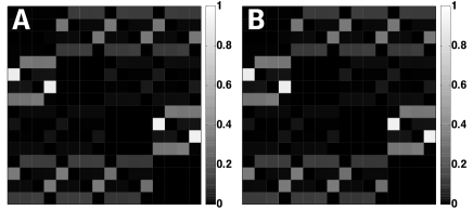
Figure 11: 1–1 Policies. A) Combined policy composed from two split controllers (see text). B) Policy A after $10^{6}$ additional learning iterations.

This is an interesting result, as it shows that the optimal solution in the sub-manifold of the split controllers is also an optimal solution in the space of the combined controllers. A geometric interpretation of this result will follow in the discussion. This shows that a common problem in learning agents, known as bootstrapping (Nolfi  Floreano, 2000), which also occurs here in the case of the 1–1 configuration, can be avoided using the same common strategy of incremental learning for information maximization in the sensorimotor loop.

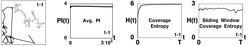
Figure 12: From left to right: Trajectory, predictive information, coverage entropy, sliding window coverage entropy. The plots show that the behavior is unchanged, that the PI is maximal and doubled due to the doubling of the channel capacity, and that the exploration behavior is equivalent to that of the split controller configuration 1–2 (compare with Fig. 5 [1-2], Fig. 6 [1-2], Fig. 7).

To conclude this section, the derived learning rule is able to maximize the predictive information for systems in the sensorimotor loop. Additionally, increases of the PI relate to changes in the behavior and here to a higher coverage entropy, an indirect measure for coordination among the coupled robots.

5 Discussion

This work presented a novel approach to self-organized learning in the sensorimotor loop, which is free of assumptions on the world and restrictions on the model. A learning algorithm was derived from the principle of maximizing the (approximated) predictive information. Following the embodied artificial intelligence approach, the learning rule was tested in experiments with simulated robot chains. As desired, the average approximated predictive information increased over time in each of the presented settings, which was the primary goal of this work.

An important point here is that the increase of the average predictive information alone does not allow conclusions to be drawn about specific changes of the robots behaviors. It is vital to relate the predictive information values to observations of the behaviors of the systems while they interact in their environment, as it is the embodiment, which determines the behavioral changes. This is an essential statement of embodied artificial intelligence, and the reason why we chose robot experiments to evaluate the learning rule.

The second result of this work is especially interesting because it is counterintuitive. The experiments show that there is a higher coverage entropy, a measure for coordinated behavior in this setting, for chain configurations with more robots and as well as such with split controllers. For three reasons this result is counterintuitive; 1) each robot cannot measure the actions of the other robots in the chain directly, but only through its wheel velocity sensor(s), 2) more robots mean that there is more disturbance in the motor-sensor coupling, due to the higher physical interactions, which are a direct result of the number of robots, and 3) the smaller controller setting can only read one sensor and has fewer internal states, which makes it less capable of compensating for the higher disturbances.

We believe that the reason why less complex controllers coordinate better in this setup can be well discussed in the context of morphological computation (Pfeifer  Bongard, 2006), but at this point we propose an information-geometric approach. The set of split policies clearly forms a low-dimensional subfamily of the family of all policies. Therefore, policies with maximal predictive information should be reachable in that larger set. One would even expect that the optimization in the set of split controllers is too restrictive. However, the simulation results suggest that the split controllers have a distinguished geometric property with regard to predictive information. It seems that they constrain the optimization process in such a way that the convergence towards a sub-optimal value of the predictive information becomes unlikely. There is a huge number of local but not global maximizers with moderate predictive information which are avoided through the constraints given by split controllers. Furthermore, the policies that are reached by our learning rule in most cases have a very high predictive information value. In summary, bad policies are excluded and good policies are included through the particular geometry of the family of split controllers. The geometric picture that we sketched here, although not verified analytically, identifies selection criteria for models (families of policies) in artificial learning systems based on the maximization of objective functions such as predictive information.

Appendix

Appendix A Derivation of the learning rule

In order to derive a learning rule for the maximization of predictive information we use the natural gradient method (Amari, 1998), which is based on the Fisher metric. The application of this method to the policy context, within reinforcement learning, has already been introduced by (Peters ., 2005; Kakade, 2002). In our case, where the optimization domain, i.e. the set of all policies, is given in terms of the particular “coordinate system,” the gradient equations with respect to the Fisher metric have the simple structure of replicator equations Hofbauer  Sigmund (2003). Being more precise, we denote by ${\mathcal{P}}({\mathcal{X}})$ the set of strictly positive probability distributions on a non-empty finite set ${\mathcal{X}}$ and consider a differentiable function $F:{\mathcal{P}}({\mathcal{X}})\to\mathbb{R}$. With the gradient $\mathsf{grad}_{p}F$ of that function with respect to the Fisher metric, which is also known as Shahshahani metric, the following replicator equations are obtained (see also theorem 19.5.1 in (Hofbauer  Sigmund, 2003)):

$$\dot{p}(x)\;=\;\mathsf{grad}_{p}F(x)\;=\;p(x)\left(\partial_{x}F(p)-\sum_{x^{\prime}\in{\mathcal{X}}}p(x^{\prime})\,\partial_{x^{\prime}}F(p)\right),\qquad x\in{\mathcal{X}}.$$

The right-hand side of the replicator equation is the gradient that we need for the time discrete gradient ascent. (Here we use $\partial_{x}F$ as the abbreviation for the partial derivative $\frac{\partial F}{\partial p(x)}$.) This gives us the update rule

$$p^{(n+1)}(x)\;=\;p^{(n)}(x)+\frac{1}{n+1}\,p^{(n)}(x)\left({\partial_{x}F}(p^{(n)})-\sum_{x^{\prime}}p^{(n)}(x^{\prime})\,{\partial_{x^{\prime}}F}(p^{(n)})\right),\qquad x\in{\mathcal{X}}.$$ (13)

We have chosen the rate $\frac{1}{n+1}$ in line with the general stochastic approximation theory, where a typical assumption for the learn rates $a_{n}$ is $\sum_{n=1}^{\infty}a_{n}=\infty$, $\sum_{n=1}^{\infty}a^{2}_{n}<\infty$ (Benveniste ., 1990). Now, after having outlined the general procedure, we come to the actual problem of maximizing predictive information. For each sensor value $s$ we consider as the optimization domain, the space of policies $\alpha(a|s)$ which consists of probability distributions on the set of actuator values. As derivative of the mutual information $I(S^{\prime};S)$ with respect to the policy $\alpha(a|s)$ we have:

$$\frac{\partial I(S^{\prime};S)}{\partial\alpha(a|s)} =p(s)\sum_{s^{\prime}}\delta(s^{\prime}|s,a)\ln\frac{\sum_{a}\alpha(a|s)\,\delta(s^{\prime}|s,a)}{\sum_{s^{\prime\prime}}p(s^{\prime\prime})\sum_{a}\alpha(a|s^{\prime\prime})\,\delta(s^{\prime}|s^{\prime\prime},a)}$$ (14)

Note that there is an implicit dependence of the stationary distribution $p(s)$ on the policy $\alpha(a|s)$ which complicates the derivative. This dependence is not considered here, as it is subject of current research.

Together with the general iteration rule (13) the derivative (14) results in a corresponding iteration rule for the mutual information which almost coincides with rule (12). In order to obtain the final step, note that the mutual information with respect to the kernel $\delta(s^{\prime}|s,a)$ is not necessarily consistent with the actual mutual information generated through the mechanisms of the world. Therefore, we adjust $\delta(s^{\prime}|s,a)$ to the empirical data according to our rule (11). The resulting sequence $\delta^{(n)}(s^{\prime}|s,a)$ is then used for iteration (13).

Acknowledgments

We thank the anonymous referees for the constructive comments and Daniel Polani for the many fruitful discussions.

References

- Amari (\APACyear1998) \APACinsertmetastarAmari1998Natural-Gradient-WorksAmari, S. \BBOP1998\BBCP. \BBOQNatural gradient works efficiently in learning.\BBCQ \BemNeural Computation, \Bem10(2), 251-276.
- Ay \BOthers. (\APACyear2008) \APACinsertmetastarAy2008Predictive-information-andAy, N., Bertschinger, N., Der, R., Güttler, F.\BCBL \BBA Olbrich, E. \BBOP2008\BBCP. \BBOQPredictive information and explorative behavior of autonomous robots.\BBCQ \BemThe European Physical Journal B - Condensed Matter and Complex Systems, \Bem63(3), 329–339.
- Barto (\APACyear2004) \APACinsertmetastarBarto2004Intrinsically-motivated-learningBarto, A. G. \BBOP2004\BBCP. \BBOQIntrinsically motivated learning of hierarchical collections of skills.\BBCQ \BIn \BemProceedings of 3rd int. conference development learn. (\BPGS 112–119). San Diego, CA, USA.
- Benveniste \BOthers. (\APACyear1990) \APACinsertmetastarBenveniste1990Adaptive-algorithms-andBenveniste, A., Priouret, P.\BCBL \BBA Métivier, M. \BBOP1990\BBCP. \BemAdaptive algorithms and stochastic approximations. New York, NY, USA: Springer-Verlag New York, Inc.
- Bertschinger (\APACyear2008) \APACinsertmetastarBertschinger2008An-information-theoreticBertschinger, N. \BBOP2008\BBCP. \BemAn information theoretic perspective on cognitive systems: Memory and autonomy. \BPhD, Univeristy of Leipzig.
- Bialek \BOthers. (\APACyear2001) \APACinsertmetastarBialek2001Predictability-Complexity-andBialek, W., Nemenman, I.\BCBL \BBA Tishby, N. \BBOP2001\BBCP. \BBOQPredictability, complexity, and learning.\BBCQ \BemNeural Computation, \Bem13(11), 2409–2463.
- Brooks (\APACyear1986) \APACinsertmetastarBrooks1986A-Robust-LayeredBrooks, R. A. \BBOP1986, March\BBCP. \BBOQA robust layered control system for a mobile robot.\BBCQ \BemIEEE Journal of Robotics and Automation, \Bem2(1), 14–23.
- Brooks (\APACyear1991) \APACinsertmetastarBrooks1991Intelligence-Without-ReasonBrooks, R. A. \BBOP1991\BBCP. \BBOQIntelligence without reason.\BBCQ \BIn J. Myopoulos \BBA R. Reiter (\BEDS), \BemProceedings of the 12th international joint conference on artificial intelligence (IJCAI-91) (\BPGS 569–595). Sydney, Australia: Morgan Kaufmann publishers Inc.: San Mateo, CA, USA.
- Clark (\APACyear1996) \APACinsertmetastarClark1996Being-There:-PuttingClark, A. \BBOP1996\BBCP. \BemBeing there: Putting brain, body, and world together again. Cambridge, MA, USA: MIT Press.
- Cliff (\APACyear1990) \APACinsertmetastarCliff1990Computational-neuroethology:-aCliff, D. \BBOP1990\BBCP. \BBOQComputational neuroethology: a provisional manifesto.\BBCQ \BIn \BemProceedings of the first international conference on simulation of adaptive behavior on from animals to animats (\BPGS 29–39). Cambridge, MA, USA: MIT Press.
- Cover \BBA Thomas (\APACyear2006) \APACinsertmetastarCover2006Elements-of-InformationCover, T. M.\BCBT \BBA Thomas, J. A. \BBOP2006\BBCP. \BemElements of information theory (2nd, \BED). Wiley.
- Crutchfield \BBA Young (\APACyear1989) \APACinsertmetastarCrutchfield1989Inferring-statistical-complexityCrutchfield, J. P.\BCBT \BBA Young, K. \BBOP1989, Jul\BBCP. \BBOQInferring statistical complexity.\BBCQ \BemPhys. Rev. Lett., \Bem63(2), 105–108.
- Der (\APACyear2001) \APACinsertmetastarDer2001Self-Organized-Acquisition-ofDer, R. \BBOP2001\BBCP. \BBOQSelf-organized acquisition of situated behavior.\BBCQ \BemTheory in Biosciences, \Bem120, 179-187.
- Der \BOthers. (\APACyear2008) \APACinsertmetastarDer2008Predictive-information-andDer, R., Güttler, F.\BCBL \BBA Ay, N. \BBOP2008\BBCP. \BBOQPredictive information and emergent cooperativity in a chain of mobile robots.\BBCQ \BIn \BemAlifexi proceedings.
- Der \BBA Liebscher (\APACyear2002) \APACinsertmetastarDer2002True-autonomy-fromDer, R.\BCBT \BBA Liebscher, R. \BBOP2002\BBCP. \BBOQTrue autonomy from self-organized adaptivity.\BBCQ \BIn \BemProc. workshop biologically inspired robotics. the legacy of grey walter 14-16 august 2002, bristol labs. Bristol.
- Di Paolo (\APACyear2000) \APACinsertmetastarDi-Paolo2000Homeostatic-adaptation-toDi Paolo, E. A. \BBOP2000\BBCP. \BBOQHomeostatic adaptation to inversion of the visual field and other sensorimotor disruptions.\BBCQ \BIn J.-A. Meyer, A. Berthoz, H. Floreano D. and. Roitblat\BCBL \BBA S. Wilson (\BEDS), \BemFrom animals to animats 6. proceedings of the VI international conference on simulation of adaptive behavior. Cambridge, MA: MIT Press.
- Förster (\APACyear1993) \APACinsertmetastarForster1993Wissen-und-GewissenFörster, H. von. \BBOP1993\BBCP. \BemWissen und Gewissen : Versuch einer Brücke (1. Aufl. \BEd; S. J. Schmidt, \BED). Frankfurt am Main, D: Suhrkamp.
- Grassberger (\APACyear1986) \APACinsertmetastarGrassberger1986Toward-a-quantitativeGrassberger, P. \BBOP1986, 09\BBCP. \BBOQToward a quantitative theory of self-generated complexity.\BBCQ \BemInternational Journal of Theoretical Physics, \Bem25(9), 907–938.
- Hofbauer \BBA Sigmund (\APACyear2003) \APACinsertmetastarHofbauer2003Evolutionary-game-dynamicsHofbauer, J.\BCBT \BBA Sigmund, K. \BBOP2003\BBCP. \BBOQEvolutionary game dynamics.\BBCQ \BemBull. Amer. Math. Soc., \Bem40, 479–519.
- Kakade (\APACyear2002) \APACinsertmetastarKakade2002A-natural-policyKakade, S. \BBOP2002\BBCP. \BBOQA natural policy gradient.\BBCQ \BemAdvances in neural information processing systems, \Bem2, 1531–1538.
- Kaplan \BBA Oudeyer (\APACyear2004) \APACinsertmetastarKaplan2004Maximizing-Learning-Progress:Kaplan, F.\BCBT \BBA Oudeyer, P.-Y. \BBOP2004\BBCP. \BBOQMaximizing learning progress: An internal reward system for development.\BBCQ \BemEmbodied Artificial Intelligence, 629–629.
- Laughlin (\APACyear1981) \APACinsertmetastarLaughlin1981A-simple-codingLaughlin, S. \BBOP1981\BBCP. \BBOQA simple coding procedure enhances a neuron’s information capacity.\BBCQ \BemZ Naturforsch C, \Bem36(9-10), 910-2.
- Linsker (\APACyear1988) \APACinsertmetastarLinsker1988Self-organization-in-aLinsker, R. \BBOP1988\BBCP. \BBOQSelf-organization in a perceptual network.\BBCQ \BemIEEE Computers, \Bem88, 105–117.
- Lungarella \BBA Sporns (\APACyear2005) \APACinsertmetastarLungarella2005Information-Self-Structuring:-KeyLungarella, M.\BCBT \BBA Sporns, O. \BBOP2005\BBCP. \BBOQInformation self-structuring: Key principle for learning and development.\BBCQ \BemDevelopment and Learning, 2005. Proceedings. The 4th International Conference on, 25–30.
- Meltzoff \BBA Moore (\APACyear1997) \APACinsertmetastarMeltzoff1997Explaining-facial-imitation:Meltzoff, A.\BCBT \BBA Moore, M. K. \BBOP1997\BBCP. \BBOQExplaining facial imitation: A theoretical model.\BBCQ \BemEarly Development and Parenting, 179–192.
- Mondada \BOthers. (\APACyear1993) \APACinsertmetastarMondada1993Mobile-Robot-Miniaturization:Mondada, F., Franzi, E.\BCBL \BBA Ienne, P. \BBOP1993\BBCP. \BBOQMobile robot miniaturization: A tool for investigation in control algorithms.\BBCQ \BIn \BemProceedings of the third international symposium on experimental robotics (\BPGS 501–513). Berlin: Springer Verlag.
- Nolfi \BBA Floreano (\APACyear2000) \APACinsertmetastarNolfi2000Evolutionary-RoboticsNolfi, S.\BCBT \BBA Floreano, D. \BBOP2000\BBCP. \BemEvolutionary robotics. MIT Press.
- Oudeyer \BOthers. (\APACyear2007) \APACinsertmetastarOudeyer2007Intrinsic-Motivation-SystemsOudeyer, P.-Y., Kaplan, F.\BCBL \BBA Hafner, V. \BBOP2007, April\BBCP. \BBOQIntrinsic motivation systems for autonomous mental development.\BBCQ \BemEvolutionary Computation, IEEE Transactions on, \Bem11(2), 265-286.
- Pasemann \BOthers. (\APACyear2004) \APACinsertmetastarPasemann2004Adaptive-Behaviour-ControlPasemann, F., Zahedi, K.\BCBL \BBA Rohde, M. \BBOP2004\BBCP. \BemAdaptive behaviour control by self-regulating neurons (Preprint \BNUM 55). MPI MiS.
- Peters \BOthers. (\APACyear2005) \APACinsertmetastarPeters2005natural-actor-criticPeters, J., Vijayakumar, S.\BCBL \BBA Schaal, S. \BBOP2005\BBCP. \BBOQNatural actor-critic.\BBCQ \BIn \Bemproceedings of the 16th european conference on machine learning (ecml 2005) (\BPG 280-291). springer.
- Pfeifer \BBA Bongard (\APACyear2006) \APACinsertmetastarPfeifer2006How-the-BodyPfeifer, R.\BCBT \BBA Bongard, J. C. \BBOP2006\BBCP. \BemHow the body shapes the way we think: A new view of intelligence. The MIT Press (Bradford Books).
- Pfeifer \BOthers. (\APACyear2007) \APACinsertmetastarPfeifer2007Self-Organization-Embodiment-andPfeifer, R., Lungarella, M.\BCBL \BBA Iida, F. \BBOP2007\BBCP. \BBOQSelf-organization, embodiment, and biologically inspired robotics.\BBCQ \BemScience, \Bem318(5853), 1088–1093.
- Polani \BOthers. (\APACyear2006) \APACinsertmetastarPolani2006Relevant-Information-inPolani, D., Nehaniv, C., Martinetz, T.\BCBL \BBA Kim, J. T. \BBOP2006\BBCP. \BBOQRelevant Information in Optimized Persistence vs. Progeny Strategies.\BBCQ \BIn L. M.Rocha, M. Bedau, D. Floreano, R. Goldstone, A. Vespignani\BCBL \BBA L. Yaeger (\BEDS), \BemProc. artificial life x.
- Porr (\APACyear2003) \APACinsertmetastarPorr2003Sequence-Learning-in-aPorr, B. \BBOP2003\BBCP. \BemSequence-learning in a self-referential closed-loop behavioural system. \BPhD, Faculty of Human Sciences, Department of Psychology.
- Schmidhuber (\APACyear1990) \APACinsertmetastarSchmidhuber1990A-possibility-forSchmidhuber, J. \BBOP1990\BBCP. \BBOQA possibility for implementing curiosity and boredom in model-building neural controllers.\BBCQ \BIn \BemProceedings of the first international conference on simulation of adaptive behavior on from animals to animats (\BPGS 222–227). Cambridge, MA, USA: MIT Press.
- Schmidhuber (\APACyear2009) \APACinsertmetastarSchmidhuber2009Driven-by-CompressionSchmidhuber, J. \BBOP2009\BBCP. \BBOQDriven by compression progress: A simple principle explains essential aspects of subjective beauty, novelty, surprise, interestingness, attention, curiosity, creativity, art, science, music, jokes.\BBCQ \BemAnticipatory Behavior in Adaptive Learning Systems, 48–76.
- Shannon (\APACyear1948) \APACinsertmetastarShannon1948A-mathematical-theoryShannon, C. E. \BBOP1948\BBCP. \BBOQA mathematical theory of communication.\BBCQ \BemBell System Technical Journal, \Bem27, 379—423.
- Steels (\APACyear2004) \APACinsertmetastarSteels2004The-Autotelic-PrincipleSteels, L. \BBOP2004\BBCP. \BBOQThe autotelic principle.\BBCQ \BemEmbodied Artificial Intelligence, 629–629.
- Steels \BBA Wellens (\APACyear2007) \APACinsertmetastarSteels2007Scaffolding-Language-EmergenceSteels, L.\BCBT \BBA Wellens, P. \BBOP2007\BBCP. \BBOQScaffolding language emergence using the autotelic principle.\BBCQ \BIn \BemIeee symposium on artificial life (\BPG 325-332).
- Still (\APACyear2009) \APACinsertmetastarStill2009Information-theoretic-approach-toStill, S. \BBOP2009, jan\BBCP. \BBOQInformation-theoretic approach to interactive learning.\BBCQ \BemEPL, \Bem85(2), 28005.
- Storck \BOthers. (\APACyear1995) \APACinsertmetastarStorck1995Reinforcement-Driven-InformationStorck, J., Hochreiter, S.\BCBL \BBA Schmidhuber, J. \BBOP1995\BBCP. \BBOQReinforcement driven information acquisition in non-deterministic environments.\BBCQ \BIn \BemProceedings of the international conference on artificial neural networks (\BPGS 159–164).
- Thelen \BBA Smith (\APACyear1996) \APACinsertmetastarThelen1996A-dynamic-systemsThelen, E.\BCBT \BBA Smith, L. B. \BBOP1996\BBCP. \BemA dynamic systems approach to the development of cognition and action. Cambridge, Mass. u.a.: MIT Press.
- Uexkuell (\APACyear1957 [1934]) \APACinsertmetastarUexkuell1957A-Stroll-ThroughUexkuell, J. von. \BBOP1957 [1934]\BBCP. \BBOQA stroll through the worlds of animals and men.\BBCQ \BIn C. H. Schiller (\BED), \BemInstinctive behavior (\BPG 5-80). New York: International Universities Press.
- Williams \BBA Kelley (\APACyear2009) \APACinsertmetastarWilliams2009gnuplot-4.2.6Williams, T.\BCBT \BBA Kelley, C. \BBOP2009, September\BBCP. \Bemgnuplot 4.2.6. http://www.gnuplot.info.
- Zahedi \BOthers. (\APACyear2008) \APACinsertmetastarZahedi2008YARS:-A-PhysicalZahedi, K., Twickel, A. von\BCBL \BBA Pasemann, F. \BBOP2008\BBCP. \BBOQYars: A physical 3d simulator for evolving controllers for real robots.\BBCQ \BIn S. Carpin \BBA et al. (\BEDS), \BemSimpar 2008 (\BPGS 71—82). Springer.