Strategies for online inference of model-based clustering in large and growing networks

Abstract

In this paper we adapt online estimation strategies to perform model-based clustering on large networks. Our work focuses on two algorithms, the first based on the SAEM algorithm, and the second on variational methods. These two strategies are compared with existing approaches on simulated and real data. We use the method to decipher the connexion structure of the political websphere during the US political campaign in 2008. We show that our online EM-based algorithms offer a good trade-off between precision and speed, when estimating parameters for mixture distributions in the context of random graphs.

T1Supported in part by French Agence Nationale de la Recherche Grant NeMo ANR-08-BLAN-0304-01.

, ,
and

1 Introduction

Analyzing networks has become an essential part of a number of scientific fields. Examples include such widely differing phenomena as power grids, protein-protein interaction networks and friendship. In this work we focus on particular networks which are made of political Weblogs. With the impact of new social network websites like Myspace and Facebook, the web has an increasing influence on the political debate. As an example, Adamic and Glance (2005) showed that blogging played an important role in the political debate of the 2004 US Presidential Election. Although only a small minority of Americans actually used these Weblogs, their influence extended far beyond their readership, as a result of their interactions with national mainstream media. In this article we propose to uncover the connexion structure of the political websphere during the US political campaign in 2008. This data set consists of a one-day snapshot of over 130,520 links and 1870 manually classified websites (676 liberal, 1026 conservative and 168 independent) where nodes are connected if there exists a citation from one to another.

Many strategies have been developed to study networks structure and topology. A distinction can be made between model-free [Newman (2006); Ng, Jordan and Weiss (2002)] and model-based methods, with connexions between parametric and nonparametric models [Bickel and Chen (2009)]. Among model-based methods, model-based clustering has provided an efficient way to summarize complex networks structures. The basic idea of these strategies is to model the distribution of connections in the network, considering that nodes are spread among an unknown number of connectivity classes which are themselves unknown. This generalizes model-based clustering to network data, and various modeling strategies have been considered. Nowicki and Snijders (2001) propose a mixture model on dyads that belong to some relational alphabet, Daudin, Picard and Robin (2008) propose a mixture on edges, Handcock, Raftery and Tantrum (2007) consider continuous hidden variables and Airoldi et al. (2005, 2007, 2008) consider both mixed membership and stochastic block structure.

In this article our concern is not to assess nor to compare the appropriateness of these different models, but we focus on a computational issue that is shared by most of them. Indeed, even if the modeling strategies are diverse, EM like algorithms constitute a common core of the estimation strategy [Dempster, Laird and Rubin (1977); Snijders and Nowicki (1997)], and this algorithm is known to be slow to convergence and to be very sensitive to the size of the data set. This issue should be put into perspective with a new challenge that is inherent to the analysis of network data sets which is the development of optimization strategies with a reasonable speed of execution, and which can deal with networks composed of tens of thousands of nodes, if not more. To this extent, Bayesian strategies are limited, as they may not handle networks with more than a few hundred [Snijders and Nowicki (1997); Nowicki and Snijders (2001)] or a few thousand [Airoldi et al. (2008)], and heuristic-based algorithms may not be satisfactory from the statistical point of view [Newman and Leicht (2007)]. Variational strategies have been proposed as well [Airoldi et al. (2005); Daudin, Picard and Robin (2008)], but they are concerned by the same limitations as EM. Thus, the new question we assess in this work is “how to perform efficient model-based clustering from a computational point of view on very large networks or on networks that grow over time?”

Online algorithms constitute an efficient alternative to classical batch algorithms when the data set grows over time. The application of such strategies to mixture models has been studied by many authors [Titterington (1984); Wang and Zhao (2006)]. Typical clustering algorithms include the online $k$-means algorithm [MacQueen (1967)]. More recently, Liu et al. (2006) modeled Internet traffic using a recursive EM algorithm for the estimation of Poisson mixture models. However, an additional difficulty of mixture models for random graphs is that the computation of $\Pr\{\mathbf{Z}|\mathbf{X}\}$, the distribution of the hidden label variables $\mathbf{Z}$ conditionally on the observation $\mathbf{X}$, cannot be factorized due to conditional dependency [Daudin, Picard and Robin (2008)]. In this work we consider two alternative strategies to deal with this issue. The first one is based on the Monte Carlo simulation of $\Pr\{\mathbf{Z}|\mathbf{X}\}$, leading to a Stochastic version of the EM algorithm (Stochastic Approximation EM, SAEM) [Delyon, Lavielle and Moulines (1999)]. The second one is the variational method proposed by Daudin, Picard and Robin (2008) which consists in a mean-field approximation of $\Pr\{\mathbf{Z}|\mathbf{X}\}$. This strategy has also been proposed by Latouche, Birmele and Ambroise (2008) and by Airoldi et al. (2008) in the Bayesian framework.

In this article we begin by describing the blog database from the 2008 US presidential campaign. Then we present the MixNet model proposed by Daudin, Picard and Robin (2008), and we compare the model with its principal competitors in terms of modeling strategies. We use the Sampson (1968) data set for illustration. We derive the online framework to estimate the parameters of this mixture using SAEM or variational methods. Simulations are used to show that online methods are very effective in terms of computation time, parameter estimation and clustering efficiency. These simulations integrate both fixed-size and increasing size networks for which online methods have been designed. Finally, we uncover the connectivity structure of the 2008 US Presidential websphere using the proposed variational online algorithm of the MixNet model.

2 Data presentation

In this community extraction experiment, we used a data set obtained on November 7, 2007 by the French company RTGI (Information Networks, Territories and Geography) using a specific methodology similar to Fouetillou (2007). This data set consists of a one-day snapshot of over two thousand websites, one thousand of which featured in two online directories: http://wonkosphere.com and http://www.politicaltrends.info.The first site provides a manual classification, and the second an automatic classification based on text analysis. From this seed of a thousand sites, a web crawler [Drugeon (2005)] collected a maximum of 100 pages per hostname which is in general the sitename. External links were examined to check the connectivity with visited and unvisited websites. If websites were still unvisited, and if there existed a minimal path of distance less than two between a hostname which belongs to the seed and these websites, then the web crawler collected them.

Using this seed-extension method, 200,000 websites were collected, and a network of websites was created where nodes represent hostnames (a hostname contains a set of pages) and edges represent hyperlinks between different hostnames. Multiple links between two different hostnames were collapsed into a single link. Intra-domain links were taken into account if hostnames were not similar. For this web network, we computed an authority score [Kleinberg (1999)] and a keyword score TF/IDF [Salton, Wong and Yang (1975)] on focused words (political entities) in order to identify respectively nodes with high-quality websites (high authority scores) and centered on those topics (on a political corpus). 870 new websites emerged out of these two criteria. They were checked by experts and the validity of the seed confirmed. The final tally was 130,520 links and 1870 sites: 676 liberal, 1026 conservative and 168 independent. The data can be downloaded at http://stat.genopole.cnrs.fr/sg/Members/hzanghi.

3 A mixture model for networks

3.1 Model and notation

We model the observed network of websites by a random graph $G$, where $\mathcal{V}$ denotes the set of $n$ fixed vertices which represent hyperlinks between blogs. These random edges are modeled by $\mathbf{X}=\{X_{ij},(i,j)\in\mathcal{V}^{2}\}$, a set of random variables coding for the nature of connection between blogs $i$ and $j$. The nature of the links can be discrete or continuous, and we consider a model with distributions belonging to the exponential family. In the MixNet model we suppose that nodes are spread among $Q$ hidden classes and we denote by $Z_{iq}$ the indicator variable such that $\{Z_{iq}=1\}$ if blog $i$ belongs to class $q$. We denote by $\mathbf{Z}=(\mathbf{Z}_{1},\ldots,\mathbf{Z}_{n})$ the vector of random independent label variables such that

$$\mathbf{Z}_{i}\sim\mathcal{M}(1,\bolds{\alpha}=\{\alpha_{1},\ldots,\alpha_{Q}\}),$$

with $\bolds{\alpha}$ the vector of proportions for classes. In the following, formulas are valid for the case of directed and undirected networks. Self-loops have not been introduced for simplicity of notation, and have been implemented in the MixNet software.

Conditional distribution

MixNet is defined using the conditional distribution of edges given the label of the nodes. $X_{ij}$’s are supposed to be conditionally independent:

$$\Pr\{\mathbf{X}|\mathbf{Z};\bolds{\eta}\}=\prod_{ij}\prod_{q,l}\Pr\{X_{ij}|Z_{iq}Z_{jl}=1;\eta_{ql}\}^{Z_{iq}Z_{jl}},$$

and $\Pr\{X_{ij}|Z_{iq}Z_{jl}=1;\eta_{ql}\}$ is supposed to belong to the regular exponential family, with natural parameter $\eta_{ql}$:

$$\log\Pr\{X_{ij}|Z_{iq}Z_{jl}=1;\eta_{ql}\}=\eta_{ql}^{t}h(X_{ij})-a(\eta_{ql})+b(X_{ij}),$$

where $h(X_{ij})$ is the vector of sufficient statistics, $a$ a normalizing constant and $b$ a given function. Consequently, the conditional distribution of the graph is also from the exponential family:

$$\log\Pr\{\mathbf{X}|\mathbf{Z};\bolds{\eta}\}=\sum_{ij,ql}Z_{iq}Z_{jl}\eta_{ql}^{t}h(X_{ij})-\sum_{ij,ql}Z_{iq}Z_{jl}a(\eta_{ql})+\sum_{ij}b(X_{ij}).$$

Examples of such distributions are provided in the Appendix.

Models comparison

Many strategies have been considered to construct models for clustering in networks. Variations mainly concern the nature of the link between nodes and the definition of nodes’ memberships. For instance, the stochastic blockstructure model [Snijders and Nowicki (1997); Nowicki and Snijders (2001)] considers links that are dyads $(X_{ij},X_{ji})$, whereas MixNet considers a model on edges only. Consequently, MixNet implicitly assumes the independence of $X_{ij}$ and $X_{ji}$ conditionally on the latent structure. As for the definition of the label variables, the Mixed Membership Stochastic Blockmodel (MMSB) has been proposed to describe the interactions between objects playing multiple roles [Airoldi et al. (2008)]. Consequently, the hidden variables of their model can stand for more than one group for one node, whereas MixNet only considers one label per node. Airoldi et al. (2008) also model the sparsity of the network. This could be done in the context of MixNet by introducing a Dirac mass on zero for the conditional distribution of edges. Differences among approaches also concern the statistical framework that defines subsequent optimization strategies. The Bayesian setting has been a framework chosen by many authors, as it allows the integration of prior information and hierarchical structures [Airoldi et al. (2008)]. On the contrary, our approach does not necessarily rely on stochastic strategies, meaning that each run provides the same set of parameters. However, the likelihood of mixture models in general is multimodal, which is a problem for both approaches. In MCMC procedures it leads to potential label switching issues, and the variational EM may converge to local maxima.

As the model and the statistical frameworks are different, clustering results are likely to be very different as well. In order to illustrate our point, we deviate from the political blog data and we use the small data set of Sampson (1968) which is used in Airoldi et al. (2008). This data set describes relational data between monks in a monastery (whom do you like data). Figure 1 shows 3 possible partitionings of this graph, the first one corresponds to Sampson’s observations, the second one is the result of the MMSB model as presented in Airoldi et al. (2008), and the third one is provided by MixNet. Individual labels are provided in Table 1. As already noted by the authors, the MMSB classes overlap with the relational categories provided by Sampson. This is not the case for MixNet, which uncovers classes of connectivity that show strong inter-connections but very few intra-connections ($\hat{\bolds{\pi}}$). Since one link exists when a monk likes another, MixNet clusters are made of monks that like the same sets of other monks. For instance, the blue cluster is made of two monks that like each other and that like all monks assigned to the green cluster. The monks in the green cluster do not seem to like each other, but prefer the monks assigned to the red and purple clusters. As a consequence, both approaches provide different information and are very complementary with more modeling possibilities in the MMSB framework, due to the mixed membership and the prior information integration possibilities. The relevance of MixNet results has been published elsewhere [Picard et al. (2009)], and our aim in this article is not to compete the models. Our point is rather computational: we aim at providing an efficient method to perform model-based clustering on large networks. We use the MixNet model as a basis for development, but the online framework we develop could be applied to the MMSB model as well.

Figure 1: Monk data set with different labels: Original categories obtained by Sampson (1968), Labels obtained by Airoldi et al. (2008), MixNet labels. Estimated block model ($\hat{B}$) for MMSB, and estimated connectivity matrix ($\hat{\bolds{\pi}}$) for MixNet.

Table 1: Clustering results on the Monk data set. LO—Loyal opponents; YT—young turks; O—Outcasts; W—waverers

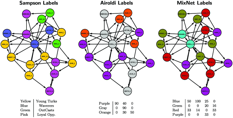
Monk	Sampson label	MMSB label	MixNet label
Ambrose	LO	Gray	Green
Boniface	YT	Violet	Green
Mark	YT	Violet	Purple
Winfrid	YT	Violet	Green
Elias	O	Orange	Red
Basil	O	Orange	Green
Simplicius	O	Orange	Green
Berthold	LO	Gray	Purple
John	YT	Violet	Purple
Victor	W	Gray	Red
Bonaventure	LO	Gray	Blue
Amand	W	Orange	Green
Louis	LO	Gray	Red
Albert	YT	Violet	Red
Ramuald	W	Gray	Blue
Peter	LO	Gray	Red
Gregory	YT	Violet	Red
Hugh	YT	Violet	Purple

Joint distribution

Since MixNet is defined by its conditional distribution, we first check that the joint distribution also belongs to the exponential family. Using notation

$$\cases{N_{q}(\mathbf{Z})=\displaystyle\sum_{i}Z_{iq},\vspace*{2pt}\cr H_{ql}(\mathbf{X},\mathbf{Z})=\displaystyle\sum_{ij}Z_{iq}Z_{jl}h(X_{ij}),\vspace*{2pt}\cr G_{ql}(\mathbf{Z})=\displaystyle\sum_{ij}Z_{iq}Z_{jl}=N_{q}(\mathbf{Z})N_{l}(\mathbf{Z}),\vspace*{2pt}\cr\alpha_{q}=\exp(\omega_{q})/\displaystyle\sum_{l}\exp(\omega_{l})}$$

and

$$\cases{T(\mathbf{X},\mathbf{Z})=(\{N_{q}(\mathbf{Z})\},\{H_{ql}(\mathbf{X},\mathbf{Z})\},\{G_{ql}(\mathbf{Z})\}),\vspace*{2pt}\cr\bolds{\beta}=(\{\omega_{q}\},\{\eta_{ql}\},\{-a(\eta_{ql})\}),\vspace*{2pt}\cr A(\bolds{\beta})=n\log\displaystyle\sum_{l}\exp\omega_{l},\vspace*{2pt}\cr B(\mathbf{X})=\displaystyle\sum_{ij}b(X_{ij}),}$$

we have the factorization $\log\Pr\{\mathbf{X},\mathbf{Z};\bolds{\beta}\}=\bolds{\beta}^{t}T(\mathbf{X},\mathbf{Z})-A(\bolds{\beta})+B(\mathbf{X}),$ which proves the claim. The sufficient statistics $T(\mathbf{X},\mathbf{Z})$ of the complete-data model are the number of nodes in the classes $N_{q}(\mathbf{Z})$, the characteristics of the between-group links ($H_{ql}$ through function $h$ that can stand for the number of between group links or for the intensity of the connections in the case of edges with Poisson or Gaussian distributions), and the product of frequencies between classes $G_{ql}$. In the following we aim at estimating $\bolds{\beta}$.

3.2 Sufficient statistics and online recursion

Online algorithms are incremental algorithms which recursively update parameters, using current parameters and new observations. We introduce the following notation. Let us denote by $\mathbf{X}^{[n]}=\{X_{ij}\}_{i,j=1}^{n}$ the adjacency matrix of the data, when $n$ nodes are present, and by $\mathbf{Z}^{[n]}$ the associated labels. A convenient notation in this context is $\mathbf{X}_{i,\bullet}=\{X_{ij},j\in\mathcal{V}\}$, which denotes all the edges related to node $i$. Note that the addition of one node leads to the addition of $n+1$ potential connections.

The use of online methods is based on the additivity of the sufficient statistics regarding the addition of a new node. We can show that

$$\cases{N_{q}\bigl{(}\mathbf{Z}^{[n+1]}\bigr{)}=N_{q}\bigl{(}\mathbf{Z}^{[n]}\bigr{)}+Z_{n+1,q},\vspace*{2pt}\cr H_{ql}\bigl{(}\mathbf{X}^{[n+1]},\mathbf{Z}^{[n+1]}\bigr{)}=H_{ql}\bigl{(}\mathbf{X}^{[n]},\mathbf{Z}^{[n]}\bigr{)}+\xi_{ql}^{[n+1]},\vspace*{2pt}\cr G_{ql}\bigl{(}\mathbf{Z}^{[n+1]}\bigr{)}=G_{ql}\bigl{(}\mathbf{Z}^{[n]}\bigr{)}+\zeta_{ql}^{[n+1]},}$$

with

$$\xi_{ql}^{[n+1]} = Z_{n+1,q}\sum_{j=1}^{n}Z_{jl}h(X_{n+1,j})+Z_{n+1,l}\sum_{i=1}^{n}Z_{iq}h(X_{i,n+1}),$$

$$\zeta_{ql}^{[n+1]} = Z_{n+1,q}N_{l}^{[n]}+Z_{n+1,l}N_{q}^{[n]}+Z_{n+1,q}I\{q=l\}.$$

Then if we define $T(\mathbf{X}_{n+1,\bullet},\mathbf{Z}^{[n+1]})=(Z_{n+1,q},\{\xi_{ql}^{[n+1]}\},\{\zeta_{ql}^{[n+1]}\})$, we get

$$T\bigl{(}\mathbf{X}^{[n+1]},\mathbf{Z}^{[n+1]}\bigr{)}=T\bigl{(}\mathbf{X}^{[n]},\mathbf{Z}^{[n]}\bigr{)}+T\bigl{(}\mathbf{X}_{n+1,\bullet},\mathbf{Z}^{[n+1]}\bigr{)}.$$ (1)

Those equations will be used for parameter updates in the online algorithms.

3.3 Likelihoods and online inference

Existing estimation strategies are based on maximum likelihood, and algorithms related to EM are used for optimization purposes. The aim is to maximize the conditional expectation of the complete-data log-likelihood

$$\mathcal{Q}(\bolds{\beta}|\bolds{\beta}^{\prime})=\sum_{\mathbf{Z}}\Pr\{\mathbf{Z}|\mathbf{X};\bolds{\beta}^{\prime}\}\log\Pr\{\mathbf{X},\mathbf{Z};\bolds{\beta}\},$$

and the main difficulty is that $\Pr\{\mathbf{Z}|\mathbf{X};\bolds{\beta}^{\prime}\}$ cannot be factorized and needs to be approximated [Daudin, Picard and Robin (2008)]. A first strategy to simplify the problem is to consider a classification EM-based strategy [Celeux and Govaert (1992)]. In this setting label variables are considered as nonrandom and are replaced by their prediction (0$/$1). This is a generalization of the $k$-means algorithm for which the problem of computing $\Pr\{\mathbf{Z}|\mathbf{X}\}$ is left apart. This strategy has been the subject of a previous work [Zanghi, Ambroise and Miele (2008)]. It is known to give biased estimates, but is very efficient from a computational time point of view.

To this strategy, we propose two different alternatives based on the Stochastic Approximation EM approach [Delyon, Lavielle and Moulines (1999)] which approximates $\Pr\{\mathbf{Z}|\mathbf{X}\}$ using Monte Carlo simulations, and on the so-called variational approach, which consists of approximating $\Pr\{\mathbf{Z}|\mathbf{X}\}$ by a more tractable distribution on the hidden variables. In their online versions, these algorithms optimize $\mathcal{Q}(\bolds{\beta}|\bolds{\beta}^{\prime})$ sequentially, while nodes are added. To this extent, we introduce notation

$$\mathcal{Q}_{n+1}\bigl{(}\bolds{\beta}|\bolds{\beta}^{[n]}\bigr{)}=\sum_{\mathbf{Z}^{[n+1]}}\Pr\bigl{\{}\mathbf{Z}^{[n+1]}|\mathbf{X}^{[n+1]};\bolds{\beta}^{[n]}\bigr{\}}\log\Pr\bigl{\{}\mathbf{X}^{[n+1]},\mathbf{Z}^{[n+1]};\bolds{\beta}\bigr{\}},$$

with $[n+1]$ being either the number of nodes or the increment of the algorithm, which are identical in the online context.

4 Stochastic approximation EM for network mixture

4.1 A short presentation of SAEM

An original way of estimating the parameters of the MixNet model is to approximate the expectation of the complete data log-likelihood using Monte Carlo simulations corresponding to the Stochastic Approximation EM algorithm [Delyon, Lavielle and Moulines (1999)]. In situations where maximizing $\mathcal{Q}(\bolds{\beta}|\bolds{\beta}^{\prime})$ is not in a simple closed form, the SAEM algorithm maximizes an approximation $\widehat{\mathcal{Q}}(\bolds{\beta}|\bolds{\beta}^{\prime})$ computed using standard stochastic approximation theory such that

$$\widehat{\mathcal{Q}}(\bolds{\beta}|\bolds{\beta}^{\prime})^{[k]}=\widehat{\mathcal{Q}}(\bolds{\beta}|\bolds{\beta}^{\prime})^{[k-1]}+\rho_{k}\bigl{(}\widetilde{\mathcal{Q}}(\bolds{\beta}|\bolds{\beta}^{\prime})-\widehat{\mathcal{Q}}(\bolds{\beta}|\bolds{\beta}^{\prime})^{[k-1]}\bigr{)},$$ (2)

where $k$ is an iteration index, $\{\rho_{k}\}_{k\geq 1}$ a sequence of positive step size and where $\widetilde{Q}(\bolds{\beta}|\bolds{\beta}^{\prime})$ is obtained by Monte Carlo integration. This is a simulation of the expectation of the complete log-likelihood using the posterior $\Pr\{\mathbf{Z}|\mathbf{X}\}$. Each iteration $k$ of the algorithm is broken down into three steps:

Simulation

of the missing data. This can be achieved using Gibbs Sampling of the posterior $\Pr\{\mathbf{Z}|\mathbf{X}\}$. The result at iteration number $k$ is $m(k)$ realizations of the latent class data $\mathbf{Z}$: $(\mathbf{Z}({1}),\ldots,\mathbf{Z}({m(k)}))$.

Stochastic approximation

of $\mathcal{Q}(\bolds{\beta}|\bolds{\beta}^{\prime})$ using equation (2), with

$$\widetilde{\mathcal{Q}}(\bolds{\beta}|\bolds{\beta}^{\prime})=\frac{1}{m(k)}\sum_{s=1}^{m(k)}\log\Pr(\mathbf{X},\mathbf{Z}(s);\bolds{\beta}).$$ (3)

Maximization

of $\widehat{\mathcal{Q}}(\bolds{\beta}|\bolds{\beta}^{\prime})^{[k]}$ according to $\bolds{\beta}$.

As regards the online version of the algorithm, the number of iterations $k$ usually coincides with $n+1$, the number of nodes of the network. Although it is possible to go further in the iterative process to improve the estimates, it is rarely necessary since the results obtained with $n+1$ iterations are usually reliable. This can be explained by the fact that the MixNet model is robust to sampling. The information in the network is indeed highly redundant and a reliable estimation of the network parameters can be obtained with a small sample (a few dozen) of the nodes using a classical batch algorithm. When $n$ is large, using an online algorithm with all the nodes is similar to performing many iterations of a batch algorithm on a small sample.

4.2 Simulation of $\Pr\{\mathbf{Z}|\mathbf{X}\}$ in the online context

We use Gibbs sampling which is applicable when the joint distribution is not known explicitly, but the conditional distribution of each variable is known. Here we generate a sequence of $\mathbf{Z}$ approaching $\Pr\{\mathbf{Z}|\mathbf{X}\}$ using $\Pr\{Z_{iq}=1|\mathbf{X},\mathbf{Z}_{\backslash i}\}$, where $\mathbf{Z}_{\backslash i}$ stands for the class of all nodes except node $i$. The sequence of samples is a Markov chain, and the stationary distribution of this Markov chain corresponds precisely to the joint distribution we wish to obtain. In the online context, we consider only one simulation to simulate the class of the last incoming node using

$$\Pr\bigl{\{}Z_{n+1,q}=1|\mathbf{X}^{[n+1]},\mathbf{Z}^{[n]}\bigr{\}}$$

$$\qquad=\frac{\Pr\{Z_{n+1,q}=1,\mathbf{Z}^{[n]},\mathbf{X}^{[n+1]}\}}{\sum_{\ell=1}^{Q}\Pr\{Z_{n+1,\ell}=1,\mathbf{Z}^{[n]},\mathbf{X}^{[n+1]}\}}.$$

$$\qquad=\frac{\exp\{\bolds{\beta}^{t}T(\mathbf{X}_{n+1,\bullet},\mathbf{Z}^{[n]},Z_{n+1,q})\}}{\sum_{\ell=1}^{Q}\exp\{\bolds{\beta}^{t}T(\mathbf{X}_{n+1,\bullet},\mathbf{Z}^{[n]},Z_{n+1,\ell})\}}$$

$$\qquad\propto\exp\Biggl{(}\omega_{q}+\sum_{\ell=1}^{Q}\eta_{q\ell}\sum_{j=1}^{n}Z_{j\ell}h(X_{n+1,j})+\sum_{\ell=1}^{Q}N_{\ell}\bigl{(}\mathbf{Z}^{[n]}\bigr{)}a(\eta_{q\ell})\Biggr{)}.$$

4.3 Computing $\widehat{\mathcal{Q}}(\mathbf{\beta}|\mathbf{\beta}^{\prime})$ in the online context

As regards the online version of the SAEM algorithm, the difference between the old and the new complete-data log-likelihood may be expressed as

$$\log\Pr\bigl{(}\mathbf{X}^{[n+1]},\mathbf{Z}^{[n+1]},\bolds{\beta}\bigr{)}-\log\Pr\bigl{(}\mathbf{X}^{[n]},\mathbf{Z}^{[n]},\bolds{\beta}\bigr{)}$$

$$\qquad=\log\alpha_{q}+\sum_{l,i<n+1}Z_{il}\log\Pr\{X_{n+1,i}|Z_{n+1,q}Z_{il}\},$$

where the added simulated vertex label is equal to $q$ ($Z_{n+1,q}=1$).

Recall that in the online framework, the label of the new node has been sampled from the Gibbs sampler described in Section 4.2. Consequently, only one possible label is considered in this equation. Then a natural way to adapt equation (2) to the online context is to approximate

$$\widetilde{\mathcal{Q}}_{n+1}\bigl{(}\bolds{\beta}|\bolds{\beta}^{[n]}\bigr{)}-\widehat{\mathcal{Q}}_{n}\bigl{(}\bolds{\beta}|\bolds{\beta}^{[n]}\bigr{)}$$

by

$$\log\Pr\bigl{(}\mathbf{X}^{[n+1]},\mathbf{Z}^{[n+1]},\bolds{\beta}\bigr{)}-\log\Pr\bigl{(}\mathbf{X}^{[n]},\mathbf{Z}^{[n]},\bolds{\beta}\bigr{)}.$$

Indeed, this quantity corresponds to the difference between the log-likelihood of the original network and log-likelihood of the new network including the additional node. Notice that the larger the network, the larger its associated complete expected log-likelikelihood. Thus, $\log\Pr(\mathbf{X}^{[n+1]},\mathbf{Z}^{[n+1]},\bolds{\beta})$ becomes smaller and smaller compared to ${Q}(\bolds{\beta}|\bolds{\beta}^{\prime})$ as $n$ increases. The decreasing step $\rho_{n}$ is thus set to one in this online context. We propose the following update equation for stochastic online EM computation of the MixNet conditional expectation:

$$\widehat{\mathcal{Q}}_{n+1}\bigl{(}\bolds{\beta}|\bolds{\beta}^{[n]}\bigr{)}=\widehat{\mathcal{Q}}_{n}\bigl{(}\bolds{\beta}|\bolds{\beta}^{[n]}\bigr{)}+\log\alpha_{q}+\sum_{l,i<n+1}Z_{il}\log\Pr\{X_{n+1,i}|Z_{n+1,q}Z_{il}\},$$

where $\mathbf{Z}_{n+1}$ is drawn from the Gibbs sampler.

4.4 Maximizing $\widehat{\mathcal{Q}}(\mathbf{\beta}|\mathbf{\beta}^{\prime})$, and parameters update

The principle of online algorithms is to modify the current parameter estimation using the information added by a new available $[n+1]$ node and its corresponding connections $\mathbf{X}_{n+1,\bullet}$ to the already existing network. Maximizing $\widehat{\mathcal{Q}}_{n+1}(\bolds{\beta}|\bolds{\beta}^{[n]})$ according to $\bolds{\beta}$ is straightforward and produces the maximum likelihood estimates for iteration $[n+1]$. Here we have proposed a simple version of the algorithm by setting the number of simulations to one ($m(k)=1$). In this context, the difference between $\widehat{\mathcal{Q}}_{n}(\bolds{\beta}|\bolds{\beta}^{[n]})$ and $\widehat{\mathcal{Q}}_{n+1}(\bolds{\beta}|\bolds{\beta}^{[n]})$ implies only the terms of the complete log-likelihood which are a function of node $n+1$. Using notation $\psi_{ql}=\frac{\partial a(\eta_{ql})}{\partial\eta_{ql}},$ we get

$$\cases{\alpha_{q}^{[n+1]}=N_{q}\bigl{(}\mathbf{Z}^{[n+1]}\bigr{)}/(n+1),\vspace*{2pt}\cr\psi_{ql}^{[n+1]}=H_{ql}\bigl{(}\mathbf{X}^{[n+1]},\mathbf{Z}^{[n+1]}\bigr{)}/G_{ql}\bigl{(}\mathbf{Z}^{[n+1]}\bigr{)},}$$

where $(\xi_{ql},\zeta_{ql})$ were defined in the previous section. Notice that updating the function $\psi_{ql}$ of the parameter of interest is often more convenient in an online context than directly considering this parameter of interest. An example of parameter update is given for the Bernoulli and Poisson cases in the Appendix.

Once all the nodes in the network have been visited (or are known), the parameters can be further improved and the complete log-likelihood better approximated by continuing with the SAEM algorithm described above.

5 Application of online algorithm to variational methods

Variational methods constitute an alternative to SAEM. Their principle is to approximate the untractable distribution $\Pr\{\mathbf{Z}|\mathbf{X};\bolds{\beta}\}$ by a newly introduced distribution on $\mathbf{Z}$ denoted by $\mathcal{R}$. Then this new distribution is used to optimize $\mathcal{J}(\mathbf{X},\mathcal{R}(\mathbf{Z});\bolds{\beta})$, an approximation (lower bound) of the incomplete-data log-likelihood $\log\Pr\{\mathbf{X};\bolds{\beta}\}$, defined such that

$$\mathcal{J}(\mathbf{X},\mathcal{R}(\mathbf{Z});\bolds{\beta})=\log\Pr\{\mathbf{X};\bolds{\beta}\}-\mathit{KL}(\mathcal{R}(\mathbf{Z}),\Pr\{\mathbf{Z}|\mathbf{X};\bolds{\beta}\}),$$

with $\mathit{KL}(\bullet|\bullet)$ being the Kullback–Leibler divergence between probability distributions [Jordan et al. (1999)]. Then one must choose the form of $\mathcal{R}$, and the product of Multinomial distributions is natural in the case of MixNet, with $\log\mathcal{R}(\mathbf{Z})=\sum_{i}\sum_{q}Z_{iq}\log\tau_{iq},$ and the constraint $\sum_{q}\tau_{iq}=1$. In this case, the form of $\mathcal{J}(\mathbf{X},\mathcal{R}(\mathbf{Z});\bolds{\beta})$ is

$$\mathcal{J}(\mathbf{X},\mathcal{R}(\mathbf{Z});\bolds{\beta}) = \sum_{\mathbf{Z}}\mathcal{R}(\mathbf{Z};\bolds{\tau})\log\Pr\{\mathbf{X},\mathbf{Z};\bolds{\beta}\}-\sum_{\mathbf{Z}}\mathcal{R}(\mathbf{Z};\bolds{\tau})\log\mathcal{R}(\mathbf{Z};\bolds{\tau})$$

$$= \mathcal{Q}(\bolds{\tau},\bolds{\beta})+\mathcal{H}(\mathcal{R}(\mathbf{Z};\bolds{\tau})),$$

with $\mathcal{Q}(\bolds{\tau},\bolds{\beta})$ an approximation of the conditional expectation of the complete-data log-likelihood, and $\mathcal{H}(\mathcal{R}(\mathbf{Z};\bolds{\tau}))$ the entropy of the approximate posterior distribution of $\mathbf{Z}$.

The implementation of variational methods in online algorithms relies on the additivity property of $\mathcal{J}(\mathbf{X},\mathcal{R}(\mathbf{Z});\bolds{\beta})$ when nodes are added. This property is straightforward: $\mathcal{Q}(\bolds{\tau},\bolds{\beta})$ is additive thanks to equation (1) [because $\mathcal{R}(\mathbf{Z})$ is factorized], and $\mathcal{H}(\mathcal{R}(\mathbf{Z};\bolds{\tau}))$ is also additive, since the hidden variables are supposed independent under $\mathcal{R}$ and the entropy of independent variables is additive. The variational algorithm is very similar to an EM algorithm, with the E-step being replaced by a variational step which aims at updating variational parameters. Then a standard M-step follows. In the following, we give the details of these two steps in the case of a variational online algorithm.

5.1 Online variational step

When a new node is added, it is necessary to compute its associated variational parameters $\{\tau_{n+1,q}\}_{q}$. If we consider all the other $\tau_{iq}$ for $i<n+1$ as known, the $\{\tau_{n+1,q}\}_{q}$ are obtained by differentiating the criterion

$$\mathcal{J}\bigl{(}\mathbf{X}^{[n+1]},\mathcal{R}\bigl{(}\mathbf{Z}^{[n+1]}\bigr{)};\bolds{\beta}\bigr{)}+\sum_{i=1}^{n+1}\Lambda_{i}\Biggl{(}\sum_{q=1}^{Q}\tau_{iq}-1\Biggr{)},$$

where the $\Lambda_{i}$ are the Lagrangian parameters. Since function $\mathcal{J}$ is additive according to the nodes, the calculation of its derivative according to $\tau_{n+1,q}$ gives

$$\omega_{q}^{[n]}+\sum_{l=1}^{Q}\sum_{j=1}^{n}\tau_{jl}^{[n]}\bigl{(}\eta_{ql}^{[n]}h(X_{n+1,j})+a\bigl{(}\eta_{ql}^{[n]}\bigr{)}\bigr{)}-\log\tau_{n+1,q}+1+\Lambda_{n+1}=0.$$

This leads to

$$\tau_{n+1,q}\propto\alpha_{q}^{[n]}\exp\Biggl{\{}\sum_{l=1}^{Q}\sum_{j=1}^{n}\tau_{jl}^{[n]}\bigl{(}\eta_{ql}^{[n]}h(X_{n+1,j})+a\bigl{(}\eta_{ql}^{[n]}\bigr{)}\bigr{)}\Biggr{\}}$$

$$\eqntext{\forall q\in\{1,\ldots,Q\}.}$$ (5)

5.2 Maximization/update step

To maximize the approximated expectation of the complete log-likelihood according to $\bolds{\beta}$, we solve

$$\frac{\partial\mathcal{Q}_{n+1}(\bolds{\tau},\bolds{\beta})}{\partial\bolds{\beta}}=\mathbb{E}_{\mathcal{R}^{[n]}}\biggl{(}\frac{\partial\log\Pr\{\mathbf{X}^{[n+1]},\mathbf{Z}^{[n+1]};\bolds{\beta}\}}{\partial\bolds{\beta}}\biggr{)}=0.$$ (6)

Differentiating equation (6) with respect to parameters $\{\omega_{q}\}$ gives the following update equation:

$$\alpha_{q}^{[n+1]}=\frac{1}{n+1}\Biggl{(}\sum_{i=1}^{n}\tau_{iq}^{[n]}+\tau_{n+1,q}\Biggr{)}.$$

The other update equation is obtained by considering parameters $\{\eta_{ql}\}$, and using notation $\psi_{ql}$, which gives

$${\psi}_{ql}^{n+1}=\frac{\mathbb{E}_{\mathcal{R}^{[n]}}(H_{ql}(\mathbf{X}^{[n+1]},\mathbf{Z}^{[n+1]}))}{\mathbb{E}_{\mathcal{R}^{[n]}}(G_{ql}(\mathbf{Z}^{[n+1]}))}.$$

Thanks to equation (1), which gives the relationships between sufficient statistics at two successive iterations, parameters can be computed recursively using the update of the expectation of the sufficient statistics, such that

$$\mathbb{E}_{\mathcal{R}^{[n]}}\bigl{(}N_{q}\bigl{(}\mathbf{Z}^{[n+1]}\bigr{)}\bigr{)} = \mathbb{E}_{\mathcal{R}^{[n]}}\bigl{(}N_{q}\bigl{(}\mathbf{Z}^{[n]}\bigr{)}\bigr{)}+\mathbb{E}_{\mathcal{R}^{[n]}}(Z_{n+1,q}),$$

$$\mathbb{E}_{\mathcal{R}^{[n]}}\bigl{(}H_{ql}\bigl{(}\mathbf{X}^{[n+1]},\mathbf{Z}^{[n+1]}\bigr{)}\bigr{)} = \mathbb{E}_{\mathcal{R}^{[n]}}\bigl{(}H_{ql}\bigl{(}\mathbf{X}^{[n]},\mathbf{Z}^{[n]}\bigr{)}\bigr{)}+\mathbb{E}_{\mathcal{R}^{[n]}}\bigl{(}\xi_{ql}^{[n+1]}\bigr{)},$$

$$\mathbb{E}_{\mathcal{R}^{[n]}}\bigl{(}G_{ql}\bigl{(}\mathbf{Z}^{[n+1]}\bigr{)}\bigr{)} = \mathbb{E}_{\mathcal{R}^{[n]}}\bigl{(}G_{ql}\bigl{(}\mathbf{Z}^{[n]}\bigr{)}\bigr{)}+\mathbb{E}_{\mathcal{R}^{[n]}}\bigl{(}\zeta_{ql}^{[n+1]}\bigr{)}.$$

An example of parameters update is given in the Appendix for both the Bernoulli and the Poisson distributions. Note the similarity of the formula compared with the SAEM strategy. Hidden variables $\mathbf{Z}$ are either simulated or replaced by their approximated conditional expectation (variational parameters).

6 Experiments

Motivations

Experiments are carried out to assess the trade-off established by online algorithms in terms of quality of estimation and speed of execution. We propose a two-online-step simulation study. We first report simulation experiments using synthetic data generated according to the assumed random graph model. In this first experiment we use a simple affiliation model to check precisely the quality of the estimations given by the online algorithms. Results are compared to the batch variational EM proposed by Daudin, Picard and Robin (2008) to assess the effect of the online framework on the estimation quality and on the speed of execution. In a second step, we use a real data set from the web as a starting point to simulate growing networks with complex structure, and to assess the performance of online methods on this type of network. An ANSI C$++$ implementation of the algorithms is available at http://stat.genopole.cnrs.fr/software/mixnet/, as well as an R package named MixeR (http://cran.r-project.org/web/packages/mixer/), along with public data sets. This software is currently used by the Constellations online application (http://constellations.labs.exalead.com/), which instantaneously extracts, visually explores and takes advantages of the MixNet algorithm to reveal the connectivity information induced by hyperlinks between the first hits of a given search request.

6.1 Comparison of algorithms

Simulations set-up

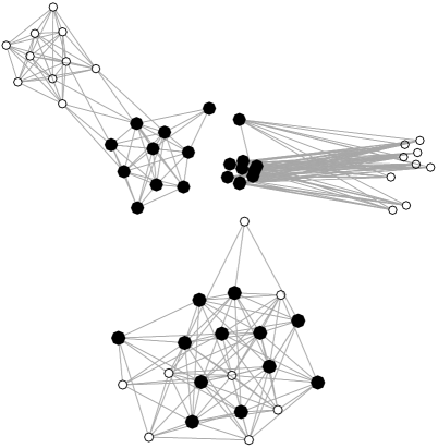
We simulate affiliation models with $\lambda$ and $\varepsilon$ being the within and between group probability of connection respectively. Five models are considered (Table 2). We set $\lambda=1-\varepsilon$ to reduce the number of free parameters, with parameter $\lambda$ controlling the complexity of the model. Differences between models lie in their modular structure which varies from no structure (almost the Erdős–Rényi model) to strong modular structure (low inter-module connectivity and strong intra-module connectivity, or strong inter-module connectivity and low intra-module connectivity). Figure 2 illustrates three kinds of connectivity which allows to represent graphically model 1, 4 and 5. For each affiliation model we generate graphs with $Q\in\{2,5,20\}$ groups mixed in the same proportions $1/Q$. The number of nodes $n$ varies in $\{100,250,500,750,1000,2000\}$ to explore different sizes of graphs. We generate a total of 45 graph models, each being simulated 30 times.

Figure 2: Top left: low inter-module connectivity and strong intra-module connectivity (model 1). Top right: strong inter-module connectivity and low intra-module connectivity (model 5). Bottom center: Erdős–Rényi model (model 4).

Table 2: Parameters of the five affiliation models considered in the experimental setting

Model	$\bolds{\varepsilon}$	$\bolds{\lambda}$
1	0.30	0.70
2	0.35	0.65
3	0.40	0.60
4	0.50	0.50
5	0.90	0.10

Criteria of comparison

The comparison between algorithms is done using the bias $\mathbb{E}(\varepsilon-\widehat{\varepsilon})/\varepsilon$ and the mean square error $\mathbb{V}(\widehat{\varepsilon})$ to reflect estimators variability. We also use the adjusted Rand Index [Hubert and Arabie (1985)] to evaluate the agreement between the estimated and the actual partitions. Computing this index is based on a ratio between the number of node pairs belonging to the same and to different classes when considering the actual partition and the estimated partition. It lies between 0 and 1, two identical partitions having an adjusted Rand Index equal to 1.

Algorithms set-up

In a first step we compete algorithms that are based on maximum likelihood estimation (MLE). The online SAEM and online variational method we propose are compared with the variational method proposed in Daudin, Picard and Robin (2008) (batch MixNet in the sequel). We also add an online classification version (online CEM) in the comparison since this strategy has been shown to reduce the computational cost as well [Zanghi, Ambroise and Miele (2008)]. To avoid initialization issues, each algorithm is started with the same strategy: multiple initialization points are proposed and the best result is selected based on its likelihood. The number of clusters is chosen using the Integrated Classification Likelihood criterion, as proposed in Daudin, Picard and Robin (2008). The algorithms are stopped when the parameters are stable between two consecutive iterations. In a second step, we compare the MLE-based algorithms with other competitors like spectral clustering [Ng, Jordan and Weiss (2002)] and a $k$-means like algorithm [Newman (2006)].

Estimators bias and MSE (Table 3)

A first result is that every algorithm provides estimators with negligible bias (lower than $1\%$) and variance for highly structured models (models 1, 2, 5, Table 3). The online framework shows its limitations when the structure of the network is less pronounced (model 3), as every online method shows a significant bias and low precision, whereas the batch MixNet behaves well. This limitation was expected, as the gain in computational burden has an impact on the complexity of structures that can be identified. Finally, among online versions of the algorithm, the online variational method provides the best results on average in terms of bias and precision.

Table 3: Bias (in percent) and Root Mean Square Errors ($\times\!10^{3}$) for the parameters estimators in the five affiliation models. The $Q$ modules are mixed in the same proportion. Each model considers $n=500$ nodes and $Q=5$ groups

	Online-SAEM		Online-variational		Online-CEM		Batch-MixNet
Model	$\mathbf{B}_{\bolds{\%}}\!\bolds{(\widehat{\varepsilon})}$	$\mathbf{B}_{\bolds{\%}}\!\bolds{(\widehat{\lambda})}$	$\mathbf{B}_{\bolds{\%}}\!\bolds{(\widehat{\varepsilon})}$	$\mathbf{B}_{\bolds{\%}}\!\bolds{(\widehat{\lambda})}$	$\mathbf{B}_{\bolds{\%}}\!\bolds{(\widehat{\varepsilon})}$	$\mathbf{B}_{\bolds{\%}}\!\bolds{(\widehat{\lambda})}$	$\mathbf{B}_{\bolds{\%}}\!\bolds{(\widehat{\varepsilon})}$	$\mathbf{B}_{\bolds{\%}}\!\bolds{(\widehat{\lambda})}$
1	$-0.14$	$0.04$	$-0.13$	$0.04$	$-0.13$	$0.04$	$-0.13$	$0.04$
2	$0.23$	$-1.01$	$0.04$	$-0.11$	$-0.03$	$0.01$	$-0.03$	$0.00$
3	$9.47$	$-26.38$	$8.83$	$-24.32$	$6.44$	$-22.46$	$-0.01$	$-0.11$
4	$1.11$	$-4.29$	$0.16$	$-0.35$	$3.00$	$-4.32$	$0.05$	$-0.01$
5	$-0.01$	$-0.02$	$-0.01$	$-0.02$	$-0.01$	$-0.02$	$-0.01$	$-0.02$
	RMSE($\widehat{\varepsilon})$	RMSE($\widehat{\lambda})$	RMSE($\widehat{\varepsilon})$	RMSE($\widehat{\lambda})$	RMSE($\widehat{\varepsilon})$	RMSE($\widehat{\lambda})$	RMSE($\widehat{\varepsilon})$	RMSE($\widehat{\lambda})$
1	$1.45$	$2.25$	$1.42$	$2.25$	$1.45$	$2.25$	$1.45$	$2.25$
2	$1.89$	$4.04$	$1.65$	$2.90$	$1.63$	$2.90$	$1.63$	$2.90$
3	$5.19$	$14.75$	$6.95$	$22.32$	$13.89$	$25.96$	$2.14$	$6.74$
4	$3.75$	$10.42$	$1.33$	$1.67$	$8.21$	$15.71$	$1.25$	$1.62$
5	$0.92$	$1.73$	$0.92$	$1.73$	$0.93$	$1.73$	$0.92$	$1.73$

Table 4: Means and standard deviations of the Rand Index for all models with $q$ and $n$ fixed

	Online-SAEM		Online-variational		Online-CEM		Batch-MixNet
Model	$\bolds{\overline{\mathit{rand}}}$	$\bolds{\sigma_{\mathit{rand}}}$	$\bolds{\overline{\mathit{rand}}}$	$\bolds{\sigma_{\mathit{rand}}}$	$\bolds{\overline{\mathit{rand}}}$	$\bolds{\sigma_{\mathit{rand}}}$	$\bolds{\overline{\mathit{rand}}}$	$\bolds{\sigma_{\mathit{rand}}}$
1	0.98	0.02	0.98	0.02	0.98	0.02	0.99	0.02
2	0.96	0.07	0.97	0.07	0.97	0.07	0.98	0.01
3	0.13	0.13	0.10	0.15	0.25	0.16	0.85	0.14
4	0.00	0.00	0.00	0.00	0.00	0.00	0.00	0.00
5	100	0.00	100	0.01	100	0.01	100	0.01

Quality of partitions (Table 4)

We also focus on the Rand Index for each algorithm. Indeed, even if poor estimation of $\lambda$ reveals a small Rand Index (Table 4), good estimates do not always lead to correctly estimated partitions. An illustration is given with model 3 for which algorithms produce good estimates with poor Rand Index, due to the nonmodular structure of the network. As expected, the performance increases with the number of nodes (Table 5).

Table 5: Means and standard deviations of the Rand Index with speed of the algorithms. $q=5$, model 2

	Online-SAEM		Online-variational		Online-CEM		Batch-MixNet
$\bolds{n}$	$\bolds{\overline{\mathit{rand}}}$	$\bolds{\sigma_{\mathit{rand}}}$	$\bolds{\overline{\mathit{rand}}}$	$\bolds{\sigma_{\mathit{rand}}}$	$\bolds{\overline{\mathit{rand}}}$	$\bolds{\sigma_{\mathit{rand}}}$	$\bolds{\overline{\mathit{rand}}}$	$\bolds{\sigma_{\mathit{rand}}}$
100	$0.15$	0.04	$0.15$	0.07	$0.15$	0.05	$0.19$	$0.09$
250	$0.50$	0.09	$0.55$	0.11	$0.51$	0.01	$0.95$	$0.07$
500	$0.62$	0.09	$0.62$	0.11	$0.65$	0.14	$1$	$0.00$
750	$0.84$	0.03	$0.85$	0.03	$0.84$	0.04	$1$	$0.00$
1000	$0.94$	0.01	$0.95$	0.01	$0.92$	9.37	$1$	$0.00$
2000	$0.98$	0.00	$0.98$	0.01	$0.98$	0.01	$1$	$0.00$
	$\overline{\mathit{time}}$	$\sigma_{\mathit{time}}$	$\overline{\mathit{time}}$	$\sigma_{\mathit{time}}$	$\overline{\mathit{time}}$	$\sigma_{\mathit{time}}$	$\overline{\mathit{time}}$	$\sigma_{\mathit{time}}$
100	$0.09$	0.00	$0.09$	0.00	$0.09$	0.00	$0.10$	$0.00$
250	$1.31$	0.01	$1.32$	0.01	$1.31$	0.00	$3.18$	$0.01$
500	$1.41$	0.01	$1.46$	0.01	$1.41$	0.01	$49.46$	$0.13$
750	$3.45$	0.02	$3.57$	0.02	$3.44$	0.02	$251.32$	$0.75$
1000	$9.46$	0.41	$9.61$	0.43	$9.37$	0.40	$805.92$	$0.49$
2000	$157.31$	1.28	$158.21$	1.41	$157.12$	2.08	$13051.10$	$73.75$

Computational efficiency (Table 5)

Since the aim of online methods is to provide computationally efficient algorithms, the performance mentioned above should be put in perspective with the speed of execution of each algorithm. Indeed, Table 5 shows the strong gain of speed provided by online methods compared with the batch algorithm. The speed of execution is divided by 100 on networks with 2000 nodes, for instance. Table 5 also shows that there is no significant difference in the speed of execution among online methods. Since the online variational method provides the best results in terms of estimation precision, with no significant difference with other methods on partition quality or speed, this will be the algorithm chosen for the following.

Comparison with other algorithms (Table 6)

The above results show that a strong case may be made for the online variational algorithm when choosing between alternative clustering methods. Consequently, we shall now compare it with two suitable “rivals” for large networks: a basic spectral clustering algorithm [Ng, Jordan and Weiss (2002)], and one of the popular community detection algorithms [Newman (2006)]. The spectral clustering algorithm searches for a partition in the space spanned by the eigenvectors of the normalized Laplacian, whereas the community detection algorithm looks for modules which are defined by high intra-connectivity and low inter-connectivity.

For our five models with arbitrary fixed parameters $n=1000$, $Q=3$, we ran these algorithms and computed the Rand Index for each of them. From Table 6 we see that our online variational algorithm always produces the best clustering of nodes.

Table 6: Means and standard deviation of the Rand Index for the five models computed over 30 different runs for graph clustering competitors and variational algorithms

	Community detection		Spectral clustering		Online-variational
Model	$\bolds{\overline{\mathit{rand}}}$	$\bolds{\sigma_{\mathit{rand}}}$	$\bolds{\overline{\mathit{rand}}}$	$\bolds{\sigma_{\mathit{rand}}}$	$\bolds{\overline{\mathit{rand}}}$	$\bolds{\sigma_{\mathit{rand}}}$
1	1.00	0.00	0.97	0.14	1.00	0.00
2	0.99	0.01	0.98	0.00	1.00	0.00
3	0.97	0.02	0.97	0.00	1.00	0.00
4	0.00	0.00	0.00	0.00	0.00	0.00
5	0.00	0.00	0.92	0.19	1.00	0.00

We generated networks using the MixNet data generating process. Thus, these results correspond to what may be expected on networks that display a blockmodel structure: the online variational algorithm always yields the best node classification. Apart from model 4, it will also be remarked that the spectral algorithm is fairly efficient with a slight bias, and so the spectral clustering algorithm is consistently more accurate than the community algorithm, the latter failing completely when applied to model 5. Although the community algorithm appears less well adapted to these experiments, we shall see in the next section that this algorithm is particularly suitable when partitioning data sets whose nodes are densely interconnected.

6.2 Realistic networks growing over time

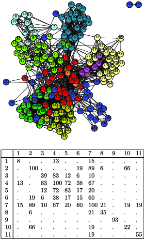
In this section we use a real network as a template to simulate a realistic complex structure. For this purpose, we use a French Political Blogosphere network data set that consists of a sample of 196 political blogs from a single day snapshot. This network was automatically extracted October 14, 2006 and manually classified by the “Observatoire Presidentielle” project. This project is the result of a collaboration between RTGI SAS and Exalead and aims at analyzing the French presidential campaign on the web. In this data set, nodes represent hostnames (a hostname contains a set of pages) and edges represent hyperlinks between different hostnames. If several links exist between two different hostnames, we collapse them into a single one. Note that intra-domain links can be considered if hostnames are not identical. Finally, in this experimentation we consider that edges are not oriented, which is not realistic but which does not affect the interpretation of the groups. Six known communities compose this network: Gauche (French Democrat), Divers Centre (Moderate party), Droite (French Republican), Ecologiste (Green), Liberal (supporters of economic-liberalism) and, finally, Analysts. The data is provided within the MixeR package. This network presents an interesting organization due to the existence of several political parties and commentators. This complex connectivity pattern is enhanced by MixNet parameters given in Figure 3.

Figure 3: MixNet results display on the French political Blogosphere represented with the organic layout of Cytoscape (Shannon et al., 2003). The table corresponds to the probabilities ($\times\!100$) of connection between the 11 selected clusters [using a penalized likelihood criterion described in Daudin, Picard and Robin (2008)]. Dots in the table correspond to connections lower than $1\%$.

As the algorithm is motivated by large data sets, we use the parameters given by MixNet to generate networks that grow over time. We use this French Blog to generate a realistic network structure as a start point. We simulate 200 nodes networks from this model, then we iterate by simulating the growth over time of these networks according to the same model and we use the online algorithm to update parameters sequentially. The result is striking: even on very large networks with $\sim$13,000 nodes and $\sim$13,000,000 edges, the online algorithm allows us to estimate mixture parameters with negligible classification error in $\sim$6 minutes (Table 7). This is the only algorithmic framework that allows to perform model based clustering on networks of that size.

7 Application to the 2008 US Presidential WebSphere

Since its creation and enhanced by its recent social aspect (Web 2.0), the World Wide Web is the space where individuals use Internet technologies to talk, discuss and debate. Such space can be seen as a directed graph where the pages and hyperlinks are respectively represented by nodes and edges. From this graph, many studies, like Broder et al. (2000), have been published and introduced the key properties of the Web structure. However, this section rather focuses on local studies by considering that the Web is formed by territories and communities with their own conversation leaders and participants [Ghitalla et al. (2003)]. Here, we define a territory as a group of websites concerned by the same topic and a community as a group of websites in the same territory which may share the same opinion or the same link connectivity. One usually assumes that the existence of a hyperlink between two pages implies that they are content-related [Kleinberg (1999); Davison (2000)]. By exploring the link page exchanges, one can actually draw the borders of web territories/communities.

Comparison with a community detection algorithm

A first step consists in comparing the results of MixNet with the community detection algorithm proposed by Newman (2006). If the political classification is used as a reference, the community algorithm produces better agreement with a $\mathit{randIndex}=0.59$, compared with a $\mathit{randIndex}=0.25$ for MixNet (see Table 8). However, it appears that this comparison favors Newman, whereas the methods have different objective. Indeed, the community algorithm aims at finding modules which are defined by high intra-connectivity and low inter-connectivity. Given that websites tend to link to one another in line with political affinities, the link topology corresponding to the manual classification naturally favors the community module definition. The objective function can also help to explain the community algorithm’s suitability for this data set, since the quality of a partition in terms of Newman’s modules can be expressed in terms of the modularity, which is maximized. The value of this modularity is a scalar between $-$1 and 1 and measures the density of links inside communities as compared to links between communities [Newman (2006)]. When applying both algorithms on our political network with $Q=3$, the online variational algorithm yields a $\mathit{modularity}=0.20$, whereas the community algorithm yields a $\mathit{modularity}=0.30$, which is close to the manual partition modularity of 0.28. As MixNet classes do not necessarily take the form of modules, one might expect our approach to yield a modularity index that is not “optimal.” Nevertheless, the two class definitions are complementary, and both are needed in order to give a global overview of a network: the community partition to detect dense node connectivity, and the MixNet partition to analyze nodes with similar connectivity profiles. However, as mentioned by Adamic and Glance (2005), the division between liberal and conservative blogs is “unmistakable,” this is why it may be more interesting to uncover the structure of the two communities rather than detecting them.

Table 7: Quality of the clustering procedure in terms of Rand Index when the network grows over time. Each configuration has been simulated 100 times

$\bolds{\#}$ nodes (previous${}\bolds{+}{}$new)	00.Ave. $\bolds{\#}$ edges	Ave. rand	Ave. cpu time (s)
200	00000.003131.72	$0.94$	$0.9$
200 $+$ 200	00000050,316.32	$0.998$	$0.4$
400 $+$ 400	00000012,486.24	$0.999$	$1.4$
800 $+$ 800	0000201,009.5	$1$	$5.7$
1600 $+$ 1600	0000803,179.6	$1$	$22.8$
3200 $+$ 3200	03,202,196	$1$	$91.9$
6400 $+$ 6400	12,804,008	$1$	$371.1$

Table 8: Contingency table comparing the political partition and MixNet partition

	Conservative	Independent	Liberal
Cluster 1	734	135	238
Cluster 2	290	026	008
Cluster 3	002	007	430

Interpreting MixNet results

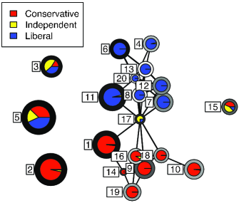
MixNet first confirms what was already mentioned by Adamic and Glance (2005): the political websphere is partioned according to political orientations. In addition, MixNet highlights the role of main US online portals as the core of this websphere (Figure 4, C17). Political communities do not directly cite their opponents but communicate through nytimes.com, washingtonpost.com, cnn.com or msn.com, for instance (in C17). This central structure has two main significations: it confirms the political cyberbalkanization trend that was already observed in 2004, and it emphasizes the role of mass media websites as political referees. Plus, the connectivity pattern estimated by the model shows a particular affinity between the mass-media cluster with the liberal thought, as connections are stronger toward the liberal part of the weblogs (Table 9).

Figure 4: Network summary of US political websites. Each vertex represents a cluster. Each pie chart gives the proportions of liberal, conservative and independent tagged websites in the cluster. The outer ring color of the vertices is proportional to the intensity of the intra-connectivity: the darker, the weaker. Edges are represented when the inter-connectivity is among the 20% of the largest among all connectivity values.

Table 9: Estimated $\pi$ (in percentage) and number of nodes in each cluster for the US political websphere. $\bar{d}$ represents the estimated mean degree of each group. Clusters with probabilities of connection lower than $1\%$ are not represented (clusters 3, 5, 15)

	Conservative								Liberal
ID	17	1	2	10	9	14	16	18	19	11	4	6	7	8	12	13	20
17	$\cdot$	$54$	$\cdot$	$\cdot$	$64$	$\cdot$	$52$	$66$	$\cdot$	$62$	$\cdot$	$\cdot$	$67$	$67$	$62$	$43$	$100$
1	$54$	$\cdot$	$\cdot$	$\cdot$	$\cdot$	$54$	$\cdot$	$\cdot$	$\cdot$	$\cdot$	$\cdot$	$\cdot$	$\cdot$	$\cdot$	$\cdot$	$\cdot$	$\cdot$
2	$\cdot$	$\cdot$	$\cdot$	$\cdot$	$\cdot$	$\cdot$	$\cdot$	$\cdot$	$\cdot$	$\cdot$	$\cdot$	$\cdot$	$\cdot$	$\cdot$	$\cdot$	$\cdot$	$\cdot$
10	$\cdot$	$\cdot$	$\cdot$	$58$	$\cdot$	$\cdot$	$\cdot$	$47$	$\cdot$	$\cdot$	$\cdot$	$\cdot$	$\cdot$	$\cdot$	$\cdot$	$\cdot$	$\cdot$
9	$64$	$\cdot$	$\cdot$	$\cdot$	$\cdot$	$56$	$61$	$\cdot$	$40$	$\cdot$	$\cdot$	$\cdot$	$\cdot$	$\cdot$	$\cdot$	$\cdot$	$\cdot$
14	$\cdot$	$54$	$\cdot$	$\cdot$	$56$	$\cdot$	$55$	$72$	$40$	$\cdot$	$\cdot$	$\cdot$	$\cdot$	$\cdot$	$\cdot$	$\cdot$	$\cdot$
16	$52$	$\cdot$	$\cdot$	$\cdot$	$61$	$55$	$73$	$60$	$56$	$\cdot$	$\cdot$	$\cdot$	$\cdot$	$\cdot$	$\cdot$	$\cdot$	$\cdot$
18	$66$	$\cdot$	$\cdot$	$47$	$\cdot$	$72$	$60$	$58$	$\cdot$	$\cdot$	$\cdot$	$\cdot$	$\cdot$	$\cdot$	$\cdot$	$\cdot$	$\cdot$
19	$\cdot$	$\cdot$	$\cdot$	$\cdot$	$40$	$40$	$56$	$\cdot$	$57$	$\cdot$	$\cdot$	$\cdot$	$\cdot$	$\cdot$	$\cdot$	$\cdot$	$\cdot$
11	$62$	$\cdot$	$\cdot$	$\cdot$	$\cdot$	$\cdot$	$\cdot$	$\cdot$	$\cdot$	$\cdot$	$\cdot$	$\cdot$	$\cdot$	$47$	$\cdot$	$\cdot$	$40$
4	$\cdot$	$\cdot$	$\cdot$	$\cdot$	$\cdot$	$\cdot$	$\cdot$	$\cdot$	$\cdot$	$\cdot$	$65$	$\cdot$	$\cdot$	$\cdot$	$\cdot$	$42$	$40$
6	$\cdot$	$\cdot$	$\cdot$	$\cdot$	$\cdot$	$\cdot$	$\cdot$	$\cdot$	$\cdot$	$\cdot$	$\cdot$	$\cdot$	$\cdot$	$\cdot$	$\cdot$	$88$	$99$
7	$67$	$\cdot$	$\cdot$	$\cdot$	$\cdot$	$\cdot$	$\cdot$	$\cdot$	$\cdot$	$\cdot$	$\cdot$	$\cdot$	$47$	$76$	$49$	$\cdot$	$76$
8	$67$	$\cdot$	$\cdot$	$\cdot$	$\cdot$	$\cdot$	$\cdot$	$\cdot$	$\cdot$	$47$	$\cdot$	$\cdot$	$76$	$90$	$74$	$81$	$98$
12	$62$	$\cdot$	$\cdot$	$\cdot$	$\cdot$	$\cdot$	$\cdot$	$\cdot$	$\cdot$	$\cdot$	$\cdot$	$\cdot$	$49$	$74$	$45$	$92$	$98$
13	$43$	$\cdot$	$\cdot$	$\cdot$	$\cdot$	$\cdot$	$\cdot$	$\cdot$	$\cdot$	$\cdot$	$42$	$88$	$\cdot$	$81$	$92$	$95$	$99$
20	$100$	$\cdot$	$\cdot$	$\cdot$	$\cdot$	$\cdot$	$\cdot$	$\cdot$	$\cdot$	$40$	$42$	$99$	$76$	$98$	$98$	$99$	$100$
$N_{q}$	$4$	$214$	$407$	$66$	$56$	$1$	$24$	$19$	$36$	$26$	$58$	$207$	$51$	$20$	$37$	$23$	$3$
$\bar{d}$	$649$	$86$	$28$	$149$	$69$	$455$	$335$	$167$	$172$	$192$	$64$	$66$	$66$	$310$	$154$	$170$	$324$

Then the question is to determine what are the structural characteristics of the liberal and conservative territories (note that independent sites do not seem to be structured on their own). MixNet reveals a hierarchical organization of political sub-spheres with weblogs having a determinant role in the structuration of the liberal community, reachm.com, mahablog.com, juancole.com (C20), which are well known to be at the core of the liberal debate on the web. This results in a set of clusters (C7, C8, C12, C13 and C20) that show very strong intra $and$ inter group connectivities which nearly forms a clique (Table 9). The balkanization is also observed within territories, as radical positions, like in the feministe.us website (C6), are only spread through core websites ($\hat{\pi}_{20,6}=99\%$, for instance). A last level of hierarchy is made by liberal blogs that show intermediate connections within the same liberal territory.

Interestingly, this subdivision is also present in the conservative part of the network, with very famous websites like foxnews.com (C14) being at the center of the debate. Indeed, clusters C3, C14, C16, C18 and C19 constitute the core of the conservative websphere, and clusters C1 and C2 are very lightly connected with other conservative blogs. The difference lies in the intensity of connection, which is lower for the conservatives.

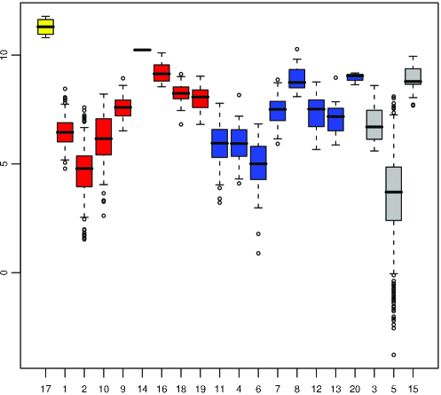
Compared with available methods that can analyze networks of such size (like community detection), MixNet shows structures of the political websphere that are more complex than the expected liberal/conservative split. The model highlights the structural similarities that exist between spheres of political opponents. Both communities are characterized by a small set of sites which use the internet in a very professional and efficient way, with a lot of cross-linking. This results in a core structure to which other sites are linked, these other sites being less efficient in the citations to other websites. This could be explained either by a tendency to ignore other elements in the debate or by a use of the internet which is less efficient. Interestingly, this structure is very similar between conservatives and liberals, with the liberal core being more tight. For the liberal blogs, this observation can result from a better understanding of their Web Ecosystem. This interpretation is reinforced by the different betweenness centralities of MixNet classes. Betweenness is based on the number of shortest geodesic paths that pass through a vertex. Figure 5 shows that MixNet betweenness is higher for MixNet core classes on average in both political structures, whereas the betweenness patterns of the liberals and conservatives look very similar.

Figure 5: Boxplot of MixNet classes betweenness (in log).

8 Conclusion

In this paper we propose an online version of estimation algorithms for random graphs which are based on a mixture of distributions. These strategies allow the estimation of model parameters within a reasonable computation time for data sets which can be made up of thousands of nodes. These methods constitute a trade-off between the potential amount of data to process and the quality of the estimations: even if online methods are not as precise as batch methods for estimation, they may represent a solution when the size of the network is too large for any existing estimation strategy. Furthermore, our simulation study shows that the quality of the remaining partition is good when using online methods. In the network of 2008 US political websites, we could uncover the structure that makes the political websphere. This structure is very different from classical modules or “communities,” which highlights the need for efficient computational strategies to perform model-based clustering on large graphs. The online framework is very flexible, and could be applied to other models such as the block model and the mixed membership model, as the online framework can be adapted to Bayesian algorithms [Opper (1999)].

Appendix

.1 Examples of distributions for the exponential family

We provide some examples of common distributions that can be used in the context of networks. For example, when the only available information is the presence or the absence of an edge, then $X_{ij}$ is assumed to follow a Bernoulli distribution:

$$X_{ij}|Z_{iq}Z_{jl}=1\sim\mathcal{B}(\pi_{ql})\cases{\eta_{ql}=\log\displaystyle\frac{\pi_{ql}}{1-\pi_{ql}},\vspace*{2pt}\cr h(X_{ij})=X_{ij},\vspace*{2pt}\cr a(\eta_{ql})=\log(1-\pi_{ql}),\vspace*{2pt}\cr b(X_{ij})=0.}$$

If additional information is available to describe the connections between vertices, it may be integrated into the model. For example, the Poisson distribution might describe the intensity of the traffic between nodes. A typical example in web access log mining is the number of users going from a page $i$ to a page $j$. Another example is provided by co-authorship networks, for which valuation may describe the number of articles commonly published by the authors of the network. In those cases, we have

$$X_{ij}|Z_{iq}Z_{jl}=1\sim\mathcal{P}(\lambda_{ql})\cases{\eta_{ql}=\log\lambda_{ql},\vspace*{2pt}\cr h(X_{ij})=X_{ij},\vspace*{2pt}\cr a(\eta_{ql})=-\lambda_{ql},\vspace*{2pt}\cr b(X_{ij})=X_{ij}!}$$

.2 Parameters update in the Bernoulli and Poisson cases for the online SAEM

The estimator becomes

$$\pi_{ql}^{[n+1]}=\gamma_{ql}^{[n+1]}\pi_{ql}^{[n]}+\bigl{(}1-\gamma_{ql}^{[n+1]}\bigr{)}\frac{\xi_{ql}^{[n+1]}}{\zeta_{ql}^{[n+1]}},$$

where

$$\gamma_{ql}^{[n+1]} = \frac{N_{q}(\mathbf{Z}^{[n]})N_{l}(\mathbf{Z}^{[n]})}{N_{q}(\mathbf{Z}^{[n]})N_{l}(\mathbf{Z}^{[n]})+Z_{n+1,q}N_{l}(\mathbf{Z}^{[n]})+Z_{n+1,l}N_{q}(\mathbf{Z}^{[n]})},$$

$$\xi_{ql}^{[n+1]} = Z_{n+1,q}\sum_{j=1}^{n}Z_{jl}^{[n]}X_{n+1,j}+Z_{n+1,l}\sum_{i=1}^{n}Z_{iq}^{[n]}X_{i,n+1},$$

$$\zeta_{ql}^{[n+1]} = Z_{n+1,q}N_{l}\bigl{(}\mathbf{Z}^{[n]}\bigr{)}+Z_{n+1,l}N_{q}\bigl{(}\mathbf{Z}^{[n]}\bigr{)}+Z_{n+1,q}\mathbb{I}\{q=l\}.$$

.3 Parameters update in the Bernoulli and the Poisson cases for the online variational algorithm

We get the following update equation:

$$\pi_{ql}^{[n+1]}=\gamma_{ql}^{[n+1]}\pi_{ql}^{[n]}+\bigl{(}1-\gamma_{ql}^{[n+1]}\bigr{)}\frac{\mathbb{E}_{\mathcal{R}^{[n]}}(\xi_{ql}^{[n+1]})}{\mathbb{E}_{\mathcal{R}^{[n]}}(\zeta_{ql}^{[n+1]})},$$

where

$$\gamma_{ql}^{[n+1]} = {\mathbb{E}_{\mathcal{R}^{[n]}}\bigl{(}N_{q}\bigl{(}\mathbf{Z}^{[n]}\bigr{)}\bigr{)}\mathbb{E}_{\mathcal{R}^{[n]}}\bigl{(}N_{l}\bigl{(}\mathbf{Z}^{[n]}\bigr{)}\bigr{)}}$$

$${}/\mathbb{E}_{\mathcal{R}^{[n]}}\bigl{(}N_{q}\bigl{(}\mathbf{Z}^{[n]}\bigr{)}\bigr{)}\mathbb{E}_{\mathcal{R}^{[n]}}\bigl{(}N_{l}\bigl{(}\mathbf{Z}^{[n]}\bigr{)}\bigr{)}+\tau_{n+1,q}\mathbb{E}_{\mathcal{R}^{[n]}}\bigl{(}N_{l}\bigl{(}\mathbf{Z}^{[n]}\bigr{)}\bigr{)}$$

$${}+\tau_{n+1,l}\mathbb{E}_{\mathcal{R}^{[n]}}\bigl{(}N_{q}\bigl{(}\mathbf{Z}^{[n]}\bigr{)}\bigr{)},$$

$$\mathbb{E}_{\mathcal{R}^{[n]}}\bigl{(}\xi_{ql}^{[n+1]}\bigr{)} = \tau_{n+1,q}\sum_{j=1}^{n}\tau_{jl}^{[n]}X_{n+1,j}+\tau_{n+1,l}\sum_{i=1}^{n}\tau_{iq}^{[n]}X_{i,n+1},$$

$$\mathbb{E}_{\mathcal{R}^{[n]}}\bigl{(}\zeta_{ql}^{[n+1]}\bigr{)} = \tau_{n+1,q}\mathbb{E}_{\mathcal{R}^{[n]}}\bigl{(}N_{l}\bigl{(}\mathbf{Z}^{[n]}\bigr{)}\bigr{)}+\tau_{n+1,l}\mathbb{E}_{\mathcal{R}^{[n]}}\bigl{(}N_{q}\bigl{(}\mathbf{Z}^{[n]}\bigr{)}\bigr{)}+\tau_{n+1,q}\mathbb{I}\{q=l\}$$

with

$$\mathbb{E}_{\mathcal{R}^{[n]}}\bigl{(}N_{q}\bigl{(}\mathbf{Z}^{[n]}\bigr{)}\bigr{)}=\sum_{i=1}^{n}\tau_{iq}^{[n]}.$$

References

- Adamic and Glance (2005) {barticle}[author] \bauthor\bsnmAdamic, \bfnmL.A.\binitsL. and \bauthor\bsnmGlance, \bfnmN.\binitsN. (\byear2005). \btitleThe political blogosphere and the 2004 US election: Divided they blog. In \bjournalProceedings of the 3rd International Workshop on Link Discovery \bpages36–43. ACM Press, New York. \endbibitem
- Airoldi et al. (2007) {binproceedings}[author] \bauthor\bsnmAiroldi, \bfnmE.M.\binitsE., \bauthor\bsnmBlei, \bfnmD.M.\binitsD., \bauthor\bsnmFienberg, \bfnmS.E.\binitsS. and \bauthor\bsnmXing, \bfnmE.P.\binitsE. (\byear2007). \btitleCombining Stochastic block models and mixed membership for statistical network analysis. In \bbooktitleStatistical Network Analysis: Models, Issues, and New Directions. \bseriesLecture Notes in Computer Science \bvolume4503 \bpages57–74. \bpublisherSpringer, Berlin. \endbibitem
- Airoldi et al. (2008) {barticle}[author] \bauthor\bsnmAiroldi, \bfnmE.M.\binitsE., \bauthor\bsnmBlei, \bfnmD.M.\binitsD., \bauthor\bsnmFienberg, \bfnmS.E.\binitsS. and \bauthor\bsnmXing, \bfnmE.P.\binitsE. (\byear2008). \btitleMixed-membership stochastic blockmodels. \bjournalJ. Mach. Learn. Res. \bvolume9 \bpages1981–2014. \endbibitem
- Airoldi et al. (2005) {binproceedings}[author] \bauthor\bsnmAiroldi, \bfnmE.M.\binitsE., \bauthor\bsnmBlei, \bfnmD.M.\binitsD., \bauthor\bsnmXing, \bfnmE.P.\binitsE. and \bauthor\bsnmFienberg, \bfnmS.E.\binitsS. (\byear2005). \btitleA latent mixed-membership model for relational data. In \bbooktitle3rd International Workshop on Link Discovery, Issues, Approaches and Applications; 11th International ACM SIGKDD Conference \bpages82–89. \bpublisherACM Press, New York. \endbibitem
- Bickel and Chen (2009) {barticle}[author] \bauthor\bsnmBickel, \bfnmP.J.\binitsP. and \bauthor\bsnmChen, \bfnmA.\binitsA. (\byear2009). \btitleA nonparametric view of network models and Newman–Girvan and other modularities. \bjournalProc. Natl. Acad. Sci. USA \bvolume106 \bpages21068–21073. \endbibitem
- Broder et al. (2000) {barticle}[author] \bauthor\bsnmBroder, \bfnmA.\binitsA., \bauthor\bsnmKumar, \bfnmR.\binitsR., \bauthor\bsnmMaghoul, \bfnmF.\binitsF., \bauthor\bsnmRaghavan, \bfnmP.\binitsP., \bauthor\bsnmRajagopalan, \bfnmS.\binitsS., \bauthor\bsnmStata, \bfnmR.\binitsR., \bauthor\bsnmTomkins, \bfnmA.\binitsA. and \bauthor\bsnmWiener, \bfnmJ.\binitsJ. (\byear2000). \btitleGraph structure in the web. \bjournalComputer Networks \bvolume33 \bpages309–320. \endbibitem
- Celeux and Govaert (1992) {barticle}[author] \bauthor\bsnmCeleux, \bfnmG.\binitsG. and \bauthor\bsnmGovaert, \bfnmG.\binitsG. (\byear1992). \btitleA Classification EM algorithm for clustering and two stochastic versions. \bjournalComput. Statist. Data Anal. \bvolume14 \bpages315–332. \MR1192205 \endbibitem
- Daudin, Picard and Robin (2008) {barticle}[author] \bauthor\bsnmDaudin, \bfnmJ.J.\binitsJ., \bauthor\bsnmPicard, \bfnmF.\binitsF. and \bauthor\bsnmRobin, \bfnmS.\binitsS. (\byear2008). \btitleA mixture model for random graph. \bjournalStatist. Comput. \bvolume18 \bpages1–36. \MR2390817 \endbibitem
- Davison (2000) {binproceedings}[author] \bauthor\bsnmDavison, \bfnmBrian D.\binitsB. D. (\byear2000). \btitleTopical locality in the Web. In \bbooktitleSIGIR’00: Proceedings of the 23rd Annual International ACM SIGIR Conference on Research and Development in Information Retrieval \bpages272–279. \bpublisherACM Press, \baddressNew York. \endbibitem
- Delyon, Lavielle and Moulines (1999) {barticle}[author] \bauthor\bsnmDelyon, \bfnmB.\binitsB., \bauthor\bsnmLavielle, \bfnmM.\binitsM. and \bauthor\bsnmMoulines, \bfnmE.\binitsE. (\byear1999). \btitleConvergence of a stochastic approximation version of the EM algorithm. \bjournalAnn. Statist. \bvolume27 \bpages94–128. \MR1701103 \endbibitem
- Dempster, Laird and Rubin (1977) {barticle}[author] \bauthor\bsnmDempster, \bfnmA. P.\binitsA. P., \bauthor\bsnmLaird, \bfnmN. M.\binitsN. M. and \bauthor\bsnmRubin, \bfnmD. B.\binitsD. B. (\byear1977). \btitleMaximum-likelihood from incomplete data via the EM algorithm. \bjournalJ. Roy. Statist. Soc. B \bvolume39 \bpages1–39. \MR0501537 \endbibitem
- Drugeon (2005) {barticle}[author] \bauthor\bsnmDrugeon, \bfnmT.\binitsT. (\byear2005). \btitleA technical approach for the French web legal deposit. In \bjournal5th International Web Archiving Workshop (IWAW05), Vienna. \endbibitem
- Fouetillou (2007) {barticle}[author] \bauthor\bsnmFouetillou, \bfnmG.\binitsG. (\byear2007). \btitleLe Web et le traité constitutionnel européen, écologie d’une localité thématique. \bjournalRéseaux \bvolume144 \bpages279–304. \endbibitem
- Ghitalla et al. (2003) {bbook}[author] \bauthor\bsnmGhitalla, \bfnmF.\binitsF., \bauthor\bsnmBoullier, \bfnmD.\binitsD., \bauthor\bsnmGkouskou, \bfnmP.\binitsP., \bauthor\bsnmLe Douarin, \bfnmL.\binitsL. and \bauthor\bsnmNeau, \bfnmA.\binitsA. (\byear2003). \btitleL’outre-lecture: manipuler, (s’) approprier, interpréter le Web. \bpublisherBibliothèque publique d’information Centre Pompidou. \endbibitem
- Handcock, Raftery and Tantrum (2007) {barticle}[author] \bauthor\bsnmHandcock, \bfnmMS.\binitsM., \bauthor\bsnmRaftery, \bfnmA.\binitsA. and \bauthor\bsnmTantrum, \bfnmJ.M.\binitsJ. (\byear2007). \btitleModel based clustering for social networks. \bjournalJ. Roy. Statist. Soc. Ser. A \bvolume170 301–354. \MR2364300 \endbibitem
- Hubert and Arabie (1985) {barticle}[author] \bauthor\bsnmHubert, \bfnmL.\binitsL. and \bauthor\bsnmArabie, \bfnmP.\binitsP. (\byear1985). \btitleComparing partitions. \bjournalJ. Classification \bvolume2 \bpages193–218. \endbibitem
- Jordan et al. (1999) {barticle}[author] \bauthor\bsnmJordan, \bfnmM.I.\binitsM., \bauthor\bsnmGhahramani, \bfnmZ.\binitsZ., \bauthor\bsnmJaakkola, \bfnmT.S.\binitsT. and \bauthor\bsnmSaul, \bfnmL.K.\binitsL. (\byear1999). \btitleAn introduction to variational methods for graphical models. \bjournalMach. Learn. \bvolume37 \bpages183–233. \endbibitem
- Kleinberg (1999) {barticle}[author] \bauthor\bsnmKleinberg, \bfnmJ.M.\binitsJ. (\byear1999). \btitleAuthoritative sources in a hyperlinked environment. \bjournalJ. ACM \bvolume46 \bpages604–632. \MR1747649 \endbibitem
- Latouche, Birmele and Ambroise (2008) {btechreport}[author] \bauthor\bsnmLatouche, \bfnmP.\binitsP., \bauthor\bsnmBirmele, \bfnmE.\binitsE. and \bauthor\bsnmAmbroise, \bfnmC.\binitsC. (\byear2008). \btitleBayesian methods for graph clustering. Statistics for Systems Biology, \btypeTechnical Report No. \bnumber17. \endbibitem
- Liu et al. (2006) {barticle}[author] \bauthor\bsnmLiu, \bfnmZ.\binitsZ., \bauthor\bsnmAlmhana, \bfnmJ.\binitsJ., \bauthor\bsnmChoulakian, \bfnmV.\binitsV. and \bauthor\bsnmMcGorman, \bfnmR.\binitsR. (\byear2006). \btitleOnline EM algorithm for mixture with application to internet traffic modeling. \bjournalComput. Statist. Data Anal. \bvolume50 \bpages1052–1071. \MR2210745 \endbibitem
- MacQueen (1967) {barticle}[author] \bauthor\bsnmMacQueen, \bfnmJ.\binitsJ. (\byear1967). \btitleSome methods for classification and analysis of multivariate observations. In \bjournalProc. Fifth Berkeley Sympos. Math. Statist. Probab. \bvolume1 \bpages281–296. Univ. California Press, Berkeley, CA. \MR0214227 \endbibitem
- Newman (2006) {barticle}[author] \bauthor\bsnmNewman, \bfnmMEJ\binitsM. (\byear2006). \btitleModularity and community structure in networks. \bjournalProc. Natl. Acad. Sci. USA \bvolume103 \bpages8577–8582. \endbibitem
- Newman and Leicht (2007) {barticle}[author] \bauthor\bsnmNewman, \bfnmME.\binitsM. and \bauthor\bsnmLeicht, \bfnmEA.\binitsE. (\byear2007). \btitleMixture models and exploratory analysis in networks. \bjournalProc. Natl. Acad. Sci. USA \bvolume104 \bpages9564–9569. \endbibitem
- Ng, Jordan and Weiss (2002) {binproceedings}[author] \bauthor\bsnmNg, \bfnmA.Y.\binitsA., \bauthor\bsnmJordan, \bfnmM.\binitsM. and \bauthor\bsnmWeiss, \bfnmY.\binitsY. (\byear2002). \btitleOn spectral clustering: Analysis and an algorithm. In \bbooktitleNeural Information Processing System 14 849–856. MIT Press, Cambridge, MA. \endbibitem
- Nowicki and Snijders (2001) {barticle}[author] \bauthor\bsnmNowicki, \bfnmKrzysztof\binitsK. and \bauthor\bsnmSnijders, \bfnmTom A. B.\binitsT. A. B. (\byear2001). \btitleEstimation and prediction for stochastic blockstructures. \bjournalJ. Amer. Statist. Assoc. \bvolume96 \bpages1077–1090. \MR1947255 \endbibitem
- Opper (1999) {binbook}[author] \bauthor\bsnmOpper, \bfnmManfred\binitsM. (\byear1999). A Bayesian approach to online learning. \btitleOn-Line Learning in Neural Networks 16 \bpages363–378. \bpublisherCambridge Univ. Press, Cambridge, MA. \endbibitem
- Picard et al. (2009) {barticle}[author] \bauthor\bsnmPicard, \bfnmF.\binitsF., \bauthor\bsnmMiele, \bfnmV.\binitsV., \bauthor\bsnmDaudin, \bfnmJJ.\binitsJ., \bauthor\bsnmCottret, \bfnmL.\binitsL. and \bauthor\bsnmRobin, \bfnmS.\binitsS. (\byear2009). \btitleDeciphering the connectivity structure of biological networks using MixNet. \bjournalBMC Bioinformatics \bvolume10 \bpages1–11. \endbibitem
- Salton, Wong and Yang (1975) {barticle}[author] \bauthor\bsnmSalton, \bfnmG.\binitsG., \bauthor\bsnmWong, \bfnmA.\binitsA. and \bauthor\bsnmYang, \bfnmCS\binitsC. (\byear1975). \btitleA vector space model for automatic indexing. \bjournalCommun. ACM \bvolume18 \bpages613–620. \endbibitem
- Sampson (1968) {bphdthesis}[author] \bauthor\bsnmSampson, \bfnmF. S.\binitsF. S. (\byear1968). \btitleA novitiate in a period of change: An experimental and case study of social relationship. \btypePh.D. thesis, \bschoolCornell Univ. \endbibitem
- Shannon et al. (2003) {barticle}[author] \bauthor\bsnmShannon, \bfnmP.\binitsP., \bauthor\bsnmMarkiel, \bfnmA.\binitsA., \bauthor\bsnmOzier, \bfnmO.\binitsO., \bauthor\bsnmBaliga, \bfnmNS.\binitsN., \bauthor\bsnmWang, \bfnmJT.\binitsJ., \bauthor\bsnmRamage, \bfnmD.\binitsD., \bauthor\bsnmAmin, \bfnmN.\binitsN., \bauthor\bsnmSchwikowski, \bfnmB.\binitsB. and \bauthor\bsnmIdeker, \bfnmT.\binitsT. (\byear2003). \btitleCytoscape: A software environment for integrated models of biomolecular interaction networks. \bjournalGenome Res. \bvolume13 \bpages2498–2504. \endbibitem
- Snijders and Nowicki (1997) {barticle}[author] \bauthor\bsnmSnijders, \bfnmT. A. B.\binitsT. A. B. and \bauthor\bsnmNowicki, \bfnmK.\binitsK. (\byear1997). \btitleEstimation and prediction for stochastic block-structures for graphs with latent block structure. \bjournalJ. Classification \bvolume14 \bpages75–100. \MR1449742 \endbibitem
- Titterington (1984) {barticle}[author] \bauthor\bsnmTitterington, \bfnmD. M.\binitsD. M. (\byear1984). \btitleRecursive parameter estimation using incomplete data. \bjournalJ. Roy. Statist. Soc. Ser. B \bvolume46 \bpages257–267. \MR0781884 \endbibitem
- Wang and Zhao (2006) {barticle}[author] \bauthor\bsnmWang, \bfnmS.\binitsS. and \bauthor\bsnmZhao, \bfnmY.\binitsY. (\byear2006). \btitleAlmost sure convergence of Titterington’s recursive estimator for finite mixture models. \bjournalStatist. Probab. Lett. \bvolume76 \bpages2001–2006. \MR2329245 \endbibitem
- Zanghi, Ambroise and Miele (2008) {barticle}[author] \bauthor\bsnmZanghi, \bfnmH.\binitsH., \bauthor\bsnmAmbroise, \bfnmC.\binitsC. and \bauthor\bsnmMiele, \bfnmV.\binitsV. (\byear2008). \btitleFast online graph clustering via Erdős–Rényi mixture. \bjournalPattern Recognition \bvolume41 \bpages3592–3599. \endbibitem