Suppression of oscillations by Lévy noise

Abstract

We find analytical solution of pair of stochastic equations with arbitrary forces and multiplicative Lévy noises in a steady-state nonequilibrium case. This solution shows that Lévy flights suppress always a quasi-periodical motion related to the limit cycle. We prove that such suppression is caused by that the Lévy variation $\Delta L\sim(\Delta t)^{1/\alpha}$ with the exponent $\alpha<2$ is always negligible in comparison with the Gaussian variation $\Delta W\sim(\Delta t)^{1/2}$ in the $\Delta t\to 0$ limit. Moreover, this difference is shown to remove the problem of the calculus choice because related addition to the physical force is of order $(\Delta t)^{2/\alpha}\ll\Delta t$.

1 Introduction

It is known crucial changing in behavior of the systems that display noise-induced [1, 2] and recurrence [3, 4] phase transitions, stochastic resonance [5, 6], noise induced pattern formation [7, 8], noise induced transport [9, 2] etc. is caused by interplay between noise and non-linearity (see Ref. [10], for review). Noises of different origin can play a constructive role in dynamical behavior such as hopping between multiple stable attractors [11, 12] and stabilization of the Lorenz attractor near the threshold of its formation [13, 14]. This type of behavior is inherent in finite systems where examples of substantial alteration under effect of intrinsic noises give epidemics [15]–[17], predator-prey population dynamics [18, 19], opinion dynamics [20], biochemical clocks [21, 22], genetic networks [23], cyclic trapping reactions [24] et cetera.

Above pointed out phase transitions present the simplest case, when joint effect of both noise and non-linearity arrives at non-trivial fixed point appearance only on the phase-plane of the system states. In this consideration, we are interested in studying much more complicated situation, when stochastic system may display oscillatory behavior related to the limit cycle appearing as a result of the Hopf bifurcation [25, 26]. It has long been conjectured [27] that in some situations the influence of noise would be sufficient to produce cyclic behavior [28]. Moreover, it has been shown that excitable [29], bistable [30] and close to bifurcations [31] systems display oscillation behavior, whose adjacency to ideally periodic signal depends resonantly on the noise intensity [32] (due to this reason, such oscillations were been called coherence resonance [29] or stochastic coherence [10]).

Characteristic peculiarity of above considerations is that all of them are restricted by studying the Gaussian noise effect, while such a noise is a special case of the Lévy stable process (the principle difference of these noises is known [33] to consist in the form of the probability distribution that exhibits the asymptotic power-law decay in the latter case and decays exponentially in the former one). Nowadays, anomalous diffusion processes associated with the Lévy stable noise are attracting much attention in a vast variety of fields not only of natural sciences (physics, biology, earth science, and so on), but of social sciences such as risk management, finance, etc.

In the context of physics, recent investigation has shown that joint effect of both non-linearity and Lévy noise may cause the occurrence of genuine phase transitions which relates to a fixed point on the phase-plane of the system states. In this connection, natural question arises: may be displayed a self-organized quasi-periodical behavior related to the limit cycle by a system driven by the Lévy stable noise? This work is devoted to the answer to above question within analytical study of two-dimensional stochastic system.

The paper is organized as follows. In Section 2, we consider pair of stochastic equations with arbitrary forces and multiplicative Lévy noises to obtain their analytical solution in a steady-state nonequilibrium case. This allows us to conclude in Section 3 that opposite to the Gaussian noises the Lévy flights suppress always a quasi-periodical motion related to the limit cycle. Since equation, governing behavior of stochastic system driven by multiplicative Lévy stable noise, are very complicated [35] and moreover their derivation is now in progress [36], we complete our consideration with Appendix A containing details of derivation of the Fokker-Planck equation. Moreover, to demonstrate that a closed consideration of the Lévy processes is achieved only within the Fourier representation we set forth a scheme related to the appropriate stochastic space in Appendix B.

2 Statistical picture of limit cycle

According to the theorem of central manifold [25], to achieve a closed description of a limit cycle it is enough to use only two degrees of freedom related to some stochastic variables $X_{i}$, $i=1,2$. In this way, stochastic evolution of the system under investigation is defined by the Langevin equations [37]

$${\rm d}X_{i}=f_{i}{\rm d}t+g_{i}{\rm d}L_{i},\quad i=1,2$$ (1)

with arbitrary forces $f_{i}=f_{i}(x_{1},x_{2})$ and noise amplitudes $g_{i}=g_{i}(x_{1},x_{2})$ being functions of both variables $x_{i}$, $i=1,2$; stochastic terms are related to the Lévy stable processes $L_{i}=L_{i}(t)$. Within the Îto calculus, these processes are determined by the elementary characteristic function

$$\left<{\rm e}^{{\rm i}k_{i}{\rm d}X_{i}}\right>:={\rm e}^{\mathcal{L}_{i}{\rm d}t}$$ (2)

with increments $\mathcal{L}_{i}=\mathcal{L}_{i}(k_{1},k_{2};x_{1},x_{2})$ whose expression [35]

$$\mathcal{L}_{i}={\rm i}k_{i}\left(f_{i}+\gamma_{i}g_{i}\right)-|m_{i}g_{i}k_{i}|^{\frac{\alpha}{2}}{\rm e}^{-{\rm i}\varphi_{i}(\frac{\alpha}{2})}\sum\limits_{j=1}^{2}\left|m_{j}g_{j}k_{j}\right|^{\frac{\alpha}{2}}{\rm e}^{-{\rm i}\varphi_{j}(\frac{\alpha}{2})}$$ (3)

follows from Eq.(A.25). Hereafter, we use asymmetry angles $\varphi_{i}$ and moduli $m_{i}$ defined by the equalities

$$\begin{split}\tan\left[\varphi_{i}(\alpha)\right]&=\beta_{i}{\rm sgn}(g_{i}k_{i})\tan(\pi\alpha/2),\\ m_{i}^{\alpha}&=\sqrt{1+\beta_{i}^{2}\tan^{2}(\pi\alpha/2)};\end{split}$$ (4)

everywhere, the Lévy index $\alpha\in(0,2)$ characterizes the asymptotic tail $x_{i}^{-(\alpha+1)}$ of the Lévy stable distribution at $1\neq\alpha<2$ (the case $\alpha=2$ relates to the Gaussian distribution), parameters $\beta_{i}\in[-1,+1]$ define the distribution asymmetry, location parameters $-\infty<\gamma_{i}<+\infty$ denote the mean values of stochastic variables $X_{i}$ at $\alpha>1$, and the angular brackets denote averaging over Lévy noises.

As is shown in Appendix A, the Fourier transformed probability distribution function

$$\widetilde{P}(k_{1},k_{2};t)\equiv\mathcal{F}\{P(x_{1},x_{2})\}(k_{1},k_{2};t):=\iint\limits_{-\infty}^{+\infty}{\rm d}x_{1}{\rm d}x_{2}~{}P(x_{1},x_{2};t){\rm e}^{{\rm i}\left(k_{1}x_{1}+k_{2}x_{2}\right)}$$ (5)

is governed by the Fokker-Planck equation

$$\frac{\partial\widetilde{P}}{\partial t}=\sum\limits_{i=1}^{2}\left[{\rm i}\left(f_{i}+\gamma_{i}g_{i}\right)k_{i}-|m_{i}g_{i}k_{i}|^{\frac{\alpha}{2}}{\rm e}^{-{\rm i}\varphi_{i}(\frac{\alpha}{2})}\sum\limits_{j=1}^{2}\left|m_{j}g_{j}k_{j}\right|^{\frac{\alpha}{2}}{\rm e}^{-{\rm i}\varphi_{j}(\frac{\alpha}{2})}\right]\widetilde{P}.$$ (6)

Characteristically, being Fourier transformed, r.h.s. of this equation depends on the wave vector components $k_{1}$ and $k_{2}$, while both forces $f_{i}=f_{i}(x_{1},x_{2})$ and multiplicative noise amplitudes $g_{i}=g_{i}(x_{1},x_{2})$ are dependent on the coordinate components $x_{1}$ and $x_{2}$.

According to the continuity equation (A.23), components of the steady-state probability flux are obeyed to the condition $\sum_{i}\partial J_{i}/\partial x_{i}=0$ which means the first component $J_{1}=J_{1}(x_{2})$ is a function of the only variable $x_{2}$, and vice-versa for the second component $J_{2}=J_{2}(x_{1})$. Then, within the Fourier representation, the system behaviour is defined by the equations

$$\begin{split}&\left\{\left(f_{1}+g_{1}\gamma_{1}\right)+{\rm i}|m_{1}g_{1}|^{\frac{\alpha}{2}}{\rm e}^{-{\rm i}\varphi_{1}\left(\frac{\alpha}{2}\right)}|k_{1}|^{\frac{\alpha}{2}-2}k_{1}\right.\\ &\left.\times\left[\left|m_{1}g_{1}k_{1}\right|^{\frac{\alpha}{2}}{\rm e}^{-{\rm i}\varphi_{1}\left(\frac{\alpha}{2}\right)}+\left|m_{2}g_{2}k_{2}\right|^{\frac{\alpha}{2}}{\rm e}^{-{\rm i}\varphi_{2}\left(\frac{\alpha}{2}\right)}\right]\right\}\widetilde{P}=2\pi J_{1}(k_{2})\delta(k_{1}),\end{split}$$ (7)

$$\begin{split}&\left\{\left(f_{2}+g_{2}\gamma_{2}\right)+{\rm i}|m_{2}g_{2}|^{\frac{\alpha}{2}}{\rm e}^{-{\rm i}\varphi_{2}\left(\frac{\alpha}{2}\right)}|k_{2}|^{\frac{\alpha}{2}-2}k_{2}\right.\\ &\left.\times\left[\left|m_{1}g_{1}k_{1}\right|^{\frac{\alpha}{2}}{\rm e}^{-{\rm i}\varphi_{1}\left(\frac{\alpha}{2}\right)}+\left|m_{2}g_{2}k_{2}\right|^{\frac{\alpha}{2}}{\rm e}^{-{\rm i}\varphi_{2}\left(\frac{\alpha}{2}\right)}\right]\right\}\widetilde{P}=2\pi J_{2}(k_{1})\delta(k_{2}).\end{split}$$ (8)

Since the pair of these equations determines a single distribution function $\widetilde{P}(k_{1},k_{2})$, the consistency condition

$$\begin{split}\left[\left(f_{1}+g_{1}\gamma_{1}\right)+{\rm i}{\rm e}^{-{\rm i}\varphi_{1}(\alpha)}|m_{1}g_{1}|^{\alpha}|k_{1}|^{\alpha-2}k_{1}\right]\delta(k_{2})J_{2}(k_{1})\\ =\left[\left(f_{2}+g_{2}\gamma_{2}\right)+{\rm i}{\rm e}^{-{\rm i}\varphi_{2}(\alpha)}|m_{2}g_{2}|^{\alpha}|k_{2}|^{\alpha-2}k_{2}\right]\delta(k_{1})J_{1}(k_{2})\end{split}$$ (9)

should be kept to restrict the choice of the probability flux components $J_{1}(k_{2})$ and $J_{2}(k_{1})$.

Multiplying Eq.(7) by the factor $|m_{2}g_{2}|^{\frac{\alpha}{2}}{\rm e}^{-{\rm i}\varphi_{2}\left(\frac{\alpha}{2}\right)}$ and Eq.(8) by $|m_{1}g_{1}|^{\frac{\alpha}{2}}{\rm e}^{-{\rm i}\varphi_{1}\left(\frac{\alpha}{2}\right)}$ and then subtracting results, one obtains

$$\begin{split}\left\{F+{\rm i}|m_{1}m_{2}g_{1}g_{2}|^{\frac{\alpha}{2}}{\rm e}^{-{\rm i}\left[\varphi_{1}\left(\frac{\alpha}{2}\right)+\varphi_{2}\left(\frac{\alpha}{2}\right)\right]}\right.\\ \left.\times\left[\left|m_{1}g_{1}k_{1}\right|^{\frac{\alpha}{2}}{\rm e}^{-{\rm i}\varphi_{1}\left(\frac{\alpha}{2}\right)}+\left|m_{2}g_{2}k_{2}\right|^{\frac{\alpha}{2}}{\rm e}^{-{\rm i}\varphi_{2}\left(\frac{\alpha}{2}\right)}\right]\left(|k_{1}|^{\frac{\alpha}{2}-2}k_{1}-|k_{2}|^{\frac{\alpha}{2}-2}k_{2}\right)\right\}\widetilde{P}\\ =2\pi\left[J_{1}(k_{2})\delta(k_{1})|m_{2}g_{2}|^{\frac{\alpha}{2}}{\rm e}^{-{\rm i}\varphi_{2}\left(\frac{\alpha}{2}\right)}-J_{2}(k_{1})\delta(k_{2})|m_{1}g_{1}|^{\frac{\alpha}{2}}{\rm e}^{-{\rm i}\varphi_{1}\left(\frac{\alpha}{2}\right)}\right]\end{split}$$ (10)

where one denotes

$$F\equiv\left(f_{1}+\gamma_{1}g_{1}\right)|m_{2}g_{2}|^{\frac{\alpha}{2}}{\rm e}^{-{\rm i}\varphi_{2}\left(\frac{\alpha}{2}\right)}-\left(f_{2}+\gamma_{2}g_{2}\right)|m_{1}g_{1}|^{\frac{\alpha}{2}}{\rm e}^{-{\rm i}\varphi_{1}\left(\frac{\alpha}{2}\right)}.$$ (11)

The equation (10) yields the explicit form of the probability distribution function

$$\begin{split}P\left(x_{1},x_{2}\right)&=\int\limits_{-\infty}^{+\infty}\frac{{\rm d}k_{2}}{2\pi}\frac{J_{1}(k_{2})|m_{2}g_{2}|^{\frac{\alpha}{2}}{\rm e}^{-{\rm i}\left[k_{2}x_{2}+\varphi_{2}\left(\frac{\alpha}{2}\right)\right]}}{F_{2}-{\rm i}|g_{1}|^{\frac{\alpha}{2}}|m_{2}g_{2}|^{\alpha}{\rm e}^{-{\rm i}\varphi_{2}\left(\alpha\right)}|k_{2}|^{\alpha-2}k_{2}}\\ &-\int\limits_{-\infty}^{+\infty}\frac{{\rm d}k_{1}}{2\pi}\frac{J_{2}(k_{1})|m_{1}g_{1}|^{\frac{\alpha}{2}}{\rm e}^{-{\rm i}\left[k_{1}x_{1}+\varphi_{1}\left(\frac{\alpha}{2}\right)\right]}}{F_{1}+{\rm i}|g_{2}|^{\frac{\alpha}{2}}|m_{1}g_{1}|^{\alpha}{\rm e}^{-{\rm i}\varphi_{1}\left(\alpha\right)}|k_{1}|^{\alpha-2}k_{1}}\end{split}$$ (12)

where effective forces $F_{1,2}$ are determined by Eq.(11) at $m_{2,1}=1$ and $\varphi_{2,1}=0$.

In the case of constant values of the probability flux within the state space $x_{1},x_{2}$, the Fourier transforms related are $J_{1}(k_{2})=2\pi J_{1}^{(0)}\delta(k_{2})$ and $J_{2}(k_{1})=2\pi J_{2}^{(0)}\delta(k_{1})$ with $J_{i}^{(0)}={\rm const}$. Then, the consistency condition (9) takes the form $\left(f_{1}+g_{1}\gamma_{1}\right)J_{2}^{(0)}=\left(f_{2}+g_{2}\gamma_{2}\right)J_{1}^{(0)}$, the effective force (11) is $F_{0}=\left(f_{1}+\gamma_{1}g_{1}\right)|g_{2}|^{\frac{\alpha}{2}}-\left(f_{2}+\gamma_{2}g_{2}\right)|g_{1}|^{\frac{\alpha}{2}}$, and the probability density (12) reads

$$P=\frac{J_{1}^{(0)}|g_{2}|^{\frac{\alpha}{2}}-J_{2}^{(0)}|g_{1}|^{\frac{\alpha}{2}}}{F_{0}}.$$ (13)

To create a limit cycle this distribution function should diverges on a closed curve, so that the effective force equals $F_{0}=0$. Together with the consistency condition, this equation gives

$$\frac{J_{1}^{(0)}}{J_{2}^{(0)}}=\frac{f_{1}+\gamma_{1}g_{1}}{f_{2}+\gamma_{2}g_{2}}=\left|\frac{g_{1}}{g_{2}}\right|^{\frac{\alpha}{2}}.$$ (14)

But these equalities mean that the numerator of the probability density (13) disappears also. As a result, we conclude the limit cycle creation is impossible for a stationary non-equilibrium state with both probability flux components $J_{1}(x_{1},x_{2})$ and $J_{2}(x_{1},x_{2})$ being constant.

To calculate integrals in Eq.(12) for arbitrary dependencies $J_{1}(k_{2})$ and $J_{2}(k_{1})$ it is convenient to write $|k|={\rm sgn}(k)k={\rm e}^{{\rm i}\pi\theta(-k)}k$ where $\theta(k)$ denotes the Heaviside step function. Then, one has $|k|^{\alpha-2}k={\rm e}^{-{\rm i}\pi\theta(-k)(2-\alpha)}k^{\alpha-1}$, and the pole points of integrands in Eq.(12) are expressed with the equality

$$\begin{split}K_{1,2}&=\left(\frac{F_{1,2}}{|m_{1,2}g_{1,2}|^{\alpha}|g_{2,1}|^{\frac{\alpha}{2}}}\right)^{\frac{1}{\alpha-1}}\\ &\times\exp\left\{{\rm i}\frac{\varphi_{1,2}(\alpha)+(2-\alpha)\pi\theta(-\Re K_{1,2})+(\pi/2){\rm sgn}(\Im K_{1,2})}{\alpha-1}\right\}.\end{split}$$ (15)

Due to sign-changing term $(\pi/2){\rm sgn}(\Im K_{1,2})$ in the exponent the $K_{1,2}$ poles are located on opposite half-planes of complex variables $k_{1,2}$. Making use of the power series expansion

$$k^{\alpha-1}=K^{\alpha-1}\left(1+\frac{k-K}{K}\right)^{\alpha-1}\approx K^{\alpha-1}+(\alpha-1)K^{\alpha-2}(k-K)$$ (16)

allows us to reduce the integrands in Eq.(12) to a pole form. However, we can not close the integration contours around both upper and lower complex half-planes of the $k$ variable since integrands related contain absolute magnitudes.

To find the integrals needed let us specify a contribution that gives the pole located on the upper half-plane of the complex number $k$. With this aim, we divide this half-plane into two parts related to the positive and negative values of the real part of $k$. As shows Figure 1, integrals

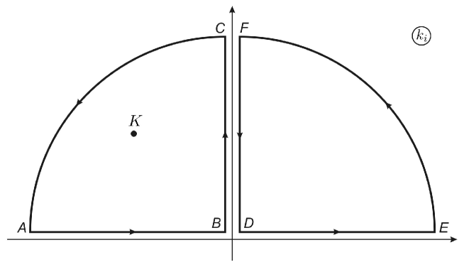
Figure 1: To calculation of integrals standing in equations (17) and (18)

in Eq.(12) can be rewritten as follows:

$$\begin{split}\int\limits_{-\infty}^{+\infty}\frac{f(k)}{k-K}{\rm d}k\equiv\int\limits_{AB}\frac{f(k)}{k-K}{\rm d}k+\int\limits_{DE}\frac{f(k)}{k-K}{\rm d}k\\ =\oint\limits_{ABC}\frac{f(k)}{k-K}{\rm d}k-\left[\int\limits_{BC}\frac{f(k)}{k-K}{\rm d}k+\int\limits_{CA}\frac{f(k)}{k-K}{\rm d}k\right]\\ +\oint\limits_{DEF}\frac{f(k)}{k-K}{\rm d}k-\left[\int\limits_{EF}\frac{f(k)}{k-K}{\rm d}k+\int\limits_{FD}\frac{f(k)}{k-K}{\rm d}k\right]\\ =\oint\limits_{ABC}\frac{f(k)}{k-K}{\rm d}k+\oint\limits_{DEF}\frac{f(k)}{k-K}{\rm d}k\\ -\left[\int\limits_{BC}\frac{f(k)}{k-K}{\rm d}k+\int\limits_{FD}\frac{f(k)}{k-K}{\rm d}k\right]-\left[\int\limits_{CA}\frac{f(k)}{k-K}{\rm d}k+\int\limits_{EF}\frac{f(k)}{k-K}{\rm d}k\right].\end{split}$$ (17)

With tending radiuses of the arcs $CA$ and $EF$ to infinity, both integrals in the last square brackets disappear. On the other hand, when both half-axes $BC$ and $FD$ tend one to another, one has $\int_{BC}=-\int_{FD}$, so that terms in the square brackets standing before are cancelled also. Moreover, the integral over the contour $DEF$ equals zero because this contour does not envelop any pole. As a result, we obtain

$$\int\limits_{-\infty}^{+\infty}\frac{f(k)}{k-K}{\rm d}k=\oint\limits_{ABC}\frac{f(k)}{k-K}{\rm d}k={\rm sgn}(\Im K)2\pi{\rm i}f(K)$$ (18)

where the last equality is due to the residue theorem.

Finally, making use of the Cauchy integral (18) yields the probability distribution (12) in the form

$$P\left(x_{1},x_{2}\right)=F_{1}^{\frac{2-\alpha}{\alpha-1}}P_{1}{\rm e}^{-{\rm i}\left(K_{1}x_{1}-\phi_{1}\right)}+F_{2}^{\frac{2-\alpha}{\alpha-1}}P_{2}{\rm e}^{-{\rm i}\left(K_{2}x_{2}-\phi_{2}\right)}$$ (19)

where one denotes

$$\begin{split}P_{1,2}&\equiv\frac{J_{2,1}\left(K_{1,2}\right)}{(\alpha-1)|g_{2,1}|^{\frac{\alpha}{2(\alpha-1)}}|m_{1,2}g_{1,2}|^{\frac{\alpha(3-\alpha)}{2(\alpha-1)}}},\\ \phi_{1,2}&\equiv\frac{3-\alpha}{\alpha-1}\varphi_{1,2}\left(\frac{\alpha}{2}\right)+\frac{\pi}{2}\frac{2-\alpha}{\alpha-1}\left[{\rm sgn}\left(\Im K_{1,2}\right)+2\theta\left(-\Re K_{1,2}\right)\right].\end{split}$$ (20)

3 Discussion

Analytical consideration developed in previous Section allowed us to obtain the probability distribution function (19) that describes behaviour of nonequilibrium steady-state stochastic system driven by the Lévy multiplicative noise with two degrees of freedom. Recently, we have studied conditions of the limit cycle creation in stochastic Lorenz-type systems driven by Gaussian noises [38]. Noise induced resonance was found analytically to appear in non-equilibrium steady state if the fastest variations displays a principle variable which is coupled with two different degrees of freedom or more. The condition of this resonance appearance is expressed formally in divergence of the probability distribution function being inverse proportional to an effective force type of (11) – when this force vanishes on a closed curve of phase plane, the system evolves along this cycle with diverging probability density.

In opposite to such a dependence, the distribution function (19) contains the effective force (11) in positive power $(2-\alpha)/(\alpha-1)$ only. To this end, we can conclude the Lévy flights suppress always a quasi-periodical motion related to the limit cycle. That is main result of our consideration. The corner stone of the difference between stochastic systems driven by the Lévy and Gaussian noises is that the Lévy variation $\Delta L\sim(\Delta t)^{1/\alpha}$ with the exponent $\alpha<2$ is negligible in comparison with the Gaussian variation $\Delta W\sim(\Delta t)^{1/2}$ in the $\Delta t\to 0$ limit.

It is interesting to note that above difference removes the problem of the calculus choice [1, 37]. This problem is known to be caused by irregularity of the time dependence $X(t)$ of stochastic variable (for the sake of simplicity, we consider one-dimensional case again). Hence, in the integral of equation of motion (1)

$$X(t)=\int\limits_{0}^{t}f\big{(}x(t^{\prime})\big{)}{\rm d}t^{\prime}+\int\limits_{L(0)}^{L(t)}g\big{(}x(\tilde{t^{\prime}})\big{)}{\rm d}L(t^{\prime})$$ (21)

we should take the noise amplitude $g\big{(}x(\tilde{t^{\prime}})\big{)}$ at the time moment

$$\tilde{t^{\prime}}=t^{\prime}+\lambda\Delta t^{\prime};\quad\lambda\in[0,1],\ \Delta t^{\prime}\to 0$$ (22)

that does not coincide with the integration time $t^{\prime}$ due to a parameter $\lambda\in[0,1]$ whose value fixes calculus choice (for example, the magnitude $\lambda=1/2$ relates to the Stratonovich case) [1, 37]. With accounting equations (22) and (1), one obtains

$$\begin{split}g\big{(}x(\tilde{t})\big{)}&\simeq g\big{(}x(t)\big{)}+\lambda g^{\prime}\big{(}x(t)\big{)}\Delta X(t)\\ &\simeq g\big{(}x(t)\big{)}+\lambda g^{\prime}\big{(}x(t)\big{)}f\big{(}x(t)\big{)}\Delta t+\lambda g^{\prime}\big{(}x(t)\big{)}g\big{(}x(t)\big{)}\Delta L(t)\end{split}$$ (23)

where primes denote differentiation over argument $x$. Being inserted into Eq.(21), the first term in the last line of Eq.(23) relates to usual case of the Îto calculus. Corresponding insertion of the second term gives an addition whose order $\Delta L\cdot\Delta t\sim(\Delta t)^{1+(1/\alpha)}\ll\Delta t$ is higher than one for the previous term (such a situation is inherent in the Gaussian case as well). Finally, after insertion of the last term of Eq.(23) the last integrand in Eq.(21) obtains an addition of order $(\Delta L)^{2}\sim(\Delta t)^{2/\alpha}$. In special case of the Gaussian noise $(\alpha=2)$, the order $2/\alpha$ of this addition coincides with the same in the first integrand of Eq.(21), that is resulted in addition $\lambda g(x)g^{\prime}(x)$ to the physical force $f(x)$. Principally different situation is realized for the Lévy stable process, when the index $\alpha<2$ and above addition should be suppressed in comparison with physical force because $(\Delta t)^{2/\alpha}\ll\Delta t$.

Appendix A. Derivation of Fokker-Planck equation for the Lévy multiplicative noises

Following to the line of Ref. [35], we start with consideration of one-dimensional Lévy process $X(t)$ whose Chapman-Kolmogorov equation

$$p(x,t+{\rm d}t|x_{0},t_{0})=\int{\rm d}y~{}p(x,t+{\rm d}t|y,t)p(y,t|x_{0},t_{0})$$ (A.1)

connects transition probabilities taken in intermediate positions $y$ related to time $t$. According to the definition

$$p(k,t+{\rm d}t|y,t):={\rm e}^{{\rm d}K_{X}(k,{\rm d}t|y,t)},$$ (A.2)

the inverse Fourier transform

$$p(x,t+{\rm d}t|y,t)=\int\frac{{\rm d}k}{2\pi}{\rm e}^{-{\rm i}k(x-y)}p(k,t+{\rm d}t|y,t)$$ (A.3)

is expressed in terms of the elementary cumulant ${\rm d}K_{X}(k,{\rm d}t|y,t)$ of the characteristic function of the stochastic process $X(t)$. Then, with using the ${\rm d}t\to 0$ limit and the identity

$$p(x,t|x_{0},t_{0})=\int{\rm d}y~{}p(y,t|x_{0},t_{0})\int\frac{{\rm d}k}{2\pi}{\rm e}^{-{\rm i}k(x-y)},$$ (A.4)

the equation (A.1) arrives at the chain of equalities:

$$\begin{split}p(x,t+{\rm d}t|x_{0},t_{0})-p(x,t|x_{0},t_{0})\\ =\int{\rm d}y~{}p(y,t|x_{0},t_{0})\int\frac{{\rm d}k}{2\pi}{\rm e}^{-{\rm i}k(x-y)}[{\rm e}^{{\rm d}K_{X}(k,{\rm d}t|y,t)}-1]\\ \simeq\int{\rm d}y~{}p(y,t|x_{0},t_{0})\int\frac{{\rm d}k}{2\pi}{\rm e}^{-{\rm i}k(x-y)}{\rm d}K_{X}(k,{\rm d}t|y,t)\\ =\int{\rm d}y~{}{\rm d}K_{X}(x-y,t)p(y,t|x_{0},t_{0})\equiv{\rm d}K_{X}(x,t)\star p(x,t|x_{0},t_{0}).\end{split}$$ (A.5)

Here, $\star$ denotes the convolution of the inverse Fourier transform

$${\rm d}K_{X}(x-y,t)=\int\frac{{\rm d}k}{2\pi}{\rm d}K_{X}(k,{\rm d}t|y,t){\rm e}^{-{\rm i}k(x-y)}.$$ (A.6)

As a result, with accounting the definition

$${\rm d}K_{X}(x,t):=\mathcal{L}(x){\rm d}t,$$ (A.7)

the equalities (A.5) yield the Fokker-Planck equation

$$\frac{\partial}{\partial t}p(x,t|x_{0},t_{0})=\mathcal{L}(x)\star p(x,t|x_{0},t_{0}).$$ (A.8)

To obtain the explicit form of the increment $\mathcal{L}(x)$ let us consider initially the Lévy process $L(t)$ itself. The elementary characteristic function related

$$\left<{\rm e}^{{\rm i}k{\rm d}L}\right>:={\rm e}^{{\rm d}K_{L}(k,{\rm d}t|y,t)}$$ (A.9)

is determined by the cumulant

$${\rm d}K_{L}(k,{\rm d}t|y,t):=\Lambda(k){\rm d}t$$ (A.10)

with the Lévy increment [39]

$$\Lambda(k)={\rm i}k\gamma-D|mk|^{\alpha}{\rm e}^{-{\rm i}\varphi(\alpha)}$$ (A.11)

where asymmetry angle $\varphi$ and modulus $m$ are determined by Eqs. (4). The elementary characteristic function of the principle process ${\rm d}X=f{\rm d}t+g{\rm d}L$ is written as follows:

$${\rm e}^{{\rm d}K_{X}(k,{\rm d}t|y,t)}:=\left<{\rm e}^{{\rm i}k{\rm d}X}\right>={\rm e}^{{\rm i}kf{\rm d}t}\left<{\rm e}^{{\rm i}(kg){\rm d}L}\right>={\rm e}^{{\rm i}kf{\rm d}t}{\rm e}^{{\rm d}K_{L}(gk,{\rm d}t|y,t)}$$ (A.12)

where Eq.(A.9) is taken into account. Similarly to the definition (A.10), the elementary cumulant

$${\rm d}K_{X}(k,{\rm d}t|y,t):=\mathcal{L}(k,x){\rm d}t$$ (A.13)

is determined by the increment

$$\mathcal{L}(k,x)={\rm i}kf(x)+\Lambda\big{(}g(x)k\big{)}$$ (A.14)

whose explicit form reads [35, 36]

$$\mathcal{L}(k,x)={\rm i}k\left[f(x)+\gamma g(x)\right]-|mg(x)k|^{\alpha}{\rm e}^{-{\rm i}\varphi(\alpha)}.$$ (A.15)

Hereafter, we renormalize the noise amplitude $g(x)$ to suppress the scale factor $D$.

The probability distribution function

$$P(x,t)=\int{\rm d}x_{0}~{}p(x,t|x_{0},t_{0})P(x_{0},t_{0})$$ (A.16)

is determined by the Fokker-Planck equation

$$\frac{\partial}{\partial t}P(x,t)=\mathcal{L}(x)\star P(x,t)\equiv\int{\rm d}y~{}\mathcal{L}(x-y,x)P(y,t)$$ (A.17)

following from Eq.(A.8). After using the Fourier transform

$$\widetilde{P}(k,t)\equiv\mathcal{F}\{P(y,t)\}(k,t)=\int{\rm d}y~{}P(y,t){\rm e}^{{\rm i}ky}$$ (A.18)

this equation takes the convenient form

$$\frac{\partial}{\partial t}\widetilde{P}(k,t)=\mathcal{L}(k,x)\widetilde{P}(k,t)$$ (A.19)

with the kernel (A.15). It is worthwhile to note this kernel, being the Fourier transform inverse to Eq.(A.6) with respect to the coordinate difference $x-y$, depends on the coordinate $x$ through both force $f(x)$ and multiplicative noise amplitude $g(x)$.

With accounting the relation

$$\frac{\partial^{\alpha}}{\partial|x|^{\alpha}}h(x)=-\mathcal{F}^{-1}\left\{|k|^{\alpha}\tilde{h}(k)\right\}$$ (A.20)

for the Riesz derivative with respect to an arbitrary function $h(x)$, Eqs. (A.19) and (A.15) arrive at the following form of the fractional Fokker-Planck equation [35, 36]

$$\begin{split}\frac{\partial}{\partial t}P(x,t)=&-\frac{\partial}{\partial x}\left[f(x)+\gamma g(x)\right]P(x,t)\\ &+\left[\frac{\partial^{\alpha}}{\partial|x|^{\alpha}}+\beta\tan\left(\frac{\pi\alpha}{2}\right)\frac{\partial}{\partial x}\frac{\partial^{\alpha-1}}{\partial|x|^{\alpha-1}}\right]|g(x)|^{\alpha}P(x,t).\end{split}$$ (A.21)

In symbolic form, many-dimensional generalization of this equation for a symmetric Lévy flight reads:

$$\frac{\partial}{\partial t}P(\vec{x},t)=-\nabla\left[\vec{f}(\vec{x})+\hat{g}(\vec{x})\cdot\vec{\gamma}\right]P(\vec{x},t)-\left[-\hat{\Delta}:\vec{g}(\vec{x})\vec{g}(\vec{x})\right]^{\alpha/2}P(\vec{x},t).$$ (A.22)

Here, every dot denotes the summation over indexes $i=1,2$ and the axes $x_{1}$, $x_{2}$ forming pseudovector $\vec{x}$ are chosen so that the noise amplitude matrix $\hat{g}$ takes the diagonal form $g_{ij}=g_{i}\delta_{ij}$ whose elements form the pseudovector $\vec{g}$. In the component form, one has the continuity equation

$$\frac{\partial}{\partial t}P(\vec{x},t)+\sum\limits_{i}\frac{\partial}{\partial x_{i}}J_{i}(\vec{x})=0$$ (A.23)

with the probability flux

$$J_{i}(\vec{x})=\left\{\left[f_{i}(\vec{x})+g_{i}(\vec{x})\gamma_{i}\right]+\frac{\partial^{\frac{\alpha}{2}-1}}{\partial x_{i}^{\frac{\alpha}{2}-1}}\sum\limits_{j}\left(-\frac{\partial}{\partial x_{j}}\right)^{\frac{\alpha}{2}}\left[g_{i}(\vec{x})g_{j}(\vec{x})\right]^{\frac{\alpha}{2}}\right\}P(\vec{x}).$$ (A.24)

In generalized case of non-symmetric Lévy flights, the Fourier transforms of the flux components are written in the explicit form

$$\begin{split}J_{1}&=\left\{\left(f_{1}+g_{1}\gamma_{1}\right)+{\rm i}|m_{1}g_{1}|^{\frac{\alpha}{2}}{\rm e}^{-{\rm i}\varphi_{1}\left(\frac{\alpha}{2}\right)}|k_{1}|^{\frac{\alpha}{2}-2}k_{1}\right.\\ &\left.\times\left[\left|m_{1}g_{1}k_{1}\right|^{\frac{\alpha}{2}}{\rm e}^{-{\rm i}\varphi_{1}\left(\frac{\alpha}{2}\right)}+\left|m_{2}g_{2}k_{2}\right|^{\frac{\alpha}{2}}{\rm e}^{-{\rm i}\varphi_{2}\left(\frac{\alpha}{2}\right)}\right]\right\}\widetilde{P},\\ J_{2}&=\left\{\left(f_{2}+g_{2}\gamma_{2}\right)+{\rm i}|m_{2}g_{2}|^{\frac{\alpha}{2}}{\rm e}^{-{\rm i}\varphi_{2}\left(\frac{\alpha}{2}\right)}|k_{2}|^{\frac{\alpha}{2}-2}k_{2}\right.\\ &\left.\times\left[\left|m_{1}g_{1}k_{1}\right|^{\frac{\alpha}{2}}{\rm e}^{-{\rm i}\varphi_{1}\left(\frac{\alpha}{2}\right)}+\left|m_{2}g_{2}k_{2}\right|^{\frac{\alpha}{2}}{\rm e}^{-{\rm i}\varphi_{2}\left(\frac{\alpha}{2}\right)}\right]\right\}\widetilde{P}\end{split}$$ (A.25)

where we use the asymmetry parameters (4).

Appendix B. Consideration of the Lévy processes within direct stochastic space

After inverse Fourier transformation, the components (7) and (8) of the stationary probability flux are written as follows:

$$\begin{split}\left\{\left(f_{1}+g_{1}\gamma_{1}\right)+\frac{\partial^{\frac{\alpha}{2}-1}}{\partial x_{1}^{\frac{\alpha}{2}-1}}\left[\left(-\frac{\partial}{\partial x_{1}}\right)^{\frac{\alpha}{2}}g_{1}^{\alpha}+\left(-\frac{\partial}{\partial x_{2}}\right)^{\frac{\alpha}{2}}\left(g_{1}g_{2}\right)^{\frac{\alpha}{2}}\right]\right\}P=J_{1}^{(0)}(x_{2}),\\ \left\{\left(f_{2}+g_{2}\gamma_{2}\right)+\frac{\partial^{\frac{\alpha}{2}-1}}{\partial x_{2}^{\frac{\alpha}{2}-1}}\left[\left(-\frac{\partial}{\partial x_{1}}\right)^{\frac{\alpha}{2}}\left(g_{2}g_{1}\right)^{\frac{\alpha}{2}}+\left(-\frac{\partial}{\partial x_{2}}\right)^{\frac{\alpha}{2}}g_{2}^{\alpha}\right]\right\}P=J_{2}^{(0)}(x_{1}).\end{split}$$

Acting by the $g_{2}^{\frac{\alpha}{2}}\frac{\partial^{\frac{\alpha}{2}-1}}{\partial x_{2}^{\frac{\alpha}{2}-1}}$ operator on the first of these equations and the $g_{1}^{\frac{\alpha}{2}}\frac{\partial^{\frac{\alpha}{2}-1}}{\partial x_{1}^{\frac{\alpha}{2}-1}}$ operator – on the second, one obtains

$$\begin{split}g_{2}^{\frac{\alpha}{2}}\frac{\partial^{\frac{\alpha}{2}-1}}{\partial x_{2}^{\frac{\alpha}{2}-1}}\frac{\partial^{\frac{\alpha}{2}-1}}{\partial x_{1}^{\frac{\alpha}{2}-1}}\left[\left(-\frac{\partial}{\partial x_{1}}\right)^{\frac{\alpha}{2}}g_{1}^{\alpha}+\left(-\frac{\partial}{\partial x_{2}}\right)^{\frac{\alpha}{2}}(g_{1}g_{2})^{\frac{\alpha}{2}}\right]P\\ =g_{2}^{\frac{\alpha}{2}}\frac{\partial^{\frac{\alpha}{2}-1}}{\partial x_{2}^{\frac{\alpha}{2}-1}}\left[J_{1}^{(0)}-\left(f_{1}+g_{1}\gamma_{1}\right)P\right],\\ g_{1}^{\frac{\alpha}{2}}\frac{\partial^{\frac{\alpha}{2}-1}}{\partial x_{1}^{\frac{\alpha}{2}-1}}\frac{\partial^{\frac{\alpha}{2}-1}}{\partial x_{2}^{\frac{\alpha}{2}-1}}\left[\left(-\frac{\partial}{\partial x_{1}}\right)^{\frac{\alpha}{2}}\left(g_{2}g_{1}\right)^{\frac{\alpha}{2}}+\left(-\frac{\partial}{\partial x_{2}}\right)^{\frac{\alpha}{2}}g_{2}^{\alpha}\right]P\\ =g_{1}^{\frac{\alpha}{2}}\frac{\partial^{\frac{\alpha}{2}-1}}{\partial x_{1}^{\frac{\alpha}{2}-1}}\left[J_{2}^{(0)}-\left(f_{2}+g_{2}\gamma_{2}\right)P\right].\end{split}$$ (B.1)

Subtracting above equalities term by term, one arrives at the fractional differential equation

$$\begin{split}\left[\left(f_{1}+g_{1}\gamma_{1}\right)g_{2}^{\frac{\alpha}{2}}\frac{\partial^{\frac{\alpha}{2}-1}}{\partial x_{2}^{\frac{\alpha}{2}-1}}-\left(f_{2}+g_{2}\gamma_{2}\right)g_{1}^{\frac{\alpha}{2}}\frac{\partial^{\frac{\alpha}{2}-1}}{\partial x_{1}^{\frac{\alpha}{2}-1}}\right]P+G\left(x_{1},x_{2}\right)P\\ =g_{2}^{\frac{\alpha}{2}}\frac{\partial^{\frac{\alpha}{2}-1}}{\partial x_{2}^{\frac{\alpha}{2}-1}}J_{1}^{(0)}\left(x_{2}\right)-g_{1}^{\frac{\alpha}{2}}\frac{\partial^{\frac{\alpha}{2}-1}}{\partial x_{1}^{\frac{\alpha}{2}-1}}J_{2}^{(0)}\left(x_{1}\right)\end{split}$$ (B.2)

where one denotes the function

$$\begin{split}G\left(x_{1},x_{2}\right)\equiv g_{2}^{\frac{\alpha}{2}}\frac{\partial^{\frac{\alpha}{2}-1}}{\partial x_{2}^{\frac{\alpha}{2}-1}}\frac{\partial^{\frac{\alpha}{2}-1}}{\partial x_{1}^{\frac{\alpha}{2}-1}}\left[\left(-\frac{\partial}{\partial x_{1}}\right)^{\frac{\alpha}{2}}g_{1}^{\alpha}+\left(-\frac{\partial}{\partial x_{2}}\right)^{\frac{\alpha}{2}}(g_{1}g_{2})^{\frac{\alpha}{2}}\right]\\ -g_{1}^{\frac{\alpha}{2}}\frac{\partial^{\frac{\alpha}{2}-1}}{\partial x_{1}^{\frac{\alpha}{2}-1}}\frac{\partial^{\frac{\alpha}{2}-1}}{\partial x_{2}^{\frac{\alpha}{2}-1}}\left[\left(-\frac{\partial}{\partial x_{1}}\right)^{\frac{\alpha}{2}}\left(g_{2}g_{1}\right)^{\frac{\alpha}{2}}+\left(-\frac{\partial}{\partial x_{2}}\right)^{\frac{\alpha}{2}}g_{2}^{\alpha}\right]\\ +\left[g_{2}^{\frac{\alpha}{2}}\frac{\partial^{\frac{\alpha}{2}-1}}{\partial x_{2}^{\frac{\alpha}{2}-1}}\left(f_{1}+g_{1}\gamma_{1}\right)-g_{1}^{\frac{\alpha}{2}}\frac{\partial^{\frac{\alpha}{2}-1}}{\partial x_{1}^{\frac{\alpha}{2}-1}}\left(f_{2}+g_{2}\gamma_{2}\right)\right].\end{split}$$ (B.3)

For the Gauss processes $(\alpha=2)$, the differential equation (B.2) is reduced to the algebraic one to give the probability distribution function that has been found in our previous work [38]. However, in general case $\alpha\leq 2$, solution of the fractional differential equation (B.2) arrives at a complicated problem, so that we are obliged to use the Fourier representation in Section 2.

It is worthwhile to note finally the consistency condition (9) takes the form

$$\begin{split}\left[\frac{\partial}{\partial x_{1}}\left(f_{1}+g_{1}\gamma_{1}\right)-\left(-\frac{\partial}{\partial x_{1}}\right)^{\alpha}|g_{1}|^{\alpha}\right]J_{2}^{(0)}(x_{1})\\ =\left[\frac{\partial}{\partial x_{2}}\left(f_{2}+g_{2}\gamma_{2}\right)-\left(-\frac{\partial}{\partial x_{2}}\right)^{\alpha}|g_{2}|^{\alpha}\right]J_{1}^{(0)}(x_{2})\end{split}$$ (B.4)

within the inverse Fourier representation where one takes $\varphi_{i}=0$ and $m_{i}=1$, for the simplicity. The equation (B.4) connects explicitly the probability flux components $J_{2,1}(x_{1,2})$, being arbitrary functions, with given dependencies of both forces $f_{1}(x_{1},x_{2})$, $f_{2}(x_{1},x_{2})$ and multiplicative amplitudes $g_{1}(x_{1},x_{2})$, $g_{2}(x_{1},x_{2})$, respectively.

References

• [1] H. Horsthemke, R. Lefever, Noise Induced Transitions, Springer-Verlag, Berlin, 1984.
• [2] P. Reimann, Brownian motors: noisy transport far from equilibrium, Phys. Rep. 361 (2002) 57 -265.
• [3] C. Van den Broeck, J.M.R. Parrondo, R. Toral, Noise-Induced Nonequilibrium Phase Transition, Phys. Rev. Lett. 73 (1994) 3395–3398; Mean field model for spatially extended systems in the presence of multiplicative noise, Phys. Rev. E 49 (1994) 2639–2643.
• [4] A.I. Olemskoi, D.O. Kharchenko, I.A. Knyaz’, Phase transitions induced by noise cross-correlations, Phys. Rev. E 71 (2005) 041101.
• [5] R. Benzi, A. Sutera, A. Vulpiani, The mechanism of stochastic resonance, J. Phys. A: Math. Gen. 14 (1981) L453–L457.
• [6] L. Gammaitoni, P. Hänggi, P. Jung, F. Marchesoni, Stochastic resonance, Rev. Mod. Phys. 70 (1998) 223–287.
• [7] J. Buceta, M. Ibaes, J.M. Sancho, Katja Lindenberg, Noise-driven mechanism for pattern formation, Phys. Rev. E 67 (2003) 021113.
• [8] M.C. Cross, P.C. Hohenberg, Pattern formation outside of equilibrium, Rev. Mod. Phys. 65 (1993) 851–1112.
• [9] F. Julicher, A. Ajdari, J. Prost, Modeling molecular motors, Rev. Mod. Phys. 69 (1997) 1269–1282.
• [10] F. Sagués, J.M. Sancho, J. Garcia-Ojalv, Spatiotemporal order out of noise, Rev. Mod. Phys. 79 (2007) 829–883.
• [11] R.L. Kautz, Chaos, thermal noise in the rf-biased Josephson junction, J. Appl. Phys. 58 (1985) 424–440.
• [12] F. Arecchi, R. Badii, A. Politi, Generalized multistability and noise-induced jumps in a nonlinear dynamical system, Phys. Rev. A 32 (1985) 402–408.
• [13] J.B. Gao, Wen-wen Tung, Nageswara Rao, Noise-Induced Hopf-Bifurcation-Type Sequence and Transition to Chaos in the Lorenz Equations, Phys. Rev. Lett. 89 (2002) 254101.
• [14] Omar Osenda, Carlos B. Briozzo, Manuel O. Caceres, Stochastic Lorenz model for periodically driven Rayleigh-Be’nard convection, Phys. Rev. E. 55 (1997) R3824–R3827.
• [15] D. Alonso, A.J. McKane, M. Pascual, Stochastic amplification in epidemics, J. R. Soc. Interface 4 (2007) 575–582.
• [16] M. Simoes, M.M. Telo da Gama, A. Nunes, Stochastic fluctuations in epidemics on networks, J. R. Soc. Interface 5 (2008) 555–566.
• [17] R. Kuske, L.F. Gordillo, P. Greenwood, Sustained oscillations via coherence resonance in SIR, J. Theor. Biol. 245 (2007) 459–469.
• [18] A.J. McKane, T.J. Newman, Predator-Prey Cycles from Resonant Amplification of Demographic Stochasticity, Phys. Rev. Lett. 94 (2005) 218102.
• [19] M. Pineda-Krch, H.J. Blok, U. Dieckmann, M. Doebeli, A tale of two cycles Distinguishing between true limit cycles and quasi-cycles in finite predator-prey populations, Oikos 116 (2007) 53–64.
• [20] M.S. de la Lama, I.G. Szendro, J.R. Iglesias, H.S. Wio, Van Kampen’s expansion approach in an opinion formation model, Eur. Phys. J. B 51 (2006) 435–442.
• [21] D. Gonze, J. Halloy, P. Gaspard, Biochemical clocks and molecular noise: Theoretical study of robustness factors, J. Chem. Phys. 116 (2002) 10997–11010.
• [22] A.J. McKane, J.D. Nagy, T.J. Newman, M.O. Stefanini, Amplified Biochemical Oscillations in Cellular Systems, J. Stat. Phys. 128 (2007) 165–191.
• [23] M. Scott, B. Ingalls, M. Kaern, Estimations of intrinsic and extrinsic noise in models of nonlinear genetic networks, Chaos 16 (2006) 026107.
• [24] E. Ben-Naim, P.L. Krapivsky, Finite-size fluctuations in interacting particle systems, Phys. Rev. E 69 (2004) 046113.
• [25] B.D. Hassard, N.D. Kazarinoff, Y.-H. Wan, Theory and Applications of Hopf Bifurcation, Cambridge University Press, Cambridge, 1981.
• [26] R. Grimshaw, Nonlinear Ordinary Differential Equations, Blackwell, Oxford, 1990.
• [27] M.S. Bartlett, Measles periodicity and community size, J. R. Stat. Soc. A 120 (1957) 48–70.
• [28] A.J. McKane, T.J. Newman, Predator-Prey Cycles from Resonant Amplification of Demographic Stochasticity, Phys. Rev. Let. 94 (2005) 218102.
• [29] A. Pikovsky, J. Kurths, Coherence Resonance in a Noise-Driven Excitable System, Phys. Rev. Let. 78 (1997) 775–778.
• [30] B. Lindner, L. Schimansky-Geier, Coherence and stochastic resonance in a two-state system, Phys. Rev. E 61 (2000) 6103–6110.
• [31] A. Neiman, P.I. Saparin, L. Stone, Coherence resonance at noisy precursors of bifurcations in nonlinear dynamical systems, Phys. Rev. E 56 (1997) 270–273.
• [32] H. Gang, T. Ditzinger, C.Z. Ning, H. Haken, Stochastic resonance without external periodic force, Phys. Rev. Let. 71 (1993) 807–810.
• [33] A.A. Dubkov, B. Spagnolo, V.V. Uchaikin, Lévy Flight Superdiffusion: An Introduction, Intern. Journ. of Bifurcation and Chaos 18 No. 9 (2008) 2649–2672.
• [34] A. Ichiki, M. Shiino, Phase transitions driven by Lévy stable noise: exact solutions and stability analysis of nonlinear fractional Fokker-Planck equations, arXiv:cond-mat.stat-mech/0907.3782v1.
• [35] D. Schertzer, M. Larchev$\hat{\rm e}$que, J. Duan, V.V. Yanovsky, S. Lovejoy, Fractional Fokker-Planck equation for nonlinear stochastic differential equations driven by non-Gaussian Lévy stable noise, J. Math. Phys: Math. Gen. 41 (2001) 200–212.
• [36] S.I. Denisov, W. Horsthemke, P. Hänggi, Generalized Fokker-Planck equation: Derivation and exact solutions, Eur. Phys. J. B 68 (2009) 567 -575.
• [37] H. Risken, The Fokker-Planck Equation, Springer-Verlag, Berlin, 1984.
• [38] I.A. Shuda, S.S. Borysov, A.I. Olemskoi, Noise-induced oscillations in non-equilibrium steady state systems, Physica Scripta 79 (2009) 065001.
• [39] P. Lévy, Theorie de l’addition des variables Aléatoires, Gauthier-Villars, Paris, 1937.