The Projector Augmented-wave Method

Abstract

The purpose of this text is to give a self-contained description of the basic theory of the projector augmented-wave (PAW) method, as well as most of the details required to make the method work in practice. These two topics are covered in the first two sections, while the last is dedicated to examples of how to apply the PAW transformation when extracting non-standard quantities from a density-functional theory (DFT) calculation.

The formalism is based on Blöchl’s original formulation of PAW [1], and the notation and extensions follow those used and implemented in the gpaw[2] code.

1 Formalism

By the requirement of orthogonality, DFT wave functions have very sharp features close to the nuclei, as all the states are non-zero in this region. Further out only the valence states are non-zero, resulting in much smoother wave functions in this interstitial region. The oscillatory behavior in the core regions, requires a very large set of plane waves, or equivalently a very fine grid, to be described correctly. One way of solving this problem is the use of pseudopotentials in which the collective system of nuclei and core electrons are described by an effective, much smoother, potential. The KS equations are then solved for the valence electrons only. The pseudopotentials are constructed such that the correct scattering potential is obtained beyond a certain radius from the core. This method reduces the number of wave functions to be calculated, since the pseudo potentials only have to be calculated and tabulated once for each type of atom, so that only calculations on the valence states are needed. It justifies the neglect of relativistic effects in the KS equations, since the valence electrons are non-relativistic (the pseudopotentials describing core states are of course constructed with full consideration of relativistic effects). The technique also removes the unwanted singular behavior of the ionic potential at the lattice points.

The drawback of the method is that all information on the full wave function close to the nuclei is lost. This can influence the calculation of certain properties, such as hyperfine parameters, and electric field gradients. Another problem is that one has no before hand knowledge of when the approximation yields reliable results.

A different approach is the augmented-plane-wave method (APW), in which space is divided into atom-centered augmentation spheres inside which the wave functions are taken as some atom-like partial waves, and a bonding region outside the spheres, where some envelope functions are defined. The partial waves and envelope functions are then matched at the boundaries of the spheres.

A more general approach is the projector augmented wave method (PAW) presented here, which offers APW as a special case[3], and the pseudopotential method as a well defined approximation[4]. The PAW method was first proposed by Bl chl in 1994[1].

1.1 The Transformation Operator

The features of the wave functions, are very different in different regions of space. In the bonding region it is smooth, but near the nuclei it displays rapid oscillations, which are very demanding on the numerical representation of the wave functions. To address this problem, we seek a linear transformation $\hat{\mathcal{T}}$ which takes us from an auxiliary smooth wave function $|\tilde{\psi}_{n}\rangle$ to the true all electron Kohn-Sham single particle wave function $|\psi_{n}\rangle$

$$|\psi_{n}\rangle=\hat{\mathcal{T}}|\tilde{\psi}_{n}\rangle,$$ (1)

where $n$ is the quantum state label, containing a $\mathbf{k}$ index, a band index, and a spin index.

This transformation yields the transformed KS equations

$$\hat{\mathcal{T}}^{\dagger}\widehat{H}\hat{\mathcal{T}}|\tilde{\psi}_{n}\rangle=\epsilon_{n}\hat{\mathcal{T}}^{\dagger}\hat{\mathcal{T}}|\tilde{\psi}_{n}\rangle,$$ (2)

which needs to be solved instead of the usual KS equation. Now we need to define $\hat{\mathcal{T}}$ in a suitable way, such that the auxiliary wave functions obtained from solving (2) becomes smooth.

Since the true wave functions are already smooth at a certain minimum distance from the core, $\hat{\mathcal{T}}$ should only modify the wave function close to the nuclei. We thus define

$$\hat{\mathcal{T}}=1+\sum_{a}\hat{\mathcal{T}}^{a},$$ (3)

where $a$ is an atom index, and the atom-centered transformation, $\hat{\mathcal{T}}^{a}$, has no effect outside a certain atom-specific augmentation region $|\mathbf{r}-\mathbf{R}^{a}|<r_{c}^{a}$. The cut-off radii, $r_{c}^{a}$ should be chosen such that there is no overlap of the augmentation spheres.

Inside the augmentation spheres, we expand the true wave function in the partial waves $\phi_{i}^{a}$, and for each of these partial waves, we define a corresponding auxiliary smooth partial wave $\tilde{\phi}_{i}^{a}$, and require that

$$|\phi_{i}^{a}\rangle=(1+\hat{\mathcal{T}}^{a})|\tilde{\phi}_{i}^{a}\rangle\quad\Leftrightarrow\quad\hat{\mathcal{T}}^{a}|\tilde{\phi}_{i}^{a}\rangle=|\phi_{i}^{a}\rangle-|\tilde{\phi}_{i}^{a}\rangle$$ (4)

for all $i,a$. This completely defines $\hat{\mathcal{T}}$, given $\phi$ and $\tilde{\phi}$.

Since $\hat{\mathcal{T}}^{a}$ should do nothing outside the augmentation sphere, we see from (4) that we must require the partial wave and its smooth counterpart to be identical outside the augmentation sphere

$$\forall a,\quad\phi_{i}^{a}(\mathbf{r})=\tilde{\phi}_{i}^{a}(\mathbf{r})\text{, for }r>r_{c}^{a}$$

where $\phi_{i}^{a}(\mathbf{r})=\langle\mathbf{r}|\phi_{i}^{a}\rangle$ and likewise for $\tilde{\phi}_{i}^{a}$.

If the smooth partial waves form a complete set inside the augmentation sphere, we can formally expand the smooth all electron wave functions as

$$|\tilde{\psi}_{n}\rangle=\sum_{i}P_{ni}^{a}|\tilde{\phi}_{i}^{a}\rangle\text{, for }|\mathbf{r}-\mathbf{R}^{a}|<r_{c}^{a}$$ (5)

where $P_{ni}^{a}$ are some, for now, undetermined expansion coefficients.

Since $|\phi_{i}^{a}\rangle=\hat{\mathcal{T}}|\tilde{\phi}_{i}^{a}\rangle$ we see that the expansion

$$|\psi_{n}\rangle=\hat{\mathcal{T}}|\tilde{\psi}_{n}\rangle=\sum_{i}P_{ni}^{a}|\phi_{i}^{a}\rangle\text{, for }|\mathbf{r}-\mathbf{R}^{a}|<r_{c}^{a}$$ (6)

has identical expansion coefficients, $P_{ni}^{a}$.

As we require $\hat{\mathcal{T}}$ to be linear, the coefficients $P_{ni}^{a}$ must be linear functionals of $|\tilde{\psi}_{n}\rangle$, i.e.

$$P_{ni}^{a}=\langle\tilde{p}_{i}^{a}|\tilde{\psi}_{n}\rangle=\int d\mathbf{r}\tilde{p}_{i}^{a*}(\mathbf{r}-\mathbf{R}^{a})\tilde{\psi}_{n}(\mathbf{r}),$$ (7)

where $|\tilde{p}_{i}^{a}\rangle$ are some fixed functions termed smooth projector functions.

As there is no overlap between the augmentation spheres, we expect the one center expansion of the smooth all electron wave function, $|\tilde{\psi}^{a}_{n}\rangle=\sum_{i}|\tilde{\phi}_{i}^{a}\rangle\langle\tilde{p}_{i}^{a}|\tilde{\psi}_{n}\rangle$ to reduce to $|\tilde{\psi}_{n}\rangle$ itself inside the augmentation sphere defined by $a$. Thus, the smooth projector functions must satisfy

$$\sum_{i}|\tilde{\phi}_{i}^{a}\rangle\langle\tilde{p}_{i}^{a}|=1$$ (8)

inside each augmentation sphere. This also implies that

$$\langle\tilde{p}_{i_{1}}^{a}|\tilde{\phi}_{i_{2}}^{a}\rangle=\delta_{i_{1},i_{2}}\text{~{}, for }|\mathbf{r}-\mathbf{R}^{a}|<r_{c}^{a}$$ (9)

i.e. the projector functions should be orthonormal to the smooth partial waves inside the augmentation sphere. There are no restrictions on $\tilde{p}_{i}^{a}$ outside the augmentation spheres, so for convenience we might as well define them as local functions, i.e. $\tilde{p}_{i}^{a}(\mathbf{r})=0$ for $r>r_{c}^{a}$.

Note that the completeness relation (8) is equivalent to the requirement that $\tilde{p}_{i}^{a}$ should produce the correct expansion coefficients of (5)-(6), while (9) is merely an implication of this restriction. Translating (8) to an explicit restriction on the projector functions is a rather involved procedure, but according to Bl chl, [1], the most general form of the projector functions is:

$$\langle\tilde{p}_{i}^{a}|=\sum_{j}(\{\langle f_{k}^{a}|\tilde{\phi}_{l}^{a}\rangle\})^{-1}_{ij}\langle f_{j}^{a}|,$$ (10)

where $|f_{j}^{a}\rangle$ is any set of linearly independent functions. The projector functions will be localized if the functions $|f_{j}^{a}\rangle$ are localized.

Using the completeness relation (8), we see that

$$\hat{\mathcal{T}}^{a}=\sum_{i}\hat{\mathcal{T}}^{a}|\tilde{\phi}_{i}^{a}\rangle\langle\tilde{p}_{i}^{a}|=\sum_{i}\big{(}|\phi_{i}^{a}\rangle-|\tilde{\phi}_{i}^{a}\rangle\big{)}\langle\tilde{p}_{i}^{a}|,$$

where the first equality is true in all of space, since (8) holds inside the augmentation spheres and outside $\hat{\mathcal{T}}^{a}$ is zero, so anything can be multiplied with it. The second equality is due to (4) (remember that $|\phi_{i}^{a}\rangle-|\tilde{\phi}_{i}^{a}\rangle=0$ outside the augmentation sphere). Thus we conclude that

$$\hat{\mathcal{T}}=1+\sum_{a}\sum_{i}\big{(}|\phi_{i}^{a}\rangle-|\tilde{\phi}_{i}^{a}\rangle\big{)}\langle\tilde{p}_{i}^{a}|.$$ (11)

To summarize, we obtain the all electron KS wave function $\psi_{n}(\mathbf{r})=\langle\mathbf{r}|\psi_{n}\rangle$ from the transformation

$$\psi_{n}(\mathbf{r})=\tilde{\psi}_{n}(\mathbf{r})+\sum_{a}\sum_{i}\big{(}\phi_{i}^{a}(\mathbf{r})-\tilde{\phi}_{i}^{a}(\mathbf{r})\big{)}\langle\tilde{p}_{i}^{a}|\tilde{\psi}_{n}\rangle,$$ (12)

where the smooth (and thereby numerically convenient) auxiliary wave function $\tilde{\psi}_{n}(\mathbf{r})$ is obtained by solving the eigenvalue equation (2).

The transformation (12) is expressed in terms of the three components: a) the partial waves $\phi_{i}^{a}(\mathbf{r})$, b) the smooth partial waves $\tilde{\phi}_{i}^{a}(\mathbf{r})$, and c) the smooth projector functions $\tilde{p}_{i}^{a}(\mathbf{r})$.

The restriction on the choice of these sets of functions are: a) Since the partial- and smooth partial wave functions are used to expand the all electron wave functions, i.e. are used as atom-specific basis sets, these must be complete (inside the augmentation spheres). b) the smooth projector functions must satisfy (8), i.e. be constructed according to (10). All remaining degrees of freedom are used to make the expansions converge as fast as possible, and to make the functions termed ‘smooth’, as smooth as possible. For a specific choice of these sets of functions, see section 2.2. As the partial- and smooth partial waves are merely used as basis sets they can be chosen as real functions (any imaginary parts of the functions they expand, are then introduced through the complex expansion coefficients $P_{ni}^{a}$). In the remainder of this document $\phi$ and $\tilde{\phi}$ will be assumed real.

Note that the sets of functions needed to define the transformation are system independent, and as such they can conveniently be pre-calculated and tabulated for each element of the periodic table.

For future convenience, we also define the one center expansions

$$\psi_{n}^{a}(\mathbf{r}) =\sum_{i}\phi_{i}^{a}(\mathbf{r})\langle\tilde{p}_{i}^{a}|\tilde{\psi}_{n}\rangle,$$ (13a)

$$\tilde{\psi}_{n}^{a}(\mathbf{r}) =\sum_{i}\tilde{\phi}_{i}^{a}(\mathbf{r})\langle\tilde{p}_{i}^{a}|\tilde{\psi}_{n}\rangle.$$ (13b)

In terms of these, the all electron KS wave function is

$$\psi_{n}(\mathbf{r})=\tilde{\psi}_{n}(\mathbf{r})+\sum_{a}\big{(}\psi_{n}^{a}(\mathbf{r}-\mathbf{R}^{a})-\tilde{\psi}_{n}^{a}(\mathbf{r}-\mathbf{R}^{a})\big{)}.$$ (14)

So what have we achieved by this transformation? The trouble of the original KS wave functions, was that they displayed rapid oscillations in some parts of space, and smooth behavior in other parts of space. By the decomposition (12) we have separated the original wave functions into auxiliary wave functions which are smooth everywhere and a contribution which contains rapid oscillations, but only contributes in certain, small, areas of space. This decomposition is shown on the front page for the hydrogen molecule. Having separated the different types of waves, these can be treated individually. The localized atom centered parts, are indicated by a superscript $a$, and can efficiently be represented on atom centered radial grids. Smooth functions are indicated by a tilde ~. The delocalized parts (no superscript $a$) are all smooth, and can thus be represented on coarse Fourier- or real space grids.

1.2 The Frozen Core Approximation

In the frozen core approximation, it is assumed that the core states are naturally localized within the augmentation spheres, and that the core states of the isolated atoms are not changed by the formation of molecules or solids. Thus the core KS states are identical to the atomic core states

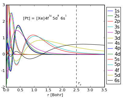
Figure 1: The core states of Platinum

$$|\psi^{c}_{n}\rangle=|\phi_{\alpha}^{a,\text{core}}\rangle,$$

where the index $n$ on the left hand site refers to both a specific atom, $a$, and an atomic state, $\alpha$.

In this approximation only valence states are included in the expansions of $|\psi_{n}\rangle$, (6), and $|\tilde{\psi}_{n}\rangle$, (5).

Figure 1, shows the atomic states of Platinum in its ground state, obtained with an atomic DFT program at an LDA level, using spherical averaging, i.e. a spin-compensated calculation, assuming the degenerate occupation 9/10 of all 5d states, and both of the 6s states half filled. It is seen that at the typical length of atomic interaction (the indicated cut-off $r_{c}=2.5$ Bohr is approximately half the inter-atomic distance in bulk Pt), only the 5d and 6s states are non-zero.

1.3 Expectation Values

The expectation value of an operator $\widehat{O}$ is, within the frozen core approximation, given by

$$\langle\widehat{O}\rangle=\sum_{n}^{\text{val}}f_{n}\langle\psi_{n}|\widehat{O}|\psi_{n}\rangle+\sum_{a}\sum_{\alpha}^{\text{core}}\langle\phi_{\alpha}^{a,\text{core}}|\widehat{O}|\phi_{\alpha}^{a,\text{core}}\rangle.$$ (15)

Using that $\langle\psi_{n}|\widehat{O}|\psi_{n}\rangle=\langle\tilde{\psi}_{n}|\hat{\mathcal{T}}^{\dagger}\widehat{O}\hat{\mathcal{T}}|\tilde{\psi}_{n}\rangle$, and skipping the state index for notational convenience, we see that

$$\begin{split}\langle\psi|\widehat{O}|\psi\rangle&=\langle\tilde{\psi}+\sum_{a}(\psi^{a}-\tilde{\psi}^{a})|\widehat{O}|\tilde{\psi}+\sum_{a}(\psi^{a}-\tilde{\psi}^{a})\rangle\\ &=\langle\tilde{\psi}|\widehat{O}|\tilde{\psi}\rangle+\sum_{aa^{\prime}}\langle\psi^{a}-\tilde{\psi}^{a}|\widehat{O}|\psi^{a^{\prime}}-\tilde{\psi}^{a^{\prime}}\rangle+\sum_{a}\left(\langle\tilde{\psi}|\widehat{O}|\psi^{a}-\tilde{\psi}^{a}\rangle+\langle\psi^{a}-\tilde{\psi}^{a}|\widehat{O}|\tilde{\psi}\rangle\right)\\ &=\langle\tilde{\psi}|\widehat{O}|\tilde{\psi}\rangle+\sum_{a}\left(\langle\psi^{a}|\widehat{O}|\psi^{a}\rangle-\langle\tilde{\psi}^{a}|\widehat{O}|\tilde{\psi}^{a}\rangle\right)\\ &\hskip 48.0pt+\sum_{a}\left(\langle\psi^{a}-\tilde{\psi}^{a}|\widehat{O}|\tilde{\psi}-\tilde{\psi}^{a}\rangle+\langle\tilde{\psi}-\tilde{\psi}^{a}|\widehat{O}|\psi^{a}-\tilde{\psi}^{a}\rangle\right)\\ &\hskip 48.0pt+\sum_{a\neq a^{\prime}}\langle\psi^{a}-\tilde{\psi}^{a}|\widehat{O}|\psi^{a^{\prime}}-\tilde{\psi}^{a^{\prime}}\rangle.\end{split}$$ (16)

For local operators the last two lines does not contribute. The first line, because $|\psi^{a}-\tilde{\psi}^{a}\rangle$ is only non-zero inside the spheres, while $|\tilde{\psi}-\tilde{\psi}^{a}\rangle$ is only non-zero outside the spheres. The second line simply because $|\psi^{a}-\tilde{\psi}^{a}\rangle$ is zero outside the spheres, so two such states centered on different nuclei have no overlap (provided that the augmentation spheres do not overlap).

Reintroducing the partial waves in the one-center expansions, we see that

$$\sum_{n}^{\text{val}}f_{n}\langle\psi_{n}^{a}|\widehat{O}|\psi_{n}^{a}\rangle=\sum_{n}^{\text{val}}f_{n}\sum_{i_{1}i_{2}}\langle\phi_{i_{1}}^{a}P^{a}_{ni_{1}}|\widehat{O}|\phi_{i_{2}}^{a}P_{ni_{2}}^{a}\rangle=\sum_{i_{1}i_{2}}\langle\phi_{i_{1}}^{a}|\widehat{O}|\phi_{i_{2}}^{a}\rangle\sum_{n}^{\text{val}}f_{n}P_{ni_{1}}^{a*}P_{ni_{2}}^{a},$$ (17)

and likewise for the smooth waves.

Introducing the Hermitian one-center density matrix

$$D_{i_{1}i_{2}}^{a}=\sum_{n}f_{n}P_{ni_{1}}^{a*}P_{ni_{2}}^{a}=\sum_{n}f_{n}\langle\tilde{\psi}_{n}|\tilde{p}_{i_{1}}^{a}\rangle\langle\tilde{p}_{i_{2}}^{a}|\tilde{\psi}_{n}\rangle.$$ (18)

We conclude that for any local operator $\widehat{O}$, the expectation value is

$$\langle\widehat{O}\rangle=\sum_{n}^{\text{val}}f_{n}\langle\tilde{\psi}_{n}|\widehat{O}|\tilde{\psi}_{n}\rangle+\sum_{a}\sum_{i_{1}i_{2}}\left(\langle\phi_{i_{1}}^{a}|\widehat{O}|\phi_{i_{2}}^{a}\rangle-\langle\tilde{\phi}_{i_{1}}^{a}|\widehat{O}|\tilde{\phi}_{i_{2}}^{a}\rangle\right)D_{i_{1}i_{2}}^{a}+\sum_{a}\sum_{\alpha}^{\text{core}}\langle\phi_{\alpha}^{a,\text{core}}|\widehat{O}|\phi_{\alpha}^{a,\text{core}}\rangle.$$ (19)

1.4 Densities

The electron density is obviously a very important quantity in DFT, as all observables in principle are calculated as functionals of the density. In reality the kinetic energy is calculated as a functional of the orbitals, and some specific exchange-correlation functionals also rely on KS-orbitals rather then the density for their evaluation, but these are still implicit functionals of the density.

To obtain the electron density we need to determine the expectation value of the real-space projection operator $|\mathbf{r}\rangle\langle\mathbf{r}|$

$$n(\mathbf{r})=\sum_{n}f_{n}\langle\psi_{n}|\mathbf{r}\rangle\langle\mathbf{r}|\psi_{n}\rangle=\sum_{n}f_{n}|\psi_{n}(\mathbf{r})|^{2},$$ (20)

where $f_{n}$ are the occupation numbers.

As the real-space projection operator is obviously a local operator, we can use the results (19) of the previous section, and immediately arrive at

$$n(\mathbf{r})=\sum_{n}^{\text{val}}f_{n}|\tilde{\psi}_{n}|^{2}+\sum_{a}\sum_{i_{1}i_{2}}\left(\phi_{i_{1}}^{a}\phi_{i_{2}}^{a}-\tilde{\phi}_{i_{1}}^{a}\tilde{\phi}_{i_{2}}^{a}\right)D_{i_{1}i_{2}}^{a}+\sum_{a}\sum_{\alpha}^{\text{core}}|\phi_{\alpha}^{a,\text{core}}|^{2}.$$ (21)

To ensure that (21) reproduce the correct density even though some of the core states are not strictly localized within the augmentation spheres, a smooth core density, $\tilde{n}_{c}(\mathbf{r})$, is usually constructed, which is identical to the core density outside the augmentation sphere, and a smooth continuation inside. Thus the density is typically evaluated as

$$n(\mathbf{r})=\tilde{n}(\mathbf{r})+\sum_{a}\left(n^{a}(\mathbf{r})-\tilde{n}^{a}(\mathbf{r})\right),$$ (22)

where

$$\tilde{n}(\mathbf{r}) =\sum_{n}^{\text{val}}f_{n}|\tilde{\psi}_{n}(\mathbf{r})|^{2}+\tilde{n}_{c}(\mathbf{r})$$ (23a)

$$n^{a}(\mathbf{r}) =\sum_{i_{1}i_{2}}D_{i_{1}i_{2}}^{a}\phi_{i_{1}}^{a}(\mathbf{r})\phi_{i_{2}}^{a}(\mathbf{r})+n_{c}^{a}(\mathbf{r})$$ (23b)

$$\tilde{n}^{a}(\mathbf{r}) =\sum_{i_{1}i_{2}}D_{i_{1}i_{2}}^{a}\tilde{\phi}_{i_{1}}^{a}(\mathbf{r})\tilde{\phi}_{i_{2}}^{a}(\mathbf{r})+\tilde{n}_{c}^{a}(\mathbf{r})$$ (23c)

1.5 Total Energies

The total energy of the electronic system is given by:

$$E[n]=T_{s}[n]+U_{H}[n]+V_{ext}[n]+E_{xc}[n].$$ (24)

In this section, the usual energy expression above, is sought re-expressed in terms of the PAW quantities: the smooth waves and the auxiliary partial waves.

For the local and semi-local functionals, we can utilize (19), while the nonlocal parts needs more careful consideration.

1.5.1 The Semi-local Contributions

The kinetic energy functional $T_{s}=\sum_{n}f_{n}\langle\psi_{n}|-\frac{1}{2}\nabla^{2}|\psi_{n}\rangle$ is obviously a (semi-) local functional, so we can apply (19) and immediately arrive at:

$$\begin{split}T_{s}[\{\psi_{n}\}]&=\sum_{n}f_{n}\langle\psi_{n}|-\tfrac{1}{2}\nabla^{2}|\psi_{n}\rangle\\ &=\sum_{n}^{\text{val}}f_{n}\langle\tilde{\psi}_{n}|-\tfrac{1}{2}\nabla^{2}|\tilde{\psi}_{n}\rangle+\sum_{a}\left(T_{c}^{a}+\Delta T_{i_{1}i_{2}}^{a}D^{a}_{i_{1}i_{2}}\right),\end{split}$$ (25)

where

$$T_{c}^{a}=\sum_{\alpha}^{\text{core}}\langle\phi_{\alpha}^{a,\text{core}}|-\tfrac{1}{2}\nabla^{2}|\phi_{\alpha}^{a,\text{core}}\rangle\quad\text{and}\quad\Delta T_{i_{1}i_{2}}^{a}=\langle\phi_{i_{1}}^{a}|-\tfrac{1}{2}\nabla^{2}|\phi_{i_{2}}^{a}\rangle-\langle\tilde{\phi}_{i_{1}}^{a}|-\tfrac{1}{2}\nabla^{2}|\tilde{\phi}_{i_{2}}^{a}\rangle.$$ (26)

For LDA and GGA type exchange-correlation functionals, $E_{xc}$ is likewise, per definition, a semi-local functional, such that it can be expressed as

$$E_{xc}[n]=E_{xc}[\tilde{n}]+\sum_{a}\left(E_{xc}[n^{a}]-E_{xc}[\tilde{n}^{a}]\right).$$ (27)

By virtue of (23b)-(23c) we can consider the atomic corrections as functionals of the density matrix defined in (18), i.e.

$$E_{xc}[n]=E_{xc}[\tilde{n}]+\sum_{a}\Delta E_{xc}^{a}[\{D^{a}_{i_{1}i_{2}}\}],$$ (28)

where

$$\Delta E_{xc}^{a}[\{D^{a}_{i_{1}i_{2}}\}]=E_{xc}[n^{a}]-E_{xc}[\tilde{n}^{a}].$$ (29)

1.5.2 The Nonlocal Contributions

The Hartree term is both nonlinear and nonlocal, so more care needs to be taken when introducing the PAW transformation for this expression.

In the following we will assume that there is no ‘true’ external field, such that $V_{\text{ext}}[n]$ is only due to the static nuclei, i.e. it is a sum of the classical interaction of the electron density with the static ionic potential, and the electrostatic energy of the nuclei.

We define the total classical electrostatic energy functional as

$$\begin{split}E_{C}[n]&=U_{H}[n]+V_{\text{ext}}[n]=\frac{1}{2}((n))+(n|\textstyle\sum_{a}Z^{a})+\frac{1}{2}\sum_{a\neq a^{\prime}}(Z^{a}|Z^{a^{\prime}}),\end{split}$$ (30)

where the notation (f|g) indicates the Coulomb integral

$$(f|g)=\iint d\mathbf{r}d\mathbf{r}^{\prime}\frac{f^{*}(\mathbf{r})g(\mathbf{r}^{\prime})}{|\mathbf{r}-\mathbf{r}^{\prime}|}$$ (31)

and I have introduced the short hand notation $((f))=(f|f)$. In (30), $Z^{a}(\mathbf{r})$ is the charge density of the nucleus at atomic site $a$, which in the classical point approximation is given by

$$Z^{a}(\mathbf{r})=-\mathcal{Z}^{a}\delta(\mathbf{r}-\mathbf{R}^{a})$$ (32)

with $\mathcal{Z}^{a}$ being the atomic number of the nuclei. As the Hartree energy of a density with non-zero total charge is numerically inconvenient, we introduce the charge neutral total density

$$\rho(\mathbf{r})=n(\mathbf{r})+\sum_{a}Z^{a}(\mathbf{r})\quad(=n_{\text{electrons}}+n_{\text{nuclei}}).$$ (33)

In terms of this, the coulombic energy of the system can be expressed by

$$E_{C}[n]=U_{H}^{\prime}[\rho]=\frac{1}{2}((n+{\textstyle\sum_{a}Z^{a}}))^{\prime}$$ (34)

where the prime indicates that one should remember the self-interaction error of the nuclei introduced in the Hartree energy of the total density. This correction is obviously ill defined, and different schemes exist for making this correction. As it turns out, this correction is handled very naturally in the PAW formalism.

For now, we will focus on the term $((\rho))=((n+\textstyle\sum_{a}Z^{a}))$. If one where to directly include the expansion of $n(\mathbf{r})$ according to (22), one would get:

$$((n+\textstyle\sum_{a}Z^{a})) =((\tilde{n}+\textstyle\sum_{a}n^{a}-\tilde{n}^{a}+Z^{a}))$$

$$=((\tilde{n}))+\sum_{aa^{\prime}}(n^{a}-\tilde{n}^{a}+Z^{a}|n^{a^{\prime}}-\tilde{n}^{a^{\prime}}+Z^{a^{\prime}})+2\sum_{a}(\tilde{n}|n^{a}-\tilde{n}^{a}+Z^{a}),$$

where in the last expression, the first term is the Hartree energy of the smooth electron density, which is numerically problematic because of the nonzero total charge. The second term contains a double summation over all nuclei, which would scale badly with system size, and the last term involves integrations of densities represented on incompatible grids (remember that the one-center densities are represented on radial grids to capture the oscillatory behavior near the nuclei). This is clearly not a feasible procedure. To correct these problem we add and subtract some atom centered compensation charges $\tilde{Z}^{a}$:

$$((n+\textstyle\sum_{a}\tilde{Z}^{a}+\textstyle\sum_{a}\left[Z^{a}-\tilde{Z}^{a}\right]))=((\tilde{n}+\textstyle\sum_{a}\tilde{Z}^{a}))+\sum_{aa^{\prime}}(n^{a}-\tilde{n}^{a}+Z^{a}-\tilde{Z}^{a}|n^{a^{\prime}}-\tilde{n}^{a^{\prime}}+Z^{a^{\prime}}-\tilde{Z}^{a})\\ +2\sum_{a}(\tilde{n}+\textstyle\sum_{a^{\prime}}\tilde{Z}^{a^{\prime}}|n^{a}-\tilde{n}^{a}+Z^{a}-\tilde{Z}^{a}).$$

If we define $\tilde{Z}^{a}(\mathbf{r})$ in such a way that $n^{a}(\mathbf{r})-\tilde{n}^{a}(\mathbf{r})+Z^{a}(\mathbf{r})-\tilde{Z}^{a}(\mathbf{r})$ has no multipole moments, i.e.

$$\int d\mathbf{r}r^{l}Y_{L}(\widehat{\mathbf{r}-\mathbf{R}^{a}})(n^{a}-\tilde{n}^{a}+Z^{a}-\tilde{Z}^{a})=0$$ (35)

for all $a$, the potentials of these densities are zero outside their respective augmentation spheres ($L=(l,m)$ is a collective angular- and magnetic quantum number). Exploiting this feature, the Coulomb integral reduce to

$$((n+\textstyle\sum_{a}Z^{a})) =((\tilde{n}+\textstyle\sum_{a}\tilde{Z}^{a}))+\sum_{a}((n^{a}-\tilde{n}^{a}+Z^{a}-\tilde{Z}^{a}))+2\sum_{a}(\tilde{n}^{a}+\tilde{Z}^{a}|n^{a}-\tilde{n}^{a}+Z^{a}-\tilde{Z}^{a})$$

$$=((\tilde{n}+\textstyle\sum_{a}\tilde{Z}^{a}))+\sum_{a}\left(((n^{a}+Z^{a}))-((\tilde{n}^{a}+\tilde{Z}^{a}))\right)$$

where it has been used that inside the augmentation spheres $\tilde{n}=\tilde{n}^{a}$. In this expression, we have circumvented all of the previous problems. None of the terms correlates functions on different grids, there is only a single summation over the atomic sites, and furthermore the only thing that has to be evaluated in the full space is the Hartree energy of $\tilde{n}(\mathbf{r})+\sum_{a}\tilde{Z}^{a}(\mathbf{r})$ which is charge neutral (see eq. (42)).

Inserting the final expression in (30), we see that

$$\begin{split}E_{C}[n]&=\frac{1}{2}((\tilde{n}+{\textstyle\sum_{a}}\tilde{Z}^{a}))+\frac{1}{2}\sum_{a}\left(((n^{a}+Z^{a}))^{\prime}-((\tilde{n}^{a}+\tilde{Z}^{a}))\right)\\ &=U_{H}[\tilde{\rho}]+\frac{1}{2}\sum_{a}\left(((n^{a}))+2(n^{a}|Z^{a})-((\tilde{n}^{a}+\tilde{Z}^{a}))\right)\end{split}$$ (36)

where we have introduced the smooth total density

$$\tilde{\rho}(\mathbf{r})=\tilde{n}+\sum_{a}\tilde{Z}^{a}(\mathbf{r}).$$ (37)

Note that the problem with the self interaction error of the nuclei could easily be resolved once it was moved to the atom centered part, as handling charged densities is not a problem on radial grids.

To obtain an explicit expression for the compensation charges, we make a multipole expansion of $\tilde{Z}^{a}(\mathbf{r})$

$$\tilde{Z}^{a}=\sum_{L}Q_{L}^{a}~{}\tilde{g}_{L}^{a}(\mathbf{r}),$$ (38)

where $\tilde{g}_{L}^{a}(\mathbf{r})$ is any smooth function localized within $|\mathbf{r}-\mathbf{R}^{a}|<r_{c}^{a}$, satisfying

$$\int d\mathbf{r}r^{l}Y_{L}(\widehat{\mathbf{r}-\mathbf{R}^{a}})\tilde{g}_{L^{\prime}}^{a}(\mathbf{r})=\delta_{LL^{\prime}}.$$ (39)

Plugging the expansion (38) into equations (35), we see that the expansion coefficients $Q_{L}^{a}$ from must be chosen according to

$$Q_{L}^{a}=\int d\mathbf{r}r^{l}Y_{L}(\hat{\mathbf{r}})\left(n^{a}(\mathbf{r})-\tilde{n}^{a}(\mathbf{r})+Z^{a}(\mathbf{r})\right)=\Delta^{a}\delta_{l,0}+\sum_{i_{1}i_{2}}\Delta_{Li_{1}i_{2}}^{a}D_{i_{1}i_{2}}^{a}$$ (40)

where

$$\Delta^{a} =\int dr\left(n_{c}^{a}(r)-\tilde{n}_{c}^{a}(r)\right)-\mathcal{Z}^{a}/\sqrt{4\pi}$$ (41a)

$$\Delta_{Li_{1}i_{2}}^{a} =\int d\mathbf{r}r^{l}Y_{L}(\hat{\mathbf{r}})[\phi_{i_{1}}^{a}(\mathbf{r})\phi_{i_{2}}^{a}(\mathbf{r})-\tilde{\phi}_{i_{1}}^{a}(\mathbf{r})\tilde{\phi}_{i_{2}}^{a}(\mathbf{r})]$$ (41b)

and it has been used that the core densities are spherical $n_{c}^{a}(\mathbf{r})=n_{c}^{a}(r)Y_{00}(\hat{\mathbf{r}})$ (we consider only closed shell frozen cores). This completely defines the compensation charges $\tilde{Z}^{a}(\mathbf{r})$.

Note that the special case $l=0$ of (35), implies that

$$\int d\mathbf{r} \left[n^{a}-\tilde{n}^{a}+Z^{a}-\tilde{Z}^{a}\right]=0$$

$$\Downarrow$$

$$\int d\mathbf{r} \left[\tilde{n}(\mathbf{r})+\sum_{a}\tilde{Z}^{a}(\mathbf{r})\right]=\int d\mathbf{r}\left[n(\mathbf{r})+\sum_{a}Z^{a}(\mathbf{r})\right]$$

$$\Updownarrow$$

$$\int d\mathbf{r} ~{}\tilde{\rho}(\mathbf{r})=\int d\mathbf{r}~{}\rho(\mathbf{r})=0$$ (42)

i.e. that the smooth total density has zero total charge, making the evaluation of the Hartree energy numerically convenient.

In summary, we conclude that the classical coulomb interaction energy which in the KS formalism was given by $E_{C}[n]=U_{H}^{\prime}[\rho]$, in the PAW formalism becomes a pure Hartree energy (no self-interaction correction) of the smooth total density $\tilde{\rho}$ plus some one-center corrections

$$E_{C}[n]=U_{H}[\tilde{\rho}]+\sum_{a}\Delta E_{C}^{a}[\{D^{a}_{i_{1}i_{2}}\}]$$ (43)

where the corrections

$$\Delta E_{C}^{a}[\{D^{a}_{i_{1}i_{2}}\}] =\tfrac{1}{2}((n^{a}))+(n^{a}|Z^{a})-\tfrac{1}{2}((\tilde{n}^{a}))-(\tilde{n}^{a}|\tilde{Z}^{a})-\tfrac{1}{2}((\tilde{Z}^{a}))$$

$$=\tfrac{1}{2}\left[((n_{c}^{a}))-((\tilde{n}_{c}^{a}))\right]-\mathcal{Z}^{a}\int d\mathbf{r}\frac{n_{c}^{a}(r)}{r}-\sum_{L}Q_{L}^{a}(\tilde{n}_{c}^{a}|\tilde{g}_{L}^{a})$$

$$\quad+\sum_{i_{1}i_{2}}D^{a*}_{i_{1}i_{2}}\left[(\phi_{i_{1}}^{a}\phi_{i_{2}}^{a}|n_{c}^{a})-(\tilde{\phi}_{i_{1}}^{a}\tilde{\phi}_{i_{2}}^{a}|\tilde{n}_{c}^{a})-\mathcal{Z}^{a}\int d\mathbf{r}\frac{\phi_{i_{1}}^{a}(\mathbf{r})\phi_{i_{2}}^{a}(\mathbf{r})}{r}-\sum_{L}Q_{L}^{a}(\tilde{\phi}_{i_{1}}^{a}\tilde{\phi}_{i_{2}}^{a}|\tilde{g}_{L}^{a})\right]$$

$$\quad+\frac{1}{2}\sum_{i_{1}i_{2}i_{3}i_{4}}D^{a*}_{i_{1}i_{2}}\left[(\phi_{i_{1}}^{a}\phi_{i_{2}}^{a}|\phi_{i_{3}}^{a}\phi_{i_{4}}^{a})-(\tilde{\phi}_{i_{1}}^{a}\tilde{\phi}_{i_{2}}^{a}|\tilde{\phi}_{i_{3}}^{a}\tilde{\phi}_{i_{4}}^{a})\right]D^{a}_{i_{3}i_{4}}-\frac{1}{2}\sum_{LL^{\prime}}Q_{L}^{a}Q_{L^{\prime}}^{a}(\tilde{g}_{L}^{a}|\tilde{g}_{L^{\prime}}^{a})$$

Using that the potential of a spherical harmonic (times some radial function) is itself a spheical harmonic of the same angular momentum, we see that $(\tilde{g}_{L}^{a}|\tilde{g}_{L^{\prime}}^{a})\propto\delta_{LL^{\prime}}$ and $(\tilde{n}_{c}^{a}|\tilde{g}_{L}^{a})\propto\delta_{L0}$. Noting that $Q_{L}^{a}$ by virtue of (40) is a functional of the density matrix, and inserting this, we get

$$\Delta E_{C}^{a}=\Delta C^{a}+\sum_{i_{1}i_{2}}\Delta C^{a}_{i_{1}i_{2}}D^{a}_{i_{1}i_{2}}+\sum_{i_{1}i_{2}i_{3}i_{4}}D^{a*}_{i_{1}i_{2}}\Delta C^{a}_{i_{1}i_{2}i_{3}i_{4}}D^{a}_{i_{3}i_{4}}$$ (44)

where

$$\Delta C^{a}= \tfrac{1}{2}\left[((n_{c}^{a}))-((\tilde{n}_{c}^{a}))-(\Delta^{a})^{2}((\tilde{g}^{a}_{00}))\right]-\Delta^{a}(\tilde{n}_{c}^{a}|\tilde{g}_{00}^{a})-\sqrt{4\pi}\mathcal{Z}^{a}\int dr\frac{n_{c}^{a}(r)}{r}$$ (45)

$$\Delta C^{a}_{i_{1}i_{2}}= (\phi_{i_{1}}^{a}\phi_{i_{2}}^{a}|n_{c}^{a})-(\tilde{\phi}_{i_{1}}^{a}\tilde{\phi}_{i_{2}}^{a}|\tilde{n}_{c}^{a})-\mathcal{Z}^{a}\int d\mathbf{r}\frac{\phi_{i_{1}}^{a}(\mathbf{r})\phi_{i_{2}}^{a}(\mathbf{r})}{r}$$

$$-\Delta^{a}(\tilde{\phi}_{i_{1}}^{a}\tilde{\phi}_{i_{2}}^{a}|\tilde{g}_{00}^{a})-\Delta^{a}_{00,i_{1}i_{2}}\Big{(}\Delta^{a}(\tilde{n}_{c}^{a}|\tilde{g}_{00}^{a})+((\tilde{g}^{a}_{00}))\Big{)}$$ (46)

$$\Delta C^{a}_{i_{1}i_{2}i_{3}i_{4}}= \tfrac{1}{2}\left[(\phi_{i_{1}}^{a}\phi_{i_{2}}^{a}|\phi_{i_{3}}^{a}\phi_{i_{4}}^{a})-(\tilde{\phi}_{i_{1}}^{a}\tilde{\phi}_{i_{2}}^{a}|\tilde{\phi}_{i_{3}}^{a}\tilde{\phi}_{i_{4}}^{a})\right]$$

$$-\sum_{L}\left[\tfrac{1}{2}\Delta^{a}_{Li_{1}i_{2}}(\tilde{\phi}_{i_{1}}^{a}\tilde{\phi}_{i_{2}}^{a}|\tilde{g}_{L}^{a})+\tfrac{1}{2}\Delta^{a}_{Li_{3}i_{4}}(\tilde{\phi}_{i_{3}}^{a}\tilde{\phi}_{i_{4}}^{a}|\tilde{g}_{L}^{a})+\Delta^{a}_{Li_{1}i_{2}}((\tilde{g}^{a}_{L}))\Delta^{a}_{Li_{3}i_{4}}\right]$$ (47)

Note that all integrals can be limited to the inside of the augmentation sphere. For example $(\phi_{i_{1}}^{a}\phi_{i_{2}}^{a}|n_{c}^{a})$ has contributions outside the augmentation sphere, but these are exactly canceled by the contributions outside the spheres of $(\tilde{\phi}_{i_{1}}^{a}\tilde{\phi}_{i_{2}}^{a}|\tilde{n}_{c}^{a})$, in which region the two expressions are identical.

The $\Delta C^{a}_{i_{1}i_{2}i_{3}i_{4}}$ tensor has been written in a symmetric form, such that it is invariant under the following symmetry operations:

$$i_{1} \leftrightarrow i_{2} i_{3} \leftrightarrow i_{4} i_{1}i_{2} \leftrightarrow i_{3}i_{4}$$ (48)

1.5.3 Summary

Summing up all the energy contributions, we see that the Kohn-Sham total energy

$$E[n]=T_{s}[\{\psi_{n}\}]+U_{H}^{\prime}[\rho]+E_{xc}[n]$$

can be separated into a part calculated on smooth functions, $\tilde{E}$, and some atomic corrections, $\Delta E^{a}$, involving quantities localized around the nuclei only.

$$E=\tilde{E}+\sum_{a}\Delta E^{a}$$ (49)

where the smooth part

$$\tilde{E}=T_{s}[\{\tilde{\psi}_{n}\}]+U_{H}[\tilde{\rho}]+E_{xc}[\tilde{n}]$$ (50)

is the usual energy functional, but evaluated on the smooth functions $\tilde{n}$ and $\tilde{\rho}$ instead of $n$ and $\rho$, and with the soft compensation charges $\tilde{Z}^{a}$ instead of the nuclei charges $Z^{a}(\mathbf{r})$. The corrections are given by

$$\Delta E^{a}=\Delta T_{c}^{a}+\Delta C^{a}+\sum_{i_{1}i_{2}}\left(\Delta T^{a}_{i_{1}i_{2}}+\Delta C^{a}_{i_{1}i_{2}}\right)+\sum_{i_{1}i_{2}i_{3}i_{4}}D^{a*}_{i_{1}i_{2}}\Delta C^{a}_{i_{1}i_{2}i_{3}i_{4}}D^{a}_{i_{3}i_{4}}+\Delta E_{xc}^{a}[\{D^{a}_{i_{1}i_{2}}\}]$$ (51)

where $T^{a}_{c}$, $\Delta T_{i_{1}i_{2}}^{a}$, $\Delta C_{i_{1}i_{2}}^{a}$, and $\Delta C_{i_{1}i_{2}i_{3}i_{4}}^{a}$ are system independent tensors that can be pre-calculated and stored for each specie in the periodic table of elements.

Both the Hamiltonian and the forces can be derived from the total energy functional (49) as will be shown in the following two sections.

1.6 The Transformed Kohn-Sham Equation

The variational quantity in the PAW formalism is the smooth wave function $\tilde{\psi}_{n}$. From this, all other quantities, such as the density matrix, the soft compensation charges, the transformation operator, etc. are determined by various projections of $\tilde{\psi}_{n}$ onto the projector functions, and expansions in our chosen basis functions, the partial and smooth partial waves. To obtain the smooth wave functions, we need to solve the eigenvalue equation

$$\widehat{\widetilde{H}}\tilde{\psi}_{n}(\mathbf{r})=\epsilon_{n}\hat{S}\tilde{\psi}_{n}(\mathbf{r}),$$ (52)

where the overlap operator $\hat{S}=\hat{\mathcal{T}}^{\dagger}\hat{\mathcal{T}}$ and $\widehat{\widetilde{H}}=\hat{\mathcal{T}}^{\dagger}\widehat{H}\hat{\mathcal{T}}$ is the transformed Hamiltonian.

1.6.1 Orthogonality

In the original form, the eigen states of the KS equation where orthogonal, i.e. $\langle\psi_{n}|\psi_{m}\rangle=\delta_{nm}$ while in the transformed version

$$\langle\tilde{\psi}_{n}|\hat{\mathcal{T}}^{\dagger}\hat{\mathcal{T}}|\tilde{\psi}_{m}\rangle=\delta_{nm}$$ (53)

i.e. the smooth wave function are only orthogonal with respect to the weight $\hat{S}$.

The explicit form of the overlap operator is

$$\begin{split}\hat{S}&=\hat{\mathcal{T}}^{\dagger}\hat{\mathcal{T}}\\ &=\left(1+\textstyle\sum_{a}\hat{\mathcal{T}}^{a}\right)^{\dagger}\left(1+\textstyle\sum_{a}\hat{\mathcal{T}}^{a}\right)\\ &={1}+\sum_{a}\left(\hat{\mathcal{T}}^{a\dagger}+\hat{\mathcal{T}}^{a}+\hat{\mathcal{T}}^{a\dagger}\hat{\mathcal{T}}^{a}\right)\\ &={1}+\sum_{a}\Big{[}\sum_{i_{1}}|\tilde{p}_{i_{1}}^{a}\rangle(\langle\phi_{i_{1}}^{a}|-\langle\tilde{\phi}_{i_{1}}^{a}|)\sum_{i_{2}}|\tilde{\phi}_{i_{2}}^{a}\rangle\langle\tilde{p}_{i_{2}}^{a}|+\sum_{i_{2}}|\tilde{\phi}_{i_{2}}^{a}\rangle\langle\tilde{p}_{i_{2}}^{a}|\sum_{i_{1}}(|\phi_{i_{1}}^{a}\rangle-|\tilde{\phi}_{i_{1}}^{a}\rangle)\langle\tilde{p}_{i_{1}}^{a}|\\ &\hskip 56.9055pt+\sum_{i_{1}}|\tilde{p}_{i_{1}}^{a}\rangle(\langle\phi_{i_{1}}^{a}|-\langle\tilde{\phi}_{i_{1}}^{a}|)\sum_{i_{2}}(|\phi_{i_{2}}^{a}\rangle-|\tilde{\phi}_{i_{2}}^{a}\rangle)\langle\tilde{p}_{i_{2}}^{a}|\Big{]}\\ &={1}+\sum_{a}\sum_{i_{1}i_{2}}|\tilde{p}_{i_{1}}^{a}\rangle(\langle\phi_{i_{1}}^{a}|\phi_{i_{2}}^{a}\rangle-\langle\tilde{\phi}_{i_{1}}^{a}|\tilde{\phi}_{i_{2}}^{a}\rangle)\langle\tilde{p}_{i_{2}}^{a}|\\ &={1}+\sum_{a}\sum_{i_{1}i_{2}}|\tilde{p}_{i_{1}}^{a}\rangle\sqrt{4\pi}\Delta^{a}_{00,i_{1}i_{2}}\langle\tilde{p}_{i_{2}}^{a}|\end{split}$$ (54)

The orthogonality condition (53) must be kept in mind when applying numerical schemes for solving (52). For example plane waves are no longer orthogonal, in the sense that $\langle\mathbf{G}|\hat{S}|\mathbf{G}^{\prime}\rangle\neq\delta_{\mathbf{G},\mathbf{G}^{\prime}}$.

1.6.2 The Hamiltonian

To determine the transformed Hamiltonian, one could apply the transformation $\widehat{\widetilde{H}}=\hat{\mathcal{T}}^{\dagger}\widehat{H}\hat{\mathcal{T}}$ directly, which would be straight forward for the local parts of $\widehat{H}$, but to take advantage of the trick used to determine the total energy of the nonlocal term ($E_{C}[n]$), we make use of the relation

$$\frac{\delta E}{\delta\tilde{\psi}^{*}_{n}(\mathbf{r})}=f_{n}\widehat{\widetilde{H}}\tilde{\psi}_{n}(\mathbf{r}).$$ (55)

Using this, we get

$$\frac{\delta E}{\delta\tilde{\psi}^{*}_{n}(\mathbf{r})} =\frac{\delta}{\delta\tilde{\psi}^{*}_{n}(\mathbf{r})}\left[T_{s}[\{\tilde{\psi}_{n}\}]+E_{xc}[\tilde{n}]+U_{H}[\tilde{\rho}]+\Delta E^{a}[\{D^{a}_{i_{1}i_{2}}\}]\right]$$

$$=\frac{\delta T_{s}[\{\tilde{\psi}_{n}\}]}{\delta\tilde{\psi}^{*}_{n}(\mathbf{r})}$$

$$\quad+\int d\mathbf{r}^{\prime}\left[\frac{\delta E_{xc}[\tilde{n}]}{\delta\tilde{n}(\mathbf{r}^{\prime})}+\frac{\delta U_{H}[\tilde{\rho}]}{\delta\tilde{n}(\mathbf{r}^{\prime})}\right]\frac{\delta\tilde{n}(\mathbf{r}^{\prime})}{\delta\tilde{\psi}^{*}_{n}(\mathbf{r})}$$

$$\quad+\sum_{a}\sum_{i_{1}i_{2}}\left[\int d\mathbf{r}^{\prime}\frac{\delta U_{H}[\tilde{n}+\textstyle\sum_{a}\tilde{Z}^{a}]}{\delta\tilde{Z}^{a}(\mathbf{r}^{\prime})}\frac{\delta\tilde{Z}^{a}(\mathbf{r}^{\prime})}{\delta D^{a}_{i_{1}i_{2}}}+\frac{\delta\Delta E^{a}}{\delta D^{a}_{i_{1}i_{2}}}\right]\frac{\delta D^{a}_{i_{1}i_{2}}}{\delta\tilde{\psi}^{*}_{n}(\mathbf{r})}$$

$$=f_{n}(-\tfrac{1}{2}\nabla^{2})\psi_{n}(\mathbf{r})$$

$$\quad+\int d\mathbf{r}^{\prime}\left[v_{xc}[\tilde{n}](\mathbf{r}^{\prime})+u_{H}[\tilde{\rho}](\mathbf{r}^{\prime})\right]f_{n}\delta(\mathbf{r}-\mathbf{r}^{\prime})\tilde{\psi}_{n}(\mathbf{r}^{\prime})$$

$$\quad+\sum_{a}\sum_{i_{1}i_{2}}\left[\int d\mathbf{r}^{\prime}u_{H}[\tilde{n}+\textstyle\sum_{a}\tilde{Z}^{a}](\mathbf{r}^{\prime})\sum_{L}\Delta^{a}_{Li_{1}i_{2}}\tilde{g}^{a}_{L}(\mathbf{r}^{\prime})+\frac{\delta\Delta E^{a}}{\delta D^{a}_{i_{1}i_{2}}}\right]f_{n}\tilde{p}^{a}_{i_{1}}(\mathbf{r})P^{a}_{ni_{2}}$$

where $v_{xc}[n](\mathbf{r})=\frac{\delta E_{xc}[n]}{\delta n(\mathbf{r})}$ is the usual local (LDA) or semilocal (GGA) exchange correlation potential, and $u_{H}[n](\mathbf{r})=\frac{\delta U_{H}[n]}{\delta n(\mathbf{r})}=\int d\mathbf{r}^{\prime}\frac{n(\mathbf{r}^{\prime})}{|\mathbf{r}-\mathbf{r}^{\prime}|}$ is the usual Hartree potential.

From these results, we can write down the transformed Hamiltonian as

$$\widehat{\widetilde{H}}=-\tfrac{1}{2}\nabla^{2}+u_{H}[\tilde{\rho}]+v_{xc}[\tilde{n}]+\sum_{a}\sum_{i_{1}i_{2}}|\tilde{p}^{a}_{i_{1}}\rangle\Delta H^{a}_{i_{1}i_{2}}\langle\tilde{p}^{a}_{i_{2}}|,$$ (56)

where the nonlocal part of the Hamiltonian is given in terms of the tensor

$$\begin{split}\Delta H^{a}_{i_{1}i_{2}}&=\sum_{L}\Delta^{a}_{Li_{1}i_{2}}\int d\mathbf{r}u_{H}[\tilde{\rho}](\mathbf{r})\tilde{g}^{a}_{L}(\mathbf{r})+\frac{\delta\Delta E^{a}}{\delta D_{i_{1}i_{2}}^{a}}\\ &=\sum_{L}\Delta^{a}_{Li_{1}i_{2}}\int d\mathbf{r}u_{H}[\tilde{\rho}](\mathbf{r})\tilde{g}^{a}_{L}(\mathbf{r})+\Delta T^{a}_{i_{1}i_{2}}+\Delta C^{a}_{i_{1}i_{2}}+2\sum_{i_{3}i_{4}}\Delta C^{a}_{i_{1}i_{2}i_{3}i_{4}}D^{a}_{i_{3}i_{4}}+\frac{\delta\Delta E_{xc}}{\delta D^{a}_{i_{1}i_{2}}}.\end{split}$$ (57)

Note that to justify taking the derivative with respect to $D$ only, and not its complex conjugate, the symmetry properties (48) has been used to get $D^{a*}_{i_{1}i_{2}}\Delta C^{a}_{i_{1}i_{2}i_{3}i_{4}}D^{a}_{i_{3}i_{4}}=D^{a}_{i_{1}i_{2}}\Delta C^{a}_{i_{1}i_{2}i_{3}i_{4}}D^{a}_{i_{3}i_{4}}$.

1.7 Forces in PAW

In the ground state, the forces on each nuclei can be calculated directly from

$$\begin{split}\mathbf{F}^{a}&=-\frac{dE}{d\mathbf{R}^{a}}\\ &=-\frac{\partial E}{\partial\mathbf{R}^{a}}-\sum_{n}\left\{\frac{\partial E}{\partial|\tilde{\psi}_{n}\rangle}\frac{d|\tilde{\psi}_{n}\rangle}{d\mathbf{R}^{a}}+h.c.\right\}\\ &=-\frac{\partial E}{\partial\mathbf{R}^{a}}-\sum_{n}f_{n}\epsilon_{n}\left\{\langle\tilde{\psi}_{n}|\hat{S}\frac{d|\tilde{\psi}_{n}\rangle}{d\mathbf{R}^{a}}+h.c.\right\}\\ &=-\frac{\partial E}{\partial\mathbf{R}^{a}}+\sum_{n}f_{n}\epsilon_{n}\langle\tilde{\psi}_{n}|\frac{d\hat{S}}{d\mathbf{R}^{a}}|\tilde{\psi}_{n}\rangle\end{split}$$ (58)

where $h.c.$ denotes the hermitian conjugate. To get to the second line, the chain rule has been applied. The third line follows from the relation

$$\frac{\partial E}{\partial\langle\tilde{\psi}_{n}|}=f_{n}\widehat{\widetilde{H}}|\tilde{\psi}_{n}\rangle=f_{n}\epsilon_{n}\hat{S}|\tilde{\psi}_{n}\rangle.$$ (59)

The last line of (58) is obtained from the following manipulation of the orthogonality condition (53)

$$\begin{split}&\quad\delta_{nm}=\langle\tilde{\psi}_{n}|\hat{S}|\tilde{\psi}_{m}\rangle\\ \Rightarrow&\quad 0=\frac{d}{d\mathbf{R}^{a}}\langle\tilde{\psi}_{n}|\hat{S}|\tilde{\psi}_{m}\rangle=\frac{d\langle\tilde{\psi}_{n}|}{d\mathbf{R}^{a}}\hat{S}|\tilde{\psi}_{m}\rangle+\langle\tilde{\psi}_{n}|\frac{d\hat{S}}{d\mathbf{R}^{a}}|\tilde{\psi}_{m}\rangle+\langle\tilde{\psi}_{n}|\hat{S}\frac{d|\tilde{\psi}_{m}\rangle}{d\mathbf{R}^{a}}\\ \Leftrightarrow&\quad\frac{d\langle\tilde{\psi}_{n}|}{d\mathbf{R}^{a}}\hat{S}|\tilde{\psi}_{m}\rangle+h.c.=-\langle\tilde{\psi}_{n}|\frac{d\hat{S}}{d\mathbf{R}^{a}}|\tilde{\psi}_{m}\rangle\end{split}$$ (60)

From the expression for the overlap operator (54), it follows that

$$\frac{d\hat{S}}{d\mathbf{R}^{a}}=\sum_{i_{1}i_{2}}\Delta S^{a}_{i_{1}i_{2}}\left(\frac{d|\tilde{p}^{a}_{i_{1}}\rangle}{d\mathbf{R}^{a}}\langle\tilde{p}^{a}_{i_{2}}|+h.c.\right)$$ (61)

which, when inserted in (58), gives the force expression

$$\mathbf{F}^{a}=-\frac{\partial E}{\partial\mathbf{R}^{a}}+\sum_{n}f_{n}\epsilon_{n}\sum_{i_{1}i_{2}}\Delta S^{a}_{i_{1}i_{2}}\left(P^{a*}_{ni_{1}}\langle\frac{d\tilde{p}^{a}_{i_{2}}}{d\mathbf{R}^{a}}|\tilde{\psi}_{n}\rangle+\langle\tilde{\psi}_{n}|\frac{d\tilde{p}^{a}_{i_{1}}}{d\mathbf{R}^{a}}\rangle P^{a}_{ni_{2}}\right)$$ (62)

In the case of standard xc approximations, the dependence of the total energy on the nuclei coordinates is

$$\begin{split}\frac{\partial E}{\partial\mathbf{R}^{a}}&=\int d\mathbf{r}^{\prime}\frac{\delta E}{\delta\tilde{n}(\mathbf{r}^{\prime})}\frac{\partial\tilde{n}(\mathbf{r}^{\prime})}{\partial\mathbf{R}^{a}}+\sum_{i_{1}i_{2}}\frac{\partial E}{\partial D^{a}_{i_{1}i_{2}}}\frac{\partial D^{a}_{i_{1}i_{2}}}{\partial\mathbf{R}^{a}}+\int d\mathbf{r}^{\prime}\sum_{L}\frac{\delta E}{\delta\tilde{g}^{a}_{L}(\mathbf{r}^{\prime})}\frac{\partial\tilde{g}^{a}_{L}(\mathbf{r}^{\prime})}{\partial\mathbf{R}^{a}}\\ &=\int d\mathbf{r}^{\prime}\tilde{v}_{\text{eff}}(\mathbf{r}^{\prime})\frac{\partial\tilde{n}^{a}_{c}(\mathbf{r}^{\prime})}{\partial\mathbf{R}^{a}}+\sum_{i_{1}i_{2}}\Delta H^{a}_{i_{1}i_{2}}\frac{\partial D^{a}_{i_{1}i_{2}}}{\partial\mathbf{R}^{a}}+\int d\mathbf{r}^{\prime}\sum_{L}u_{H}(\mathbf{r}^{\prime})Q_{L}\frac{\partial\tilde{g}^{a}_{L}(\mathbf{r}^{\prime})}{\partial\mathbf{R}^{a}}\end{split}$$ (63)

giving the force expression

$$\begin{split}\mathbf{F}^{a}=-&\int d\mathbf{r}^{\prime}\left\{\tilde{v}_{\text{eff}}(\mathbf{r}^{\prime})\frac{\partial\tilde{n}^{a}_{c}(\mathbf{r}^{\prime})}{\partial\mathbf{R}^{a}}+u_{H}(\mathbf{r}^{\prime})\sum_{L}Q_{L}\frac{\partial\tilde{g}^{a}_{L}(\mathbf{r}^{\prime})}{\partial\mathbf{R}^{a}}\right\}\\ &-\sum_{n}f_{n}\sum_{i_{1}i_{2}}\left\{\Delta H^{a}_{i_{1}i_{2}}-\epsilon_{n}\Delta S^{a}_{i_{1}i_{2}}\right\}\left(P^{a*}_{ni_{1}}\langle\frac{d\tilde{p}^{a}_{i_{2}}}{d\mathbf{R}^{a}}|\tilde{\psi}_{n}\rangle+\langle\tilde{\psi}_{n}|\frac{d\tilde{p}^{a}_{i_{1}}}{d\mathbf{R}^{a}}\rangle P^{a}_{ni_{2}}\right)\end{split}$$ (64)

1.8 Summary

The PAW KS equation to be solved is

$$\widehat{\widetilde{H}}|\tilde{\psi}_{n}\rangle=\epsilon_{n}\hat{S}|\tilde{\psi}_{n}\rangle$$ (65)

with $\hat{S}$, and $\widehat{\widetilde{H}}$ given by

$$\widehat{S} =\hat{1}+\sum_{a}\sum_{i_{1}i_{2}}|\tilde{p}_{i_{1}}^{a}\rangle\sqrt{4\pi}\Delta^{a}_{00,i_{1}i_{2}}\langle\tilde{p}_{i_{2}}^{a}|$$ (66a)

$$\widehat{\widetilde{H}} =-\tfrac{1}{2}\nabla^{2}+u_{H}[\tilde{\rho}](\mathbf{r})+v_{xc}[\tilde{n}](\mathbf{r})+\sum_{a}\sum_{i_{1}i_{2}}|\tilde{p}^{a}_{i_{1}}\rangle\Delta H^{a}_{i_{1}i_{2}}\langle\tilde{p}^{a}_{i_{2}}|$$ (66b)

where

$$\Delta H^{a}_{i_{1}i_{2}}=\sum_{L}\Delta^{a}_{Li_{1}i_{2}}\int d\mathbf{r}u_{H}[\tilde{\rho}](\mathbf{r})\tilde{g}^{a}_{L}(\mathbf{r})+\Delta T^{a}_{i_{1}i_{2}}+\Delta C^{a}_{i_{1}i_{2}}+2\sum_{i_{3}i_{4}}\Delta C^{a}_{i_{1}i_{2}i_{3}i_{4}}D^{a}_{i_{3}i_{4}}+\frac{\delta\Delta E_{xc}}{\delta D^{a}_{i_{1}i_{2}}}$$ (67)

The total energy can then be evaluated by

$$E=T_{s}[\{\tilde{\psi}_{n}\}]+U_{H}[\tilde{\rho}]+E_{xc}[\tilde{n}]+\sum_{a}\Delta E^{a}$$ (68)

with $\Delta E^{a}$ given by

$$\Delta E^{a}=T_{c}^{a}+\sum_{i_{1}i_{2}}\left(\Delta T^{a}_{i_{1}i_{2}}+\Delta C^{a}_{i_{1}i_{2}}\right)D_{i_{1}i_{2}}^{a}+\sum_{i_{1}i_{2}i_{3}i_{4}}D_{i_{1}i_{2}}^{a*}\Delta C_{i_{1}i_{2}i_{3}i_{4}}^{a}D_{i_{3}i_{4}}^{a}+\Delta E_{xc}^{a}(\{D_{i_{1}i_{2}}^{a}\})$$ (69)

Having solved the eigenvalue problem (65), the eigenvalues are known. This can be used to determine, for example, the kinetic energy of the pseudo wave functions, $T_{s}[\tilde{n}]$, without doing the explicit (and computationally costly) computation. This can be seen by operating with $\sum_{n}f_{n}\langle\tilde{\psi}_{n}|$ on eq. (66b) to get:

$$T_{s}[\{\tilde{\psi}_{n}\}]=\sum_{n}f_{n}\epsilon_{n}-\int d\mathbf{r}[\tilde{n}(\mathbf{r})-\tilde{n}_{c}(\mathbf{r})]\left[u_{H}[\tilde{\rho}](\mathbf{r})+v_{xc}[\tilde{n}](\mathbf{r})\right]-\sum_{a}\sum_{i_{1}i_{2}}\Delta H^{a}_{i_{1}i_{2}}D^{a}_{i_{1}i_{2}}$$ (70)

2 Implementing PAW

For an implementation of PAW, one must specify a large number of data for each chemical element. This constitutes a data set which uniquely determines how the on-site PAW transformation works, at the site of the specific atom. For the generation of such data sets, one needs an atomic DFT program, with which basis sets can be generated. How to perform DFT calculations efficiently on an isolated atom will be discussed in the first section of this chapter, and the actual choice of data set parameters will be discussed in the second. The atomic DFT program plays the additional role of a small test program, against which implementations in the full PAW program can be tested.

2.1 Atoms

If we consider the Kohn-Sham equation for an isolated atom, (described by a non spin-dependent Hamiltonian), it is well known that the eigenstates can be represented by the product

$$\phi_{i\sigma_{i}}(\mathbf{r}\sigma)=R_{j}(r)Y_{L}(\hat{\mathbf{r}})\chi_{\sigma_{i}}(\sigma)$$ (71)

where $R_{j}$ are real radial function, and $Y_{L}$ are the (complex valued) spherical harmonics. $i=(n,l,m)$, $j=(n,l)$, and $L=(l,m)$.

Assuming identical filling of all atomic orbitals, i.e. $f_{i\sigma}=f_{j}$, the density becomes

$$n(\mathbf{r})=\sum_{i}\sum_{\sigma_{i}}f_{j}|\phi_{i\sigma_{i}}(\mathbf{r}\sigma)|^{2}=\sum_{j}2\frac{2l+1}{4\pi}f_{j}|R_{j}(r)|^{2}$$ (72)

where the first factor of 2 comes from the sum over spin, and the second factor from the sum over the magnetic quantum number using that

$$\sum_{m}|Y_{lm}|^{2}=\frac{2l+1}{4\pi}$$ (73)

The identical filling of degenerate states is exact for closed shell systems, and corresponds to a spherical averaging of the density for open shell systems.

Determining potentials in a spherical coordinate system is usually done by exploiting the expansion of the Coulomb kernel

$$\frac{1}{|\mathbf{r}-\mathbf{r}^{\prime}|}=\sum_{L}\frac{4\pi}{2l+1}\frac{r_{<}^{l}}{r_{>}^{l+1}}Y_{L}^{*}(\hat{\mathbf{r}})Y_{L}(\hat{\mathbf{r}}^{\prime})$$ (74)

with $r_{<}=\min(r,r^{\prime})$ and $r_{>}=\max(r,r^{\prime})$. Using this it is seen that for any density with a known angular dependence, e.g. the density $R(r)Y_{L}(\hat{\mathbf{r}})$, the potential can be determined by

$$\begin{split}v[R(r)Y_{L}(\hat{\mathbf{r}})](\mathbf{r})&=\int d\mathbf{r}^{\prime}\frac{R(r^{\prime})Y_{L}(\hat{\mathbf{r}}^{\prime})}{|\mathbf{r}-\mathbf{r}^{\prime}|}\\ &=\frac{4\pi}{2l+1}Y_{L}(\hat{\mathbf{r}})\int_{0}^{\infty}r^{\prime 2}dr^{\prime}R(r^{\prime})\frac{r_{<}^{l}}{r_{>}^{l+1}}\\ &=\frac{4\pi}{2l+1}Y_{L}(\hat{\mathbf{r}})\left[\int_{0}^{r}dr^{\prime}R(r^{\prime})r^{\prime}\Big{(}\frac{r^{\prime}}{r}\Big{)}^{l+1}+\int_{r}^{\infty}dr^{\prime}R(r^{\prime})r^{\prime}\Big{(}\frac{r}{r^{\prime}}\Big{)}^{l}\right]\end{split}$$ (75)

if the angular dependence is not a spherical harmonic, one can always do a multipole expansion, and use the above expression on the individual terms.

In the case of a radial density $n(\mathbf{r})=n(r)$, the Hartree potential becomes

$$u_{H}(r)=\frac{4\pi}{r}\int_{0}^{r}dr^{\prime}n(r^{\prime})r^{\prime 2}+4\pi\int_{r}^{\infty}dr^{\prime}n(r^{\prime})r^{\prime}$$ (76)

A purely radial dependent density also implies that the xc-potential is a radial function. Using this, the entire KS equation can be reduced to a 1D problem in $r$, while the angular part is treated analytically.

2.1.1 The Radial Kohn-Sham Equation

For a spherical KS potential, and using that $Y_{L}$ are eigenstates of the Laplacian, the KS equation can be reduced to the simpler one-dimensional second order eigenvalue problem

$$\left[-\frac{1}{2}\frac{d^{2}}{dr^{2}}-\frac{1}{r}\frac{d}{dr}+\frac{l(l+1)}{2r^{2}}+v_{s}(r)\right]R_{j}(r)=\epsilon_{j}R_{j}(r)$$ (77)

If we introduce the radial wave function $u_{j}(r)$ defined by

$$rR_{j}(r)=u_{j}(r)$$ (78)

the KS equation can be written as

$$u_{j}^{\prime\prime}(r)+\left(2\epsilon_{j}-2v_{s}(r)-\frac{l(l+1)}{r^{2}}\right)u_{j}(r)=0$$ (79)

which is easily integrated using standard techniques. See e.g. [5, chapter 6].

2.2 The Atomic Data Set of PAW

The very large degree of freedom when choosing the functions defining the PAW transformation means that the choice varies a great deal between different implementations. In any actual implementation expansions are obviously finite, and many numerical considerations must be made when choosing these basis sets, to ensure fast and reliable convergence. This section provides an overview of the information needed for uniquely defining the PAW transformation, and the level of freedom when choosing the parameters.

The Partial Waves

The basis functions, $\phi_{i}^{a}$, for the expansion of $|\psi_{n}\rangle$ should be chosen to ensure a fast convergence to the KS wave function. For this reason we choose the partial waves as the eigenstates of the Schr dinger equation for the isolated spin-saturated atoms. Thus the index $i$ is a combination of main-, angular-, and magnetic quantum number, $(n,l,m)$. And the explicit form is

$$\phi_{i}^{a}(\mathbf{r})=\phi_{nl}^{a}(r)Y_{lm}(\hat{\mathbf{r}})$$

where $\phi_{nl}^{a}(r)$ are the solutions of the radial KS Schr dinger equation (77), and $Y_{lm}$ are the spherical harmonics. For convenience we choose $\phi_{i}^{a}(\mathbf{r})$ to be real, i.e. we use the real spherical harmonics instead of the complex valued. This choice of partial waves implies that the smooth partial waves and the smooth projector functions can also be chosen real, and as products of some radial functions and the same real spherical harmonic.

Note that including unbound states of the radial KS equation in the partial waves is not a problem, as the diverging tail is exactly canceled by the smooth partial waves. In practice we only integrate the KS equation outward from the origin to the cutoff radius for unbound states, thus making the energies free parameters. In principle the same could be done for the bound states, but in gpaw, the energies of bound states are fixed by making the inward integration for these states and doing the usual matching (see e.g. [5, chapter 6]), i.e. the energies are chosen as the eigen energies of the system.

The Smooth Partial Waves

The smooth partial waves $\tilde{\psi}_{i}^{a}(\mathbf{r})$ are per construction identical to the partial waves outside the augmentation sphere. Inside the spheres, we can choose them as any smooth continuation. Presently gpaw uses simple 6’th order polynomials of even powers only (as odd powers in $r$ results in a kink in the functions at the origin, i.e. that the first derivatives are not defined at this point), where the coefficients are used to match the partial waves smoothly at $r=r_{c}$. Other codes uses Bessel functions[4] or Gaussians.

The Smooth Projector Functions

The smooth projector functions are a bit more tricky. Making them orthonormal to $\tilde{\phi}_{i}^{a}(\mathbf{r})$ is a simple task of applying an orthonormalization procedure. This is the only formal requirement, but in any actual implementation all expansions are necessarily finite, and we therefore want them to converge as fast as possible, so only a few terms needs to be evaluated.

A popular choice is to determine the smooth projector functions according to

$$|\tilde{p}_{i}^{a}\rangle=\left(-\tfrac{1}{2}\nabla^{2}+\tilde{v}_{s}-\epsilon_{i}\right)|\tilde{\phi}^{a}_{i}\rangle$$ (80)

or equivalently

$$\tilde{p}_{j}^{a}(r)=\left[-\frac{1}{2}\frac{d^{2}}{dr^{2}}-\frac{1}{r}\frac{d}{dr}+\frac{l(l+1)}{2r^{2}}+\tilde{v}_{s}(r)-\epsilon_{j}\right]\tilde{\phi}^{a}_{j}(r)$$ (81)

where $\tilde{v}_{s}(r)$ is the smooth KS potential $u_{H}[\tilde{\rho}](r)+v_{xc}[\tilde{n}](r)$. And then enforce the complementary orthogonality condition $\langle\tilde{p}_{j}^{a}|\tilde{\phi}^{a}_{j^{\prime}}\rangle=\delta_{j,j^{\prime}}$ inside the augmentation sphere, e.g. by a standard Gram-Schmidt procedure. Using this procedure ensures that the reference atom is described correctly despite the finite number of projectors.

The Smooth Compensation Charge Expansion Functions

The smooth compensation charges $\tilde{g}_{L}^{a}(\mathbf{r})$, are products of spherical harmonics, and radial functions $\tilde{g}_{l}^{a}(r)$ satisfying that

$$\int d\mathbf{r}r^{l}Y_{L}(\hat{\mathbf{r}})\tilde{g}_{L^{\prime}}^{a}(\mathbf{r})=\delta_{LL^{\prime}}$$ (82)

In gpaw the radial functions are chosen as generalized Gaussian according to (here shown for $\mathbf{R}^{a}=0$):

$$\tilde{g}_{L}^{a}(\mathbf{r})=\tilde{g}_{l}^{a}(r)Y_{L}(\hat{\mathbf{r}})~{}~{},\quad\tilde{g}_{l}^{a}(r)=\frac{1}{\sqrt{4\pi}}\frac{l!}{(2l+1)!}(4\alpha^{a})^{l+3/2}r^{l}e^{-\alpha^{a}r^{2}}$$ (83)

where the atom-dependent decay factor $\alpha$ is chosen such that the charges are localized within the augmentation sphere.

The Core- and Smooth Core Densities

The core density follows directly from the all electron partial waves by

$$n_{c}(r)=\sum_{i}^{\text{core}}|\phi_{i}(\mathbf{r})|^{2}=\sum_{j}^{\text{core}}2(2l+1)|\phi_{j}(r)|^{2}/4\pi$$ (84)

The smooth core densities $\tilde{n}_{c}^{a}(\mathbf{r})$ are like the smooth partial waves expanded in a few (two or three) Bessel functions, Gaussians, polynomials or otherwise, fitted such that it matches the true core density smoothly at the cut-off radius.

The Localized Potential

An additional freedom in PAW is that for any operator $\widehat{L}$, localized within the augmentation spheres, we can exploit the identity (8)

$$\sum_{i}|\tilde{\phi}_{i}^{a}\rangle\langle\tilde{p}_{i}^{a}|=1$$ (85)

valid within the spheres, to get

$$\widehat{L}=\sum_{a}\sum_{i_{1}i_{2}}|\tilde{p}^{a}_{i_{1}}\rangle\langle\tilde{\phi}_{i_{1}}^{a}|\widehat{L}|\tilde{\phi}_{i_{2}}^{a}\rangle\langle\tilde{p}^{a}_{i_{2}}|$$

so for any potential $\bar{v}(\mathbf{r})=\sum_{a}\bar{v}^{a}(\mathbf{r}-\mathbf{R}^{a})$ localized within the augmentation spheres (i.e. $\bar{v}^{a}(\mathbf{r})=0$ for $r>r_{c}^{a}$) we get the identity

$$0=\int d\mathbf{r}\tilde{n}(\mathbf{r})\sum_{a}\bar{v}^{a}(\mathbf{r})-\sum_{a}\int d\mathbf{r}\tilde{n}^{a}\bar{v}^{a}(\mathbf{r})$$

This expression can be used as an ‘intelligent zero’. Using this, we can make the replacement of the smooth potential

$$\tilde{v}_{s}(\mathbf{r})=u_{H}[\tilde{\rho}](\mathbf{r})+v_{xc}[\tilde{n}](\mathbf{r})\to\tilde{v}_{s}(\mathbf{r})=u_{H}[\tilde{\rho}](\mathbf{r})+v_{xc}[\tilde{n}](\mathbf{r})+\bar{v}(\mathbf{r})$$ (86)

if we at the same time add

$$B^{a}+\sum_{i_{1}i_{2}}\Delta B^{a}_{i_{1}i_{2}}D^{a}_{i_{1}i_{2}}$$ (87)

to the energy corrections $\Delta E^{a}$, where

$$B^{a}=-\int d\mathbf{r}\tilde{n}_{c}^{a}\bar{v}^{a}(\mathbf{r})\quad\text{and}\quad\Delta B^{a}_{i_{1}i_{2}}=-\int d\mathbf{r}\tilde{\phi}^{a}_{i_{1}}\tilde{\phi}^{a}_{i_{2}}\bar{v}^{a}(\mathbf{r})$$ (88)

This also implies that $B^{a}_{i_{1}i_{2}}$ should be added to $\Delta H^{a}_{i_{1}i_{2}}$.

The advantage of doing this is that the Hartree potential and the xc-potential might not be optimally smooth close to the nuclei, but if we define the localized potential properly, the sum of the three potentials might still be smooth. Thus one can initially evaluate $u_{H}[\tilde{\rho}](\mathbf{r})$ and $v_{xc}[\tilde{n}](\mathbf{r})$ on an extra fine grid, add $\bar{v}(\mathbf{r})$ and then restrict the total potential to the coarse grid again before solving the KS equation.

The typical way of constructing the localized potentials $\bar{v}^{a}$ is by expanding it in some basis, and then choosing the coefficients such that the potential $u_{H}[\tilde{\rho}](\mathbf{r})+v_{xc}[\tilde{n}](\mathbf{r})+\bar{v}(\mathbf{r})$ is optimally smooth at the core for the reference system.

Inclusion of $\bar{v}^{a}(\mathbf{r})$ changes the forces on each atom only through the redefinitions of $\tilde{v}_{s}(\mathbf{r})$ and $\Delta H^{a}_{i_{1}i_{2}}$.

Summary

When constructing a data set for a specific atom, one must specify the following quantities, all defined within the augmentation spheres only:

1. $\phi_{i}^{a}$ from radial KS equation

2. $\tilde{\phi}_{i}^{a}$ by appropriate smooth continuation of $\phi_{i}^{a}$

3. $\tilde{p}_{i}^{a}$ from equation (80)

4. $\tilde{g}_{L}^{a}$ localized within $r<r_{c}$, and satisfying $\int d\mathbf{r}r^{l^{\prime}}\tilde{g}_{L}^{a}(\mathbf{r})Y_{L^{\prime}}(\widehat{\mathbf{r}-\mathbf{R}^{a}})=\delta_{LL^{\prime}}$

5. $n_{c}^{a}$ follows from $\phi_{i}^{a}$ by (84)

6. $\tilde{n}_{c}^{a}$ by appropriate smooth continuation of $n_{c}^{a}$

7. $\bar{v}^{a}$ localized within $r<r_{c}^{a}$, otherwise freely chosen to make $\tilde{v}_{s}$ optimally smooth for the reference system

The adjustable parameters besides the shape of $\tilde{\phi}^{a}$, $\tilde{g}_{L}^{a}$, $\bar{v}^{a}$, and $\tilde{n}_{c}^{a}$ are

1. Cut-off radii $r_{c}^{a}$ (which can also depend on $i$)

2. Frozen core states

3. Number of basis set functions (range of index $i$ on $\phi_{i}^{a}$, $\tilde{\phi}_{i}^{a}$, and $\tilde{p}_{i}^{a}$)

4. Energies of unbound partial waves

Choosing these parameters in such a way that the basis is sufficient for the description of all possible environments for the specific chemical element, while still ensuring a smooth pseudo wave function is a delicate procedure, although the optimal parameter choice is more stable than for e.g. norm conserving or ultra soft pseudopotentials.

Once the quantities above have been constructed, all other ingredients of the PAW transformation follows, such as $\Delta^{a}$, $\Delta_{Lii^{\prime}}^{a}$, $T_{c}^{a}$, $\Delta T^{a}_{i_{1}i_{2}}$, $\Delta C^{a}$, $\Delta C^{a}_{i_{1}i_{2}}$, $\Delta C^{a}_{i_{1}i_{2}i_{3}i_{4}}$, $\Delta\bar{v}^{a}$, and $\Delta\bar{v}^{a}_{i_{1}i_{2}}$. The first two are needed for the construction of the compensation charges and the overlap operator, and the rest for determining the Hamiltonian, and for evaluating the total energy.

3 Non-standard Quantities

The preceding sections have described the details of making a standard DFT scheme work within the PAW formalism. This section will focus on what the PAW transform does to quantities needed for post-processing or expansions to DFT.

It is a big advantage of the PAW method, that it is formally exactly equivalent to all-electron methods (with a frozen core) but is computationally comparable to doing pseudopotential calculations. In pseudopotential approaches, projecting out the core region is handled by a static projection kernel, while in PAW this projection kernel is dynamically updated during the SCF-cycle via an expansion of the core region in a local atomic basis set. This has the drawback for the end user, the equations for all quantities most be modified to account the dual basis set description.

3.1 The External Potential in PAW

As an example of the principle in accommodating expressions to the PAW formalism, we will here consider the application of an external potential in DFT.

Without the PAW transformation, this addition is trivial, as the desired potential, $v_{\text{ext}}(\mathbf{r})$, should simply be added to the effective KS potential, and the total energy adjusted by the energy associated with the external potential $E_{\text{ext}}=\int d\mathbf{r}n(\mathbf{r})v_{\text{ext}}(\mathbf{r})$.

In PAW, the density decomposes into pseudo and atomic parts, so that

$$E_{\text{ext}}=\int d\mathbf{r}\tilde{n}(\mathbf{r})v_{\text{ext}}(\mathbf{r})+\sum_{a}\int d\mathbf{r}\left[n^{a}(\mathbf{r})-\tilde{n}^{a}(\mathbf{r})\right]v_{\text{ext}}(\mathbf{r}).$$

Implying that both a pseudo energy contribution $\tilde{E}_{\text{ext}}=\int d\mathbf{r}\tilde{n}(\mathbf{r})v_{\text{ext}}(\mathbf{r})$ and atomic corrections $\Delta E_{\text{ext}}^{a}=\int d\mathbf{r}\left[n^{a}(\mathbf{r})-\tilde{n}^{a}(\mathbf{r})\right]v_{\text{ext}}(\mathbf{r})$ should be added to the total energy.

In PAW, the Hamiltonian has the structure:

$$H=\frac{1}{f_{n}|\psi_{n}\rangle}\frac{\partial E}{\partial\langle\psi_{n}|}=\tilde{H}+\sum_{a}\sum_{i_{1}i_{2}}|\tilde{p}^{a}_{i_{1}}\rangle\Delta H^{a}_{i_{1}i_{2}}\langle\tilde{p}^{a}_{i_{2}}|$$

In our case, the extra contributions due to the external potential are:

$$\tilde{H}_{\text{ext}}(\mathbf{r})=v_{\text{ext}}(\mathbf{r})$$

and

$$\Delta H^{a,\text{ext}}_{i_{1}i_{2}}=\int d\mathbf{r}v_{\text{ext}}(\mathbf{r})\left\{\phi_{i1}^{a}(\mathbf{r})\phi_{i2}^{a}(\mathbf{r})-\tilde{\phi}_{i1}^{a}(\mathbf{r})\tilde{\phi}_{i2}^{a}(\mathbf{r})\right\}$$ (89)

Thus we can write the atomic energy contribution as:

$$\begin{split}\Delta E^{a}_{\text{ext}}&=\int d\mathbf{r}v_{\text{ext}}(\mathbf{r})\left[n_{c}^{a}(\mathbf{r})-\tilde{n}_{c}^{a}(\mathbf{r})+\sum_{i_{1}i_{2}}D^{a}_{i_{1}i_{2}}\left\{\phi_{i1}^{a}(\mathbf{r})\phi_{i2}^{a}(\mathbf{r})-\tilde{\phi}_{i1}^{a}(\mathbf{r})\tilde{\phi}_{i2}^{a}(\mathbf{r})\right\}\right]\\ &=\int d\mathbf{r}v_{\text{ext}}(\mathbf{r})\left[n_{c}^{a}(\mathbf{r})-\tilde{n}_{c}^{a}(\mathbf{r})\right]+\sum_{i_{1}i_{2}}D^{a}_{i_{1}i_{2}}\Delta H^{a,\text{ext}}_{i_{1}i_{2}}\end{split}$$

To evaluate the first term in the last line, the external potential should be expanded in some radial function at each nuclei e.g. the gaussians $\tilde{g}^{a}_{L}$, as the integral of these with the core densities is already precalculated.

For example, a zero-order (monopole) expansion, equivalent to the assumption

$$v_{\text{ext}}(\mathbf{r})\approx v_{\text{ext}}(\mathbf{R}^{a})\text{ , for }|\mathbf{r}-\mathbf{R}^{a}|<r_{c}^{a}$$

Leads to the expression:

$$\begin{split}\Delta E^{a}_{\text{ext}}&=v_{\text{ext}}(\mathbf{R}^{a})(\sqrt{4\pi}Q_{00}^{a}+\mathcal{Z}^{a})\\ \Delta H^{a,\text{ext}}_{i_{1}i_{2}}&=v_{\text{ext}}(\mathbf{R}^{a})\sqrt{4\pi}\Delta_{00,i_{1}i_{2}}^{a}\end{split}$$

Linear external potentials (corresponding to a homogeneous applied electric field) can be handled exactly by doing an expansion to first order. This has been used in gpaw in e.g. the paper [6].

3.2 All-electron Density

During the self-consistency cycle of DFT, the all-electron quantities are at all times available in principle. In practise, they are never handled directly, but rather in the composite basis representation of a global pseudo description augmented by local atomic basis functions. For some post processing purposes it can however be desirable to reconstruct all-electron quantities on a single regular grid.

As an example, consider the all-electron density, which can formally be reconstructed by

$$n(\mathbf{r})=\tilde{n}(\mathbf{r})+\sum_{a}\left[n_{c}^{a}(\mathbf{r})+\sum_{i_{1}i_{2}}D_{i_{1}i_{2}}^{a}\left(\phi_{i_{1}}^{a}(\mathbf{r})\phi_{i_{2}}^{a}(\mathbf{r})-\tilde{\phi}_{i_{1}}^{a}(\mathbf{r})\tilde{\phi}_{i_{2}}^{a}(\mathbf{r})\right)\right].$$

Transferring this to a uniform grid will of coarse re-introduce the problem of describing sharply peaked atomic orbitals on a uniform grid, but as it is only needed for post processing, and not in the self-consistency, it can be afforded to interpolating the pseudo density to an extra fine grid, before adding the summed atomic corrections from the radial grid.

One common use of the all-electron density is for the application of Bader analysis[7]. The advantage of applying this to the all-electron density instead of the pseudo density, is that it can be proved that the total electron density only has maxima’s at the nuclei, such that there will only be one Bader volume associated with each atom. This does not hold for the pseudo density, which can result in detached Bader volumes. In addition, the dividing surfaces found if applied to the pseudo density will be wrong if these intersect the augmentation sphere.

In practice, the reconstructed total density will not integrate correctly due to the inaccurate description of a uniform grid in the core regions of especially heavy elements. But as the numerically exact value of the integral over the atomic corrections are known from the radial grid description ($=4\pi\sum_{ij}D^{a}_{ij}\Delta^{a}_{L,ij}$ ), this deficiency can easily be remedied. As long as the density is correctly described at the dividing surfaces, these will still be determined correctly.

3.3 Wannier Orbitals

When constructing Wannier functions, the only quantities that needs to be supplied by the DFT calculator are the integrals $Z_{n_{1}n_{2}}^{\mathbf{G}}=\langle\psi_{n_{1}}|e^{-\mathbf{G}\cdot\mathbf{r}}|\psi_{n_{2}}\rangle$, where $\mathbf{G}$ is one of at most 6 possible (3 in an orthorhombic cell) vectors connecting nearest neighbor cells in the reciprocal lattice.[8, 9]

When introducing the PAW transformation, this quantity can be expressed as

$$Z_{n_{1}n_{2}}^{\mathbf{G}}=\langle\tilde{\psi}_{n_{1}}|e^{-\mathbf{G}\cdot\mathbf{r}}|\tilde{\psi}_{n_{2}}\rangle+\sum_{a}\sum_{i_{1}i_{2}}P^{a*}_{n_{1}i_{1}}P^{a}_{n_{2}i_{2}}\left(\langle\phi^{a}_{i_{1}}|e^{-\mathbf{G}\cdot\mathbf{r}}|\phi^{a}_{i_{2}}\rangle-\langle\tilde{\phi}^{a}_{i_{1}}|e^{-\mathbf{G}\cdot\mathbf{r}}|\tilde{\phi}^{a}_{i_{2}}\rangle\right).$$

Even for small systems, the phase of the exponential of the last integral does not vary significantly over the region of space, where $\tilde{p}^{a}_{i}$ is non-zero. The integral in the last term can therefore safely be approximated by

$$e^{-\mathbf{G}\cdot\mathbf{R}^{a}}\sum_{i_{1}i_{2}}P^{a*}_{n_{1}i_{1}}P^{a}_{n_{2}i_{2}}\sqrt{4\pi}\Delta^{a}_{00,i_{1}i_{2}}.$$

3.4 Local Properties

This section describes quantities that can somehow be related to a specific atom. As the PAW transform utilizes an inherent partitioning of space into atomic regions, such quantities are usually readily extractable from already determined atomic attributes, such as the density matrices or the projector overlaps $P^{a}_{ni}$, which are by construction simultaneous expansion coefficients of both the pseudo and the all-electron wave functions inside the augmentation spheres.

3.4.1 Projected Density of States

The projection of the all electron wave functions onto the all electron partial waves, (i.e. the all electron wave functions of the isolated atoms) $\phi_{i}^{a}$, is within the PAW formalism given by

$$\langle\phi^{a}_{i}|\psi_{n}\rangle=\langle\tilde{\phi}^{a}_{i}|\tilde{\psi}_{n}\rangle+\sum_{a^{\prime}}\sum_{i_{1}i_{2}}\langle\tilde{\phi}^{a}_{i}|\tilde{p}_{i_{1}}^{a^{\prime}}\rangle\Big{(}\langle\phi_{i_{1}}^{a^{\prime}}|\phi_{i_{2}}^{a^{\prime}}\rangle-\langle\tilde{\phi}_{i_{1}}^{a^{\prime}}|\tilde{\phi}_{i_{2}}^{a^{\prime}}\rangle\Big{)}\langle\tilde{p}^{a^{\prime}}_{i_{2}}|\tilde{\psi}_{n}\rangle$$ (90)

Using that projectors and pseudo partial waves form a complete basis within the augmentation spheres, this can be re-expressed as

$$\langle\phi^{a}_{i}|\psi_{n}\rangle=P^{a}_{ni}+\sum_{a^{\prime}\neq a}\sum_{i_{1}i_{2}}\langle\tilde{\phi}^{a}_{i}|\tilde{p}^{a^{\prime}}_{i_{1}}\rangle\Delta S^{a^{\prime}}_{i_{1}i_{2}}P^{a^{\prime}}_{ni_{2}}$$ (91)

if the chosen orbital index ‘i‘ correspond to a bound state, the overlaps $\langle\tilde{\phi}^{a}_{i}|\tilde{p}^{a^{\prime}}_{i_{1}}\rangle$, $a^{\prime}\neq a$ will be small, and we see that we can approximate

$$\langle\phi^{a}_{i}|\psi_{n}\rangle\approx\langle\tilde{p}_{i}^{a}|\tilde{\psi}_{n}\rangle$$ (92)

The coefficients $P_{ni}^{a}=\langle\tilde{p}_{i}^{a}|\tilde{\psi}_{n}\rangle$, can thus be used as a qualitative measure of the local character of the true all electron wave functions. As the coefficients are already calculated and used in the SCF cycle, it involves no extra computational cost to determine quantities related directly to these.

These can be used to define an atomic orbital projected density of states

$$n_{i}(\varepsilon)=\sum_{n}\delta(\varepsilon-\epsilon_{n})\left|P^{a}_{ni}\right|^{2}.$$ (93)

3.4.2 Local Magnetic Moments

As the projection coefficients are simultaneous expansion coefficients of the pseudo and the all-electron wave functions inside the augmentation spheres, it can be seen that inside these, the all-electron density is given by (for a complete set of partial waves)

$$n(\mathbf{r})=\sum_{i_{1}i_{2}}D_{i_{1}i_{2}}^{a}\phi_{i_{1}}^{a}(\mathbf{r})\phi_{i_{2}}^{a}(\mathbf{r})+n_{c}^{a}(\mathbf{r})~{},\quad|\mathbf{r}-\mathbf{R}^{a}|<r_{c}^{a}.$$ (94)

This can be used to assign a local magnetic moment to each atom according to

$$M^{a}=\sum_{i_{1}i_{2}}\Delta N^{a}_{i_{1}i_{2}}\left[D^{a}_{i_{1}i_{2}}(\uparrow)-D^{a}_{i_{1}i_{2}}(\downarrow)\right],$$

where $\Delta N$ is an integration over products of AE waves truncated to the interior of the augmentation sphere

$$\Delta N^{a}_{i_{1}i_{2}}=\int_{\mathbf{r}\in\Omega^{a}}d\mathbf{r}\phi_{i_{1}}^{a}(\mathbf{r})\phi_{i_{2}}^{a}(\mathbf{r}).$$

Note that this will not add up to the total magnetic moment $\int d\mathbf{r}(n_{\uparrow}(\mathbf{r})-n_{\downarrow}(\mathbf{r}))$, due to the interstitial space between augmentation spheres, and must be scaled if this is desired.

3.4.3 LDA + U

The atom projected density matrix $D^{a}_{i_{1}i_{2}}$ can also be used to do LDA + U calculations. The gpaw implementation follows the LDA + U implementation in VASP[10], which is based on the particular branch of LDA + U suggested by Dudarev et al.[11], where you set the effective (U-J) parameter. The key notion is that from (94) one can define an (valence-) orbital density matrix

$$\hat{\rho}_{i_{1}i_{2}}^{a}=|\phi_{i_{1}}^{a}\rangle D^{a}_{i_{1}i_{2}}\langle\phi_{i_{2}}^{a}|.$$

Thus doing LDA + U is a simple matter of picking out the d-type elements of $D^{a}$, and adding to the total energy the contribution

$$\sum_{a}\sum_{i_{1}i_{2}}^{\text{d type}}\frac{U}{2}\operatorname{Tr}\left(D^{a}_{i_{1}i_{2}}-\sum_{i_{3}}D^{a}_{i_{1}i_{3}}D^{a}_{i_{3}i_{2}}\right)$$ (95)

and adding the gradient of this to the Hamiltonian

$$\sum_{a}\sum_{i_{1}i_{2}}^{\text{d type}}|\tilde{p}_{i_{1}}^{a}\rangle\frac{U}{2}\left(\delta_{i_{1}i_{2}}-2D^{a}_{i_{1}i_{2}}\right)\langle\tilde{p}_{i_{1}}^{a}|$$ (96)

3.5 Coulomb Integrals

When trying to describe electron interactions beyond the level of standard (semi-) local density approximations, one will often need Coulomb matrix elements of the type

$$K_{nn^{\prime},mm^{\prime}}=(n_{nn^{\prime}}|n_{mm^{\prime}}):=\iint\frac{d\mathbf{r}d\mathbf{r}^{\prime}}{|\mathbf{r}-\mathbf{r}^{\prime}|}n^{*}_{nn^{\prime}}(\mathbf{r})n_{mm^{\prime}}(\mathbf{r}^{\prime}),$$ (97)

where the orbital pair density $n_{nn^{\prime}}(\mathbf{r})=\psi_{n}^{*}(\mathbf{r})\psi_{n^{\prime}}(\mathbf{r})$.

Such elements are needed in some formulations of vdW functionals (although not the one implemented in gpaw), in linear-response TDDFT (see e.g. [12]) where only pair densities corresponding to electron-hole pairs are needed, in exact exchange or hybrid functionals (see next section) where only elements of the form $K_{nn^{\prime},nn^{\prime}}$ where both indices correspond to occupied states, are needed, and for GW calculations (see e.g. [13]), where all elements are needed.

Introducing the PAW transformation in (97), the pair densities partition according to

$$n_{nn^{\prime}}(\mathbf{r})=\tilde{n}_{nn^{\prime}}(\mathbf{r})+\sum_{a}\left(n^{a}_{nn^{\prime}}(\mathbf{r})-\tilde{n}^{a}_{nn^{\prime}}(\mathbf{r})\right)$$ (98)

with the obvious definitions

$$\tilde{n}_{nn^{\prime}}= \tilde{\psi}_{n}^{*}\tilde{\psi}_{n^{\prime}} n^{a}_{nn^{\prime}}= \sum_{i_{1}i_{2}}P^{a*}_{ni_{1}}P^{a}_{n^{\prime}i_{2}}\phi^{a*}_{i_{1}}\phi^{a*}_{i_{2}} \tilde{n}^{a}_{nn^{\prime}}= \sum_{i_{1}i_{2}}P^{a*}_{ni_{1}}P^{a}_{n^{\prime}i_{2}}\tilde{\phi}^{a*}_{i_{1}}\tilde{\phi}^{a*}_{i_{2}}.$$ (99)

Exactly like with the Hartree potential, direct insertion of this in (97) would, due to the non-local nature of the Coulomb kernel, lead to undesired cross terms between different augmentation spheres. As before, such terms can be avoided by introducing some compensation charges, $\tilde{Z}^{a}_{nn^{\prime}}$, chosen such that the potential of $n^{a}_{nn^{\prime}}-\tilde{n}^{a}_{nn^{\prime}}-\tilde{Z}^{a}_{nn^{\prime}}$ are zero outside their respective augmentation spheres. This is achieved by doing a multipole expansion and requiring the expansion coefficients to be zero, and entails a compensation of the form

$$\tilde{Z}^{a}_{nn^{\prime}}(\mathbf{r})=\sum_{L}Q^{a}_{L,nn^{\prime}}\tilde{g}^{a}_{L}(\mathbf{r}),~{}~{}Q^{a}_{L,nn^{\prime}}=\sum_{i_{1}i_{2}}\Delta^{a}_{L,i_{1}i_{2}}P^{a*}_{ni_{1}}P^{a}_{n^{\prime}i_{2}}$$ (100)

(the constants $\Delta^{a}_{L,i_{1}i_{2}}$ are identical to those in (41b)).

Introduction of such compensation charges makes it possible to obtain the clean partitioning

$$K_{nn^{\prime},mm^{\prime}}=(\tilde{\rho}_{nn^{\prime}}|\tilde{\rho}_{mm^{\prime}})+2\sum_{a}\sum_{i_{1}i_{2}i_{3}i_{4}}P^{a}_{mi_{1}}P^{a*}_{ni_{2}}\Delta C^{a}_{i_{1}i_{2}i_{3}i_{4}}P^{a*}_{n^{\prime}i_{3}}P^{a}_{m^{\prime}i_{4}}.$$ (101)

Here the last term is a trivial functional of the expansion coefficients $P^{a}_{ni}$ involving only the constants $\Delta C^{a}_{i_{1}i_{2}i_{3}i_{4}}$ already precalculated for the atomic corrections to the Coulomb energy (47). The only computationally demanding term relates to the Coulomb matrix element of the smooth compensated pair densities $\tilde{\rho}_{ij}=\tilde{n}_{ij}+\sum_{a}\tilde{Z}^{a}_{ij}$, which are expressible on coarse grids.

The formally exact partitioning (101) makes it possible, at moderate computational effort, to obtain Coulomb matrix elements in a representation approaching the infinite basis set limit. In standard implementations, such elements are usually only available in atomic basis sets, where the convergence of the basis is problematic. At the same time, all information on the nodal structure of the all-electron wave functions in the core region is retained, which is important due the non-local probing of the Coulomb operator. In standard pseudopotential schemes, this information is lost, leading to an uncontrolled approximation to $K_{nn^{\prime},mm^{\prime}}$.

As a technical issue, we note that integration over the the Coulomb kernel $1/|\mathbf{r}-\mathbf{r}^{\prime}|$ is done by solving the associated Poisson equation, as for the Hartree potential, whereby the calculation of each element can be efficiently parallelized using domain decomposition. The integral $\int d\mathbf{r}\tilde{\rho}_{nn^{\prime}}(\mathbf{r})=\delta_{nn^{\prime}}$ shows that the compensated pair densities $\tilde{\rho}_{nn}$ have a non-zero total charge, which is problematic for the determination of the associated potential. For periodic systems, charge neutrality is enforced by subtracting a homogeneous background charge, and the error so introduced is removed to leading order ($V^{-1/3}$ where $V$ the the volume of the simulation box) by adding the potential of a missing probe charge in an otherwise periodically repeated array of probe charges embedded in a compensating homogeneous background charge. This can be determined using the standard Ewald technique, and corresponds to a rigid shift of the potential. For non-periodic systems, all charge is localized in the box, and the Poisson equation can be solved by adjusting the boundary values according to a multipole expansion of the pair density with respect to the center of the simulation box. A monopole correction is correct to the same order as the correction for periodic cells, but the prefactor on the error is much smaller, and leads to converged potentials even for small cells.

3.5.1 Exact Exchange

The EXX energy functional is given by

$$E_{\text{xx}}==-\frac{1}{2}\sum_{nm}f_{n}f_{m}\delta_{\sigma_{n},\sigma_{m}}K_{nm,nm}.$$ (102)

Terms where $n$ and $m$ both refer to valence states transform in PAW as in equation (101). Terms where either index refers to a core orbital can be reduce to trivial functionals of $P^{a}_{ni}$, resulting in (see e.g. [14])

$$\begin{split}E_{\text{xx}}=-\frac{1}{2}\sum_{nm}^{\text{val}}&f_{n}f_{m}\delta_{\sigma_{n},\sigma_{m}}(\tilde{\rho}_{nm}|\tilde{\rho}_{nm})\\ &-\sum_{a}\left[\sum_{\sigma}\sum_{i_{1}i_{2}i_{3}i_{4}}D_{i_{1}i_{3}}^{a*}(\sigma)\Delta C_{i_{1}i_{2}i_{3}i_{4}}^{a}D_{i_{2}i_{4}}^{a}(\sigma)+\sum_{i_{1}i_{2}}D_{i_{1}i_{2}}^{a}X_{i_{1}i_{2}}^{a}+E_{\text{xx}}^{a,\text{c-c}}\right].\end{split}$$ (103)

The term involving the $\Delta C^{a}$ tensor is the PAW correction for the valence-valence interaction, and is similar to the correction in the equivalent expression for the Hartree energy, except that the order of the indices on the density matrices are interchanged. The term involving the $X^{a}$ tensor represents the valence-core exchange interaction energy. $E_{\text{xx}}^{a,\text{c-c}}$ is simply the (constant) exchange energy of the core electrons.

The system independent Hermitian tensor $X_{i_{1}i_{2}}^{a}$ is given by:

$$\begin{split}X_{i_{1}i_{2}}^{a}&=\frac{1}{2}\sum_{\alpha}^{\text{core}}\iint d\mathbf{r}d\mathbf{r}^{\prime}\frac{\phi_{i_{1}}^{a}(\mathbf{r})\phi_{\alpha}^{a,\text{core}}(\mathbf{r})\phi_{i_{2}}^{a}(\mathbf{r}^{\prime})\phi_{\alpha}^{a,\text{core}}(\mathbf{r}^{\prime})}{|\mathbf{r}-\mathbf{r}^{\prime}|}\\ &=\sum^{\text{core}}_{j_{c}}\sum_{l}\frac{4\pi}{2l+1}\left(\sum_{mm_{c}}G^{L}_{L_{1}L_{c}}G^{L}_{L_{2}L_{c}}\right)\iint drdr^{\prime}\frac{r_{<}^{l}}{r_{>}^{l+1}}u^{a}_{j_{1}}(r)u^{a}_{j_{c}}(r)u^{a}_{j_{c}}(r^{\prime})u^{a}_{j_{2}}(r^{\prime}).\end{split}$$ (104)

Although the valence-core interaction is computationally trivial to include, it is not unimportant, giving rise to shifts in the valence eigenvalues of up to 1eV (though only a few kcal/mol in atomization energies), and we note that this contribution is unavailable in pseudopotential schemes. The core-core exchange is simply a reference energy, and will not affect self-consistency or energy differences.

For the iterative minimization schemes used in real-space and plane wave codes, the explicit form of the non-local Fock operator $v^{\text{NL}}(\mathbf{r},\mathbf{r}^{\prime})$ is never needed, and would indeed be impossible to represent on any realistic grid. Instead only the action of the operator on a state is needed. As with the Hamiltonian operator, the action on the pseudo waves is derived via the relation $f_{n}\hat{v}^{\text{NL}}|\tilde{\psi}_{n}\rangle=\partial E_{\text{xx}}/\partial\langle\tilde{\psi}_{n}|$. Referring to [14] for a derivation, we merely state the result

$$\hat{v}^{\text{NL}}|\tilde{\psi}_{n}\rangle=\sum_{m}f_{m}\tilde{v}_{nm}(\mathbf{r})|\tilde{\psi}_{m}\rangle\\ +\sum_{a}\sum_{i_{1}i_{2}}|\tilde{p}_{i_{1}}^{a}\rangle\left[\sum_{m}v_{nm,i_{1}i_{2}}^{a}P^{a}_{mi_{2}}-X^{a}_{i_{1}i_{2}}P^{a}_{ni_{2}}-2\left(\sum_{i_{3}i_{4}}C^{a}_{i_{1}i_{3}i_{2}i_{4}}D^{a}_{i_{3}i_{4}}\right)P^{a}_{ni_{2}}\right]$$ (105)

where $\tilde{v}_{nm}$ is the solution of $\nabla^{2}\tilde{v}_{nm}(\mathbf{r})=-4\pi\tilde{\rho}_{nm}(\mathbf{r})$, and $v_{nm,i_{1}i_{2}}^{a}=\sum_{L}\Delta^{a}_{Li_{1}i_{2}}\int d\mathbf{r}\tilde{g}^{a}_{L}(\mathbf{r})\tilde{v}_{nm}(\mathbf{r})$.

Again the computationally demanding first term is related to smooth pseudo quantities only, which can be accurately represented on coarse grids, making it possible to do basis set converged self-consistent EXX calculations at a relatively modest cost. Applying the Fock operator is however still expensive, as a Poisson equation must be solved for all pairs of orbitals.

As a technical consideration, note that the effect of the atomic corrections due to valence-valence, valence-core, and core-core exchange interactions can simply be incorporated into the standard equations by redefining equations (47), (46), and (45) respectively, which will also take care of the last two terms in the Fock operator above. The introduction of the pair orbital compensation charges does however lead to a non-trivial correction to the Fock operato; the term proportional to $v^{a}_{nm,i_{1}i_{2}}$. This term also leads to a distinct contribution when calculating the kinetic energy via the eigenvalues as done in equation (70). The additional term (besides those related to redefining (45)–(47))

$$\sum_{nm}f_{n}\left[f_{m}\delta_{\sigma_{n},\sigma_{m}}\int d\mathbf{r}\tilde{v}_{nm}(\mathbf{r})\tilde{\psi}_{n}^{*}(\mathbf{r})\tilde{\psi}_{m}(\mathbf{r})-\sum_{a}\sum_{i_{1}i_{2}}P_{ni_{1}}^{a}P_{mi_{2}}^{a}v^{a}_{nm,i_{1}i_{2}}\right],$$ (106)

should be added to the right hand side of (70) on inclusion of exact exchange.

In a similar fashion, the compensation charges leads to an additional force contribution in equation (64) given by

$$\begin{split}\mathbf{F}^{a}_{xx}=\sum_{nm}f_{n}f_{nm}\delta_{\sigma_{n}\sigma_{m}}\Bigg{\{}&\int d\mathbf{r}^{\prime}\tilde{v}_{nm}(\mathbf{r}^{\prime})\sum_{i_{1}i_{2}}P^{a*}_{ni_{1}}P^{a}_{mi_{2}}\sum_{L}\Delta_{Li_{1}i_{2}}\frac{\partial\tilde{g}^{a}_{L}(\mathbf{r}^{\prime})}{\partial\mathbf{R}^{a}}\\ &+\sum_{i_{1}i_{2}}v^{a}_{n_{1}n_{2}i_{1}i_{2}}\left(P^{a*}_{ni_{1}}\langle\frac{d\tilde{p}^{a}_{i_{2}}}{d\mathbf{R}^{a}}|\tilde{\psi}_{m}\rangle+\langle\tilde{\psi}_{n}|\frac{d\tilde{p}^{a}_{i_{1}}}{d\mathbf{R}^{a}}\rangle P^{a}_{mi_{2}}\right)\Bigg{\}}.\end{split}$$ (107)

3.5.2 Optimized Effective Potential

The optimized effective potential (OEP) method, is a way of converting the non-local Fock operator $\hat{v}^{\text{NL}}_{x}$ into a local form $\hat{v}^{\text{L}}_{x}=v^{\text{L}}_{x}(\mathbf{r})$.

One way to derive the OEP equations in standard KS-DFT, is to use perturbation theory along the adiabatic connection (Görling-Levy perturbation theory [15]).

On converting the OEP equation to the PAW formalism, it should be remembered that local potentials in PAW transform to a local pseudo part plus non-local atomic corrections. Hence we want to arrive at a potential of the form

$$\hat{v}_{x}^{\text{L}}=\tilde{v}_{x}^{\text{L}}(\mathbf{r})+\sum_{a}\sum_{i_{1}i_{2}}|\tilde{p}_{i_{1}}^{a}\rangle\Delta v_{i_{1}i_{2}}^{a}\langle\tilde{p}_{i_{2}}^{a}|,$$ (108)

where both the pseudo part $\tilde{v}_{x}^{\text{L}}$ as well as the coefficients $\Delta v_{i_{1}i_{2}}^{a}$ should be determined.

The derivation is more or less straight forward, if one remembers the the PAW KS equation is a generalized eigenvalue problem, that the variational quantity is the pseudo orbitals, and that the first order shift in the density has both a pseudo and an atomic part. The result is

$$\sum_{n}f_{n}\tilde{\psi}_{n}^{*}(\mathbf{r})\sum_{m\neq n}\tilde{\psi}_{m}(\mathbf{r})\frac{\langle\tilde{\psi}_{m}|\hat{v}_{x}^{\text{NL}}-\hat{v}_{x}^{\text{L}}|\tilde{\psi}_{n}\rangle}{\epsilon_{n}-\epsilon_{m}}+c.c. =0$$ (109a)

$$\sum_{n}f_{n}P_{ni_{1}}^{a*}\sum_{m\neq n}P_{mi_{2}}^{a}\frac{\langle\tilde{\psi}_{m}|\hat{v}_{x}^{\text{NL}}-\hat{v}_{x}^{\text{L}}|\tilde{\psi}_{n}\rangle}{\epsilon_{n}-\epsilon_{m}}+c.c. =0$$ (109b)

where $\hat{v}^{\text{NL}}_{x}$ is the non-local exchange operator of equation (105) and $\hat{v}^{\text{L}}_{x}$ is the local version in (108).

These can be solved iteratively starting from a local density-function approximation to the exchange potential in the spirit of [16].

It might seem that OEP is just extra work on top of the already expensive non-local operator, but it can in some cases be faster, as the number of SCF iterations in the KS cycle are greatly reduced.

References

• [1] P. E. Blöchl. Projector augmented-wave method. Physical Review B, 50(24):17953–17979, Dec 1994.
• [2] The open-source project gpaw. freely available at https://wiki.fysik.dtu.dk/gpaw.
• [3] P. E. Blöchl, C. J. Först, and J. Schimpl. Projector augmented wave method: ab-initio molecular dynamics with full wave functions. Bulletin of Materials Science, 26:33–41, 2003.
• [4] G. Kresse and D. Joubert. From ultrasoft pseudopotentials to the projector augmented-wave method. Physical Review B, 59:1758–1775, 1999.
• [5] C. Fiolhais, F. Nogueira, and M. Margues, editors. A Primer in Density Functional Theory, volume 620 of Lecture Notes in Physics. Springer, 2003.
• [6] F. Yin, J. Akola, P. Koskinen, M. Manninen, and R. E. Palmer. Bright beaches of nanoscale potassium islands on graphite in stm imaging. Physical Review Letters, 102(10):106102, 2009.
• [7] W Tang, E Sanville, and G Henkelman. A grid-based bader analysis algorithm without lattice bias. Journal of Physics: Condensed Matter, 21(8):084204 (7pp), 2009.
• [8] K. S. Thygesen, L. B. Hansen, and K. W. Jacobsen. Partly occupied wannier functions: Construction and applications. Physical Review B, 72(12):125119, September 2005.
• [9] A Ferretti, A Calzolari, B Bonferroni, and R Di Felice. Maximally localized wannier functions constructed from projector-augmented waves or ultrasoft pseudopotentials. Journal of Physics: Condensed Matter, 19(3):036215 (16pp), 2007.
• [10] A. Rohrbach, J. Hafner, and G. Kresse. Molecular adsorption on the surface of strongly correlated transition-metal oxides: A case study for co/nio(100). Physical Review B, 69(7):075413, Feb 2004.
• [11] S. L. Dudarev, G. A. Botton, S. Y. Savrasov, C. J. Humphreys, and A. P. Sutton. Electron-energy-loss spectra and the structural stability of nickel oxide: An lsda+u study. Physical Review B, 57(3):1505–1509, Jan 1998.
• [12] Michael Walter, Hannu Häkkinen, Lauri Lehtovaara, Martti Puska, Jussi Enkovaara, Carsten Rostgaard, and Jens Jørgen Mortensen. Time-dependent density-functional theory in the projector augmented-wave method. The Journal of Chemical Physics, 128(24):244101, 2008.
• [13] Carsten Rostgaard, Karsten W. Jacobsen, and Kristian S. Thygesen. Assessment of the gw approximation for molecules. ii. ionization potentials from first principles and comparison to hybrid density functional theory. Submitted, 2009.
• [14] Joachim Paier, Robin Hirschl, Martijn Marsman, and Georg Kresse. The perdew–burke–ernzerhof exchange-correlation functional applied to the g2-1 test set using a plane-wave basis set. The Journal of Chemical Physics, 122(23):234102, 2005.
• [15] A. Görling and M. Levy. Exact kohn-sham scheme based on perturbation theory. Physical Review A, 50:196–204, 1994.
• [16] S. Kümmel and J. P. Perdew. Simple iterative construction of the optimized effective potential for orbital functionals, including exact exchange. Physical Review Letters, 90:043004, 2003.