GAS EMISSION SPECTRUM IN THE Irr GALAXY IC 10

Abstract

Spectroscopic long-slit observations of the dwarf Irr galaxy IC 10 were conducted at the 6-m Special Astrophysical Observatory telescope with the SCORPIO focal reducer. The ionized-gas emission spectra in the regions of intense current star formation were obtained for a large number of regions in IC 10. The relative abundances of oxygen, N⁺, and S⁺ in about twenty HII regions and in the synchrotron superbubble were estimated. We found that the galaxy-averaged oxygen abundance is $12+\log(\textrm{O/H})=8.17\pm 0.35$ and the metallicity is $Z=0.18\pm 0.14Z_{\odot}$. Our abundances estimated from the strong emission lines are found to be more reliable than those obtained by comparing diagnostic diagrams with photoionization models.

INTRODUCTION

The dwarf Irr galaxy IC 10 is a unique testing ground for investigating the interstellar medium in regions of violent star formation. The galaxy’s images in the H$\alpha$ and [SII] lines appear as a single giant complex of multiple shells and supershells with sizes from 50 to 800–1000 pc (Zucker 2000; Wilcots and Miller 1998; Gil de Paz et al. 2003; Leroy et al. 2006; Chyzy et al. 2003; Lozinskaya et al. 2008). Its stellar population suggests a recent starburst (t=4 – 10 Myr) and an older starburst ($t>350$ Myr) (Hunter 2001; Zucker 2002; Massey et al. 2007; Vacca et al. 2007; and references therein). The high H$\alpha$ and infrared luminosities and the anomalously large number of Wolf–Rayet (WR) stars in IC 10 (the WR space density is highest among the dwarf galaxies, comparable to that in massive spiral galaxies (Massey et al. 1992, 2007; Richer et al. 2001; Massey and Holmes 2002; Crowther et al. 2003; Vacca et al. 2007)) are indicative of a short current starburst affecting the bulk of the galaxy.

Table 1: Summary of observations

Slit (PA)	Date	$\Delta\lambda$, Å	$\delta\lambda$, Å	$T_{\textrm{exp}}$, s	Seeing, arcsec
PA0	Aug. 17/18, 2006	3620–5370	50.	6000	2.5
PA0	Sep. 2/3, 2008	5650–7340	50.	3600	2.1
PA132	Aug. 17/18, 2006	3620–5370	50.	4800	1.4
PA132	Aug. 18/19, 2006	5650–7340	50.	3600	1.4
PA268	Feb. 14/15, 2007	6060–7060	2.5	1200	1.4
PA268	Jan. 15/16, 2008	3620–5370	50.	4800	1.5
PA45	Oct. 29/30, 2008	3650–7350	90.	3600	1.0
PA331	Oct. 28/29, 2008	3650–7350	90.	6000	0.9

Lozinskaya and Moiseev (2007) explained the formation of the unique synchrotron superbubble (SS), which was previously associated with multiple supernova explosions (Yang and Skillman 1993; Bullejos and Rozado 2002; Rozado et al. 2002; Thurow and Wilcots 2005), by a hypernova explosion.

In this paper we investigate emission spectra of the ionized gas in the regions of current star formation in IC 10 based on observations conducted with the 6-m Special Astrophysical Observatory (SAO) telescope and SCORPIO focal reducer operating in the mode of a long-slit spectrograph. The main goal of our observations is to estimate the metallicity for a large number of emission regions. Previously, Lequeux et al. (1979), Garnett (1990), Richer et al. (2001), and Lee et al. (2003) determined the metallicity only in three brightest HII regions of the galaxy.

In the succeeding sections, we describe the observing and data reduction techniques, present and discuss the results obtained, and, in conclusion, summarize our main conclusions.

OBSERVATIONS AND DATA REDUCTION

The observations of IC 10 were performed with the SCORPIO instrument (Afanasiev and Moiseev 2005) operating in the mode of a long-slit spectrograph with a slit about $6^{\prime}$ in length and $1^{\prime\prime}$ in width. The scale along the slit was 0.36^′′ per pixel.

For five slit positions, we obtained spectra with a resolution from 2.5 to 10 Å. Below, the spectrograms are designated as PA0, PA45, PA132, PA268, and PA331, in accordance with their position angles. The corresponding spectral range $\Delta\lambda$, spectral resolution $\delta\lambda$, total exposure time $T_{\textrm{exp}}$, and average seeing are given in Table 1.

The data were reduced in a standard way; the spectra of the stars BD+25d4655, GRW+70d5824, and GD 71 observed immediately after the object at the same zenith distance were used to calibrate the energy scale.

In the spectra being analyzed, we determined the continuum level from the underlying stellar population based on spline fitting. The integrated emission-line flux was measured by means of single-component Gaussian fitting. To increase the signal-to-noise ratio for faint emission regions, we performed an averaging over individual HII regions when processing the spectrograms, with the domain of integration being from $2^{\prime\prime}$ to $20^{\prime\prime}$ in size. The errors in the line fluxes were estimated from the synthetic spectra that simulated observations with the required signal-to-noise ratio. The ranges of errors given below in tables and figures correspond to $3\sigma$.

RESULTS OF OBSERVATIONS

The Ionized-Gas Emission Spectrum

The positions of five slits passing through the synchrotron superbubble, the bright region of current star formation, and fainter shell structures are shown in Figs. 1a and 1b. The spectroscopically confirmed WR stars from the lists by Royer et al. (2001) and Massey and Holmes (2002) are also marked there. For the convenience of identification, the slit spectrograms in the figures are marked up in arcsec.

The measurements performed at the points of intersection between spectrograph slits allowed the actual accuracy of our observations to be estimated. Table 2 lists the relative line fluxes measured from a pair of slit spectrograms at their intersections. As we see, within the error limits, the agreement is largely good. The differences exceeding the formal observational errors may be related to different domains of integration of the fluxes for two slit positions on the nebula with a fine structure.

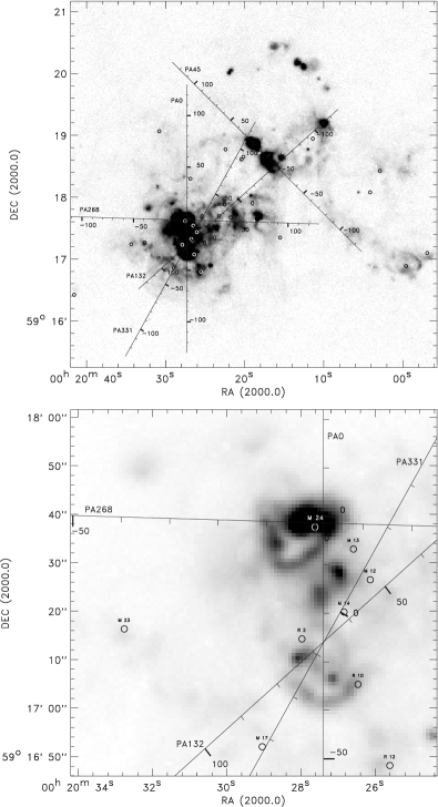
Figure 1: Positions of our five long slits on the H$\alpha$ image of IC 10: (a) the entire galaxy and (b) the bright region of current star formation. The long-slit spectrograms are marked up in arcsec. The circles designate the spectroscopically confirmed WR stars from Royer et al. (2001) and Massey and Holmes (2002).

Figure 2: Distributions of the line flux ratios $I([\textrm{OII}]\lambda 3727+3729\textrm{\AA})/I([\textrm{OIII}]\lambda 5007\textrm{\AA})$, $I([\textrm{SII}]\lambda 6717+6731\textrm{\AA})/I(\textrm{H}\alpha)$, $I([\textrm{NII}]\lambda 6583\textrm{\AA})/I(\textrm{H}\alpha)$, and $I([\textrm{OIII}]\lambda 5007\textrm{\AA})/I(\textrm{H}\beta)$ along slit PA132. Positions along the slits are given in arcsec at the horizontal axis in the lower panel. The numbers at the top of the lower panel denote the HII regions from the catalog by Hodge and Lee (1990). ”M10” marks the faint region around the WR star M10, and ”SS” designates the synchrotron superbubble.

Figure 3: Diagnostic diagrams of the line flux ratios: $I([\textrm{OIII}]\lambda 5007\textrm{\AA})/I(\textrm{H}\beta)$ versus $I([\textrm{SII}]\lambda 6717+6731\textrm{\AA})/I(\textrm{H}\alpha)$, versus $I([\textrm{NII}]\lambda 6583\textrm{\AA})/I(\textrm{H}\alpha)$, versus $I([\textrm{OII}]\lambda 3727+3729\textrm{\AA})/I([\textrm{OIII}]\lambda 5007\textrm{\AA})$, and versus $I([\textrm{NII}]\lambda 6583\textrm{\AA})/I([\textrm{SII}]\lambda 6717+6731\textrm{\AA}).$ The different symbols indicated at the bottom give the relative intensities averaged over individual HII regions from the catalog by Hodge and Lee (1990), over the region around WR M10, and over the synchrotron superbubble (SS). The uncertainties that exceed 0.1 dex are shown as the error bars.

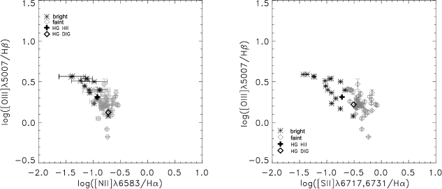
Figure 4: Diagnostic diagrams with bright ($F_{\textrm{H}\alpha}\geq 1.0\cdot 10^{-15}$ erg s^-1 cm^-2, black asterisks) and faint ($F_{\textrm{H}\alpha}\leq 1.0\cdot 10^{-15}$ erg s^-1 cm^-2, gray diamonds) regions. The measurements in 5-pixel ($1^{\prime\prime}.8$) fields along the slits PA0, PA132, and PA268 are presented. The heavy cross and diamond mark the galaxy-averaged values found by Hidalgo-Gamez (2005) for bright HII regions and the diffuse ionized gas (DIG).

Figure 5: Distributions of abundances $12+\log(\textrm{O/H})$ (a), $\log(\textrm{N}^{+}/\textrm{O})$ (b), and $\log(\textrm{S}^{+}/\textrm{O})$ (c) along our five slits. The HII region identifications are signed at the horizontal axis of the figures. The oxygen abundances $12+\log(\textrm{O/H})$ found using the methods by Izotov et al. (2006), Pilyugin and Thuan (2005), and Charlot and Longhetti (2001) are shown by dots with the solid, dotted, and dashed error bars, respectively.

Figure 5: (Contd.)

Figure 5: (Contd.)

Results of the spectra reduction are presented in Fig. 2 and Table 3. Fig. 2 shows the distributions of the relative line intensities $I$([OII]$\lambda 3727+3729$Å) / $I$([OIII]$\lambda 5007$Å), $I$([SII]$\lambda 6717+6731$Å) / $I$(H$\alpha$), $I$([NII]$\lambda 6583$Å) / $I$(H$\alpha$), and $I$([OIII]$\lambda$5007Å) / $I$(H$\beta$) along slit PA132. The slit is marked up in arcsec along the horizontal axis in the lower panel, the numbers at the top denote the HII regions from the catalog by Hodge and Lee (1990). ”M10” designates the faint region around the WR star M10 unrecorded in the catalog; SS designates the synchrotron superbubble. As it is seen in Fig. 1, the slit PA331 (positions 4–11) passes over the faint region near the HL111a in the southeast and positions 108–115 correspond to the northern periphery of the region HL50. To avoid overloading the figures and tables, these two regions on slit PA331 are designated in Tables 3 and 4 and all figures simply as HL111a and HL50, respectively. The slit PA268 (positions 68–71) passes between the bright nebulae HL46 and HL48; this region is designated below as HL46_48.

The columns in Table 3 show the designation of HII regions from the catalog by Hodge and Lee (1990), our long-slit spectrogram utilized for the estimations and the used positions on it, the relative intensities of the above-mentioned emission lines, and the [SII]$\lambda 6717/6731$ Å doublet line intensity ratios.

The interstellar extinction in Table 3 and Fig. 2 was taken into account. We determined the color excess $E(B-V)$ individually for each HII region, where possible. The most reliable results were obtained from the low-spectral-resolution spectrograms PA45 and PA331. For these spectrograms, we made our estimates by comparing the observed H$\alpha$:H$\beta$:H$\gamma$ flux ratio with the theoretical one: H$\alpha$:H$\beta$:$H\gamma=2.86:1.00:0.47$, which, according to Aller (1984), is valid for a typical electron density in a star-forming region of 30–300 cm^-3 when the electron temperature is accepted to be 11000 K (see discussion below). For the regions that did not fall in these slits, we assumed either the mean value of $E(B-V)$ = 0.95 mag or the color excess for the close region that fell into the slits PA 45 or PA 331. Our estimates of $E(B-V)$ for different regions in IC 10 range between 0.8 and 1.1 mag.

Diagnostic Diagrams of Relative Line Intensities

Fig. 3 shows the diagnostic diagrams of relative line intensities for IC 10 that are traditionally used to compare observations with computed ionization models: $I([\textrm{OIII}]\lambda 5007$Å) / $I(\textrm{H}\beta)$ versus $I$([SII]$\lambda 6717+6731$Å) / $I(\textrm{H}\alpha)$, versus $I$([NII]$\lambda 6583$Å) / $I(\textrm{H}\alpha)$, versus $I$([OII]$\lambda 3727+3729$Å) / $I([\textrm{OIII}]\lambda 5007\textrm{\AA})$, and versus $I$([NII]$\lambda 6583$Å) / $I([\textrm{SII}]\lambda 6717+6731\textrm{\AA})$. Different symbols indicate the relative intensities averaged over individual HII regions from the catalog by Hodge and Lee (1990), over the region around WR M10, and over the synchrotron superbubble (SS). The observing uncertainties greater than 0.1 dex are shown as the error bars in Fig. 3.

In Figs. 4a and 4b, the data were combined separately by bright ($F_{\textrm{H}\alpha}\geq 1.0\times 10^{-15}$ erg s^-1 cm^-2) and faint ($F_{\textrm{H}\alpha}\leq 1.0\times 10^{-15}$ erg s^-1 cm^-2) emission regions. The measurements along the 1.8” wide slits PA0, PA132, and PA268 are shown in Fig. 4. The crosses and diamonds in these figures also indicate the galaxy-averaged values found by Hidalgo-Gamez (2005) for bright HII regions and faint regions of diffuse ionized gas (DIG) (see the “Discussion” section).

Estimates of the Relative Oxygen, Nitrogen, and Sulfur Abundances

The spectra enable us to estimate the relative oxygen abundance in a large number of galactic HII regions, both bright and faint. Previously, such estimates were made for only three brightest regions: HL111, HL45, and the compact clump HL106a inside HL106 (Lequeux et al. 1979; Garnett 1990; Richer et al. 2001; Lee et al. 2003).

Table 2: Emission line flux ratios at the points of intersection of our slit spectrograms

Spectrogram	$\log$($I([\textrm{OIII}]\lambda 5007~{}\textrm{\AA})/I(\textrm{H}\beta)$)	$\log$($I([\textrm{SII}]\lambda 6717+6731~{}\textrm{\AA})/I(\textrm{H}\alpha)$)
	1. Intersection of PA0, PA132, PA331
PA0	$0.32\pm 0.03$	$-0.86\pm 0.02$
PA132	$0.30\pm 0.03$	$-0.68\pm 0.04$
PA331	$0.31\pm 0.03$	$-0.84\pm 0.03$
	2. Intersection of PA0, PA268
PA0	$0.55\pm 0.03$	$-1.10\pm 0.04$
PA268	$0.55\pm 0.02$	$-1.25\pm 0.03$
	3. Intersection of PA268, PA331
PA268	$0.22\pm 0.04$	$-0.45\pm 0.03$
PA331	$0.18\pm 0.05$	$-0.47\pm 0.04$
	4. Intersection PA132, PA268
PA132	$0.02\pm 0.04$	$-0.18\pm 0.08$
PA268	$0.13\pm 0.05$	$-0.33\pm 0.04$
	5. Intersection of PA45, PA331
PA45	$0.44\pm 0.11$	$-0.79\pm 0.04$
PA331	$0.48\pm 0.04$	$-0.85\pm 0.03$
	6. Intersection of PA45, PA132
PA45	$0.61\pm 0.21$	$-1.06\pm 0.11$
PA132	$0.48\pm 0.07$	$-0.81\pm 0.23$

Table 3: Emission line flux ratios

Region	Slit/position	$\frac{I([\textrm{OIII}]5007)}{I(\textrm{H}\beta)}$	$\frac{I([\textrm{SII}]6717+6731)}{I(\textrm{H}\alpha)}$	$\frac{I([\textrm{NII}]6583)}{I(\textrm{H}\alpha)}$	$\frac{I([\textrm{SII}]6717}{I([\textrm{SII}]6731}$	$\frac{I([\textrm{OII}]3727+3729)}{I([\textrm{OIII}]5007)}$
HL111a	PA0 [$-13$, $-9$]	$1.90\pm 0.03$	$0.178\pm 0.002$	$0.134\pm 0.003$	$1.39\pm 0.03$	$2.64\pm 0.33$
	PA331 [4, 11]	$2.09\pm 0.12$	$0.201\pm 0.003$	$0.099\pm 0.003$	$1.10\pm 0.01$	$1.44\pm 0.22$
HL111b	PA0 [$-20$, $-15$]	$1.51\pm 0.05$	$0.183\pm 0.03$	$0.148\pm 0.003$	$1.47\pm 0.05$	$3.63\pm 0.41$
HL111c	PA0 [$-4$, $3$]	$3.52\pm 0.02$	$0.081\pm 0.001$	$0.069\pm 0.001$	$1.41\pm 0.03$	$0.80\pm 0.10$
	PA268 [$-6$, $5$]	$3.47\pm 0.01$	$0.063\pm 0.001$	$0.047\pm 0.001$	$1.40\pm 0.01$	$0.50\pm 0.02$
HL111d	PA268 [$-12$, $-8$]	$2.95\pm 0.01$	$0.137\pm 0.001$	$0.097\pm 0.001$	$1.41\pm 0.02$	$1.16\pm 0.08$
HL111e	PA0 [$-7$, $-5$]	$2.44\pm 0.06$	$0.138\pm 0.002$	$0.101\pm 0.002$	$1.50\pm 0.05$	$1.62\pm 0.41$
HL106	PA0 [$-42$, $-21$]	$2.89\pm 0.07$	$0.161\pm 0.004$	$0.117\pm 0.004$	$1.46\pm 0.08$	$1.40\pm 0.41$
	PA132 [62, 80]	$2.31\pm 0.03$	$0.191\pm 0.007$	$0.102\pm 0.006$	$1.26\pm 0.09$	$1.23\pm 0.08$
	PA331 [$-20$, $-8$]	$2.42\pm 0.11$	$0.144\pm 0.002$	$0.066\pm 0.02$	$1.02\pm 0.01$	$1.11\pm 0.41$
SS	PA0 [$-60$, $-55$]	$0.75\pm 0.10$	$0.713\pm 0.017$	$0.247\pm 0.013$	$1.58\pm 0.08$	$4.24\pm 0.44$
	PA132 [84, 100]	$1.33\pm 0.13$	$0.745\pm 0.100$	$0.230\pm 0.056$	$1.24\pm 0.26$	$3.49\pm 0.42$
	PA331 [$-40$, $-27$]	$1.87\pm 0.10$	$0.625\pm 0.006$	$0.207\pm 0.04$	$1.63\pm 0.09$	$1.99\pm 0.43$
HL37	PA45 [$-12$, $-6$]	$3.34\pm 0.24$	$0.073\pm 0.002$	$0.033\pm 0.012$	$1.55\pm 0.05$	$0.87\pm 0.26$
	PA132 [$-52$, $-44$]	$2.85\pm 0.05$	$0.180\pm 0.030$	$0.064\pm 0.024$	$0.99\pm 0.22$	$0.89\pm 0.13$
HL45	PA45 [$-4$, $3$]	$4.86\pm 0.09$	$0.079\pm 0.005$	$0.045\pm 0.002$	$1.12\pm 0.03$	$0.22\pm 0.05$
HL50	PA45 [12, 27]	$3.44\pm 0.08$	$0.073\pm 0.005$	$0.045\pm 0.002$	$1.35\pm 0.05$	$0.69\pm 0.14$
	PA331 [108, 115]	$3.05\pm 0.08$	$0.162\pm 0.009$	$0.086\pm 0.002$	$1.49\pm 0.14$	$1.11\pm 0.10$
HL100	PA132 [49, 58]	$1.65\pm 0.02$	$0.364\pm 0.020$	$0.179\pm 0.023$	$1.24\pm 0.11$	$2.69\pm 0.23$
HL89	PA132 [35, 43]	$1.32\pm 0.2$	$0.446\pm 0.029$	$0.168\pm 0.039$	$1.19\pm 0.12$	$4.39\pm 0.32$
M10	PA132 [20, 30]	$1.49\pm 0.06$	$0.753\pm 0.065$	$0.165\pm 0.026$	$1.03\pm 0.13$	$6.41\pm 0.53$
HL67	PA132 [5, 15]	$1.61\pm 0.06$	$0.578\pm 0.076$	$0.142\pm 0.044$	$0.89\pm 0.15$	$4.13\pm 0.48$
HL41	PA132 [$-43$, $-39$]	$1.58\pm 0.05$	$0.254\pm 0.011$	$0.126\pm 0.013$	$1.07\pm 0.09$	$0.43\pm 0.41$
HL36	PA132 [$-61$, $-55$]	$2.86\pm 0.03$	$0.137\pm 0.019$	$0.065\pm 0.007$	$0.94\pm 0.22$	$0.60\pm 0.17$
HL22	PA132 [$-116$, $-108$]	$1.53\pm 0.03$	$0.158\pm 0.011$	$0.126\pm 0.007$	$1.17\pm 0.13$	$2.60\pm 0.37$
HL46_48	PA268 [68, 71]	$1.49\pm 0.08$	$0.320\pm 0.011$	$0.200\pm 0.010$	$1.66\pm 0.09$	$2.94\pm 0.43$

Table 4: Relative O, N⁺, and S⁺ abundances

Region	Slit/position	$12+\log(\textrm{O/H})$ (1)	$12+\log(\textrm{O/H})$ (2)	$12+\log(\textrm{N}^{+}/\textrm{H})$	$12+\log(\textrm{S}^{+}/\textrm{H})$
HL111a	PA0 [$-13$, $-9$]	$8.34\pm 0.24$	$8.28\pm 0.12$	$6.26\pm 0.13$	$5.46\pm 0.12$
	PA331 [4, 11]	$8.05\pm 0.34$	$8.15\pm 0.15$	$6.54\pm 0.16$	$6.00\pm 0.16$
HL111b	PA0 [$-20$, $-15$]	$8.27\pm 0.22$	$8.29\pm 0.13$	$6.38\pm 0.13$	$5.55\pm 0.13$
HL111c	PA0 [$-4$, $3$]	$8.24\pm 0.15$	$8.24\pm 0.10$	$5.92\pm 0.10$	$5.07\pm 0.10$
	PA268 [$-6$, $5$]	$7.94\pm 0.10$	$8.15\pm 0.10$	$6.05\pm 0.12$	$6.56\pm 0.22$
HL111d	PA268 [$-12$, $-8$]	$8.28\pm 0.11$	$8.05\pm 0.16$	$6.10\pm 0.18$	$5.33\pm 0.19$
HL111e	PA0 [4–7, $-5$]	$8.29\pm 0.38$	$8.24\pm 0.18$	$6.21\pm 0.19$	$5.42\pm 0.18$
HL106	PA0 [$-42$, $-21$]	$8.41\pm 0.42$	$8.28\pm 0.22$	$6.21\pm 0.22$	$5.41\pm 0.22$
	PA132 [62, 80]	$8.06\pm 0.14$	$8.15\pm 0.10$	$6.01\pm 0.10$	$5.32\pm 0.10$
	PA331 [$-20$, $-8$]	$8.03\pm 0.42$	$8.14\pm 0.27$	$6.39\pm 0.27$	$5.88\pm 0.28$
SS	PA0 [$-60$, $-55$]	$7.59\pm 0.42$	$8.04\pm 0.43$	$6.44\pm 0.41$	$5.97\pm 0.43$
	PA132 [84, 100]	$8.07\pm 0.18$	$8.22\pm 0.21$	$6.45\pm 0.38$	$6.00\pm 0.41$
	PA331 [$-40$, $-27$]	$8.12\pm 0.42$	$8.19\pm 0.39$	$6.88\pm 0.39$	$6.50\pm 0.39$
HL37	PA45 [$-12$, $-6$]	$8.23\pm 0.42$	$8.23\pm 0.20$	$6.23\pm 0.24$	$5.63\pm 0.21$
	PA132 [$-52$, $-44$]	$8.07\pm 0.23$	$8.17\pm 0.10$	$5.96\pm 0.22$	$5.39\pm 0.17$
HL45	PA45 [$-4$, $3$]	$7.92\pm 0.17$	$8.21\pm 0.10$	$6.24\pm 0.12$	$5.60\pm 0.10$
HL50	PA45 [12, 27]	$8.10\pm 0.36$	$8.20\pm 0.13$	$6.32\pm 0.14$	$5.58\pm 0.13$
	PA331 [108, 115]	$8.30\pm 0.16$	$8.25\pm 0.10$	$6.56\pm 0.10$	$5.80\pm 0.10$
HL100	PA132 [49, 58]	$8.16\pm 0.16$	$8.23\pm 0.10$	$6.31\pm 0.15$	$5.65\pm 0.10$
HL89	PA132 [35, 43]	$8.23\pm 0.13$	$8.29\pm 0.10$	$6.30\pm 0.27$	$5.72\pm 0.10$
M10	PA132 [20, 30]	$8.74\pm 0.36$	$8.49\pm 0.19$	$6.43\pm 0.29$	$6.04\pm 0.20$
HL67	PA132 [5, 15]	$8.52\pm 0.23$	$8.36\pm 0.13$	$6.34\pm 0.20$	$5.86\pm 0.17$
HL41	PA132 [$-43$, $-39$]	$7.73\pm 0.42$	$7.79\pm 0.39$	$6.24\pm 0.39$	$5.55\pm 0.39$
HL36	PA132 [$-61$, $-55$]	$7.86\pm 0.42$	$8.09\pm 0.15$	$5.96\pm 0.19$	$5.28\pm 0.19$
HL22	PA132 [$-116$, $-108$]	$8.28\pm 0.12$	$8.18\pm 0.14$	$6.25\pm 0.16$	$5.44\pm 0.16$
HL46_48	PA268 [68, 71]	$8.10\pm 0.40$	$8.21\pm 0.21$	$6.58\pm 0.23$	$5.85\pm 0.21$
from observations by Lequeux et al. (1979)
HL111		7.74	8.17	6.23	5.48
HL45		7.92	8.31	6.24	5.40

For the abundance analysis, we employ equation (24) from Pilyugin and Thuan (2005), which is the revisited calibration dependence of the oxygen abundance $12+\log(\textrm{O/H})$ on the flux ratios of strongest [OII] and [OIII] lines. The classical method of estimation from the so-called oxygen abundance indicator $R_{23}$ suggested by Pagel et al. (1979) and widely used previously was modified in a series of papers by Pilyugin (see Pilyugin and Thuan (2005)) and is based on two parameters: $R_{23}$ and the excitation parameter $P$. For verification purposes, we also incorporate other techniques for the abundance estimation developed by Izotov et al.(2006) and by Charlot and Longhetti (2001).

The distributions of abundances $12+\log(\textrm{O/H})$ along the five long slits obtained are shown in Fig. 5a and presented in Table 4. The mean oxygen abundances in the bright HII regions are shown by dots with the error bars.

As was noted by Pilyugin and Thuan (2005) their (24) relation is most reliable for $P$ in the range from $\simeq 0.55$ to $\simeq 1$. Having eliminated the points corresponding to $P<0.55$, we verified that this did not change significantly our averaged estimates of the oxygen abundance but only slightly increased the measurement accuracy.

To estimate the relative nitrogen and sulfur abundances in various HII regions, we used Eqs. (6) and (8) from Izotov et al. (2006)

The resulting sulfur and nitrogen abundances in our regions of IC 10 are shown in Fig.5a and 5b, respectively. Note that we actually estimate the S⁺ abundance, because we disregarded the S²⁺ emission in the $[\textrm{SIII}]\lambda 6312$ line that we can measure only in HL111c. This is also true for the nitrogen abundance.

To properly estimate the N/O and S/O ratios, we also found the relative oxygen abundance $12+\log(\textrm{O/H})$ using Eqs. (3) and (5) from Izotov et al. (2006)

The characteristic electron density in galactic ionized-gas regions that we found from the [SII] line flux ratio varies within the range from 30 to 300–400 cm^-3 and these variations have virtually no effect on the abundance estimates.

We assume the electron temperature to be $T_{e}(\textrm{OIII})=11000$ K in all HII regions. There are three reasons for choosing this value. First, it is close to a temperature of about 11600 K that we determined from the oxygen line flux ratio in HL111c. This is the only bright HII region where we can detect the [OIII]$\lambda 4363$ Å auroral line. Unfortunately, the line flux has a large uncertainty, because the line is weak. Second, the adopted value lies between the ones obtained by Lequeux et al. (2003) and Lee et al. (2003) for the three brightest HII regions in the galaxy. Third, this electron temperature provides the best agreement between the oxygen abundances derived according to Pilyugin and Thuan (2005), and Izotov et al.(2006) The temperature in the [OII] emission region was found from the relation (Izotov et al. 2006)

$$t(\textrm{OII})=-0.744+t(\textrm{OIII})\cdot(2.338-0.610t(\textrm{OIII})).$$

We assume the same temperature for the [SII] and [NII] emission region.

The obtained results are collected in Table 4. Its columns show the designation of the HII region according to the catalog by Hodge and Lee (1990), the spectrogram used for our estimates and the positions on it, and the derived mean oxygen, nitrogen, and sulfur abundances. The oxygen abundances estimated using Eq. (24) from Pilyugin and Thuan (2005) are denoted in Table 4 by (1). Those estimated with Eqs. (3) and (5) from Izotov et al. (2006) are denoted by (2).

We did not average the abundances found from different spectra for the same HII region, since they correspond to different slit positions on the nebula and could differ due to different physical conditions: the density and porosity of interstellar medium, loci of the radiation sources, etc.

The lower rows in Table 4 show the abundances in two regions: HL 111 and HL 45 which correspond to the regions 1 and 2, from Fig. 1 by Lequeux et al. (1979). We derived the abundances for the relative line intensities measured by Lequeux et al. (1979). In both cases the slit in this paper was in the east–west direction. The region over which the relative abundances were averaged spans 3”.8 $\times$ 12”.4. Since no localization of the spectrograms is given by Lequeux et al.(1979), we can make the comparison only approximately.

DISCUSSION

Interstellar Extinction

Variations of the color excess that we revealed here for different galactic regions lie within the range 0.8 - 1.1 mag. This is considerably smaller than the difference from literature, where it ranges from $E(B-V)$ = 0.47 mag to $E(B-V)$ = 2.0 mag (see Sakai et al. 1999; Demers et al. 2004; and references therein). In the three brightest HII regions, Lee et al. (2003) found $E(B-V)$ = 0.79 – 1.2 mag, which is similar to our estimates. Variations of $E(B-V)$ that we observed can be naturally explained by two factors. First, a local higher extinction is possible, since the brightest star-forming region is projected to the densest cloud of neutral hydrogen and molecular gas in the galaxy, and hence can be partly embedded into it. A similar effect was also observed by other authors. In particular, the extinction estimated by Borissova et al. (2000) from the flux ratio of the Br$\gamma$ and H$\alpha$ lines in the two brightest nebulae HL111 and HL45 is considerably higher than that found from stars. Second, a local lower extinction is possible if the stellar wind and SN explosions in young groups sweep out the surrounding dense gas. In particular, in the central star-forming region Vacca et al. (2007) found $E(B-V)$ = 0.6 mag from massive blue stars and concluded that the young stars born in the last star formation episode are located at the front boundary of the above-mentioned dense cloud in front of the old stellar population.

In this paper we present one of the most detailed studies of the oxygen, nitrogen, and sulfur abundances in IC 10. Previously, Lequeux et al. (1979) found $12+\log(\textrm{O/H})=8.17$ for HL111 and $12+\log(\textrm{O/H})=8.45$ for HL45. The lower rows in Table 4 give our estimates based on the measurements by Lequeux et al. (1979). According to Garnett (1990), $12+\log(\textrm{O/H})=8.19$ for HL45. According to Richer et al. (2001), $12+\lg(\textrm{O/H})=8.23\pm 0.09$ in the brightest nebula HL111c. For the brightest objects with detected [OIII]$\lambda 4363$ Å line, Lee et al. (2003) found that $12+\log(\textrm{O/H})=8.32\pm 0.14$ in HL111c, $8.05\pm 0.18$ in HL111e, $12+\log(\textrm{O/H})\geq 7.96$ in HL111b, and $12+\log(\textrm{O/H})\geq 7.60$ in the clump HL106a inside HL106. In the latter two objects, only the upper abundance limit was estimated. As we see, all listed results are in a good agreement with our observations of HII regions in IC 10.

As our measurements showed, the relative oxygen line intensities and, accordingly, the relative oxygen abundances vary in a wide range, from 7.6 to 8.5. To understand whether it is related to the observational errors or to the actual differences between HII regions, we presented the relative intensities found, respectively, for bright and faint objects in Figs. 4a and 4b. As follows from the figure, the measurement errors are slightly larger for the faint regions than that in the bright ones. However, the scatter of values in the faint regions does not exceed significantly that for the bright ones. Therefore, we conclude that the oxygen abundance variations in the galaxy are most likely real. At the same time, the systematic difference between the relative intensities in the bright and faint regions is observed (see below).

The relative oxygen abundance averaged over all galactic regions that we investigated here is $12+\log(\textrm{O/H})=8.17\pm 0.35$, which corresponds to the metallicity $Z=0.18\pm 0.14Z_{\odot}$.

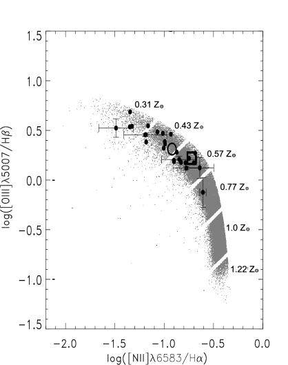
Figure 6: Comparison of our line intensity ratios with results by Cid Fernandes et al. (2007) and Asari et al. (2007). The mean metallicity in each of the gray sectors is shown to the right of the localization band of 85000 starburst galaxies. The circle and the square indicate the galaxy-averaged values found by Hidalgo-Gamez (2005) for bright HII regions and the diffuse ionized gas (DIG), respectively.

Diagnostic Diagrams of Relative Line Intensities

The relative intensities of diagnostic lines in the bright nebulae and faint regions of diffuse ionized gas (DIG) in the whole galaxy and over its four fields taken apart were estimated previously by Hidalgo-Gamez (2005) from nine spectrograms combined into one wide band. According to this paper, the galaxy-averaged relative intensities are $I([OIII]5007\textrm{\AA})/I(\textrm{H}\beta)=1.86$, $I$($[\textrm{NII}]\lambda 6583$Å) / $I(\textrm{H}\alpha)=0.16$, and $I$($[\textrm{SII}]\lambda 6717$Å) / $I$($\textrm{H}\alpha)=0.28$. The values averaged over the bright nebulae are $I$($[\textrm{OIII}]\lambda 5007$Å) / $I(\textrm{H}\beta)=2.05$, $I$($[\textrm{NII}]\lambda 6583$Å) / $I(\textrm{H}\alpha)=0.12$, $I$($[\textrm{SII}]\lambda 6717$Å) / $I(\textrm{H}\alpha)=0.19$. The values averaged over the faint diffuse ionized gas (DIG) are $I$($[\textrm{OIII}]\lambda 5007$Å) / $I(\textrm{H}\beta)=1.66$, $I$($[\textrm{NII}]\lambda 6583$Å) / $I(\textrm{H}\alpha)=0.19$, $I$($[\textrm{SII}]\lambda 6717$Å) / $I(\textrm{H}\alpha)=0.31$. Our measurements of these line ratios in individual HII regions are in good agreement with the values above, given the observational errors.

As follows from Figs. 4a and 4b, similar to other Irr galaxies investigated in detail, the diagnostic diagrams slightly differ between the bright and faint regions of IC 10: the relative intensities of [SII] lines are appreciably higher in faint regions as well as those of [NII] lines are also slightly higher, whereas $I$([OIII]$\lambda 5007$ Å)/$I$(H_β) weakens in these regions. The similar picture is also observed in spiral galaxies, for example, in M31 (see Galarza et al. 1999). The value of $I$([SII])/$I$(H$\alpha$) in the bright compact HII regions is lower than that in the faint diffuse and ring nebulae, not to mention the DIG. The noted differences can be explained by a decrease in the ionization parameter when transiting from the compact to faint diffuse regions. This effect is predicted by photoionization models. The contribution from the gas emission behind the front of the shocks triggered by supernova explosions and stellar wind also leads to the same effect of the relative intensity $I$([SII])/$I$(H$\alpha$) enhancement. The filamentary structure of the entire H$\alpha$ emission region in the galaxy suggests that the shocks play a prominent role in IC 10.

It should be noted that the constructed diagnostic lines diagrams agree poorly with the currently available photoionization models for the metallicity $Z=0.2Z_{\odot}$ found above from strong oxygen lines. In particular, the observed diagnostic diagrams are consistent with the families of theoretical diagnostic curves (Dopita et al. 2006) only for a metallicity from $Z=0.4Z_{\odot}$ to $Z$= (1 - 2) $Z_{\odot}$.

In Fig. 6, our data are compared with the results of Cid Fernandes et al. (2007) and Asari et al. (2007), who summarized the gas metallicity estimates for $\simeq 85000$ starburst galaxies. On the $I([\textrm{OIII}]\lambda 5007\textrm{\AA})/I(H\beta)$ versus $I([\textrm{NII}]\lambda 6583\textrm{\AA})/I(\textrm{H}\alpha)$ diagram, these authors give the number of objects in each sector of the galaxy localization band and the mean metallicity that corresponds to the sector. As we see, the HII regions in IC 10 fall nicely on the galaxy localization band but fall within the range of metallicities from $Z=0.3Z_{\odot}$ to $Z=0.6Z_{\odot}$. One distinctive region in IC 10, the synchrotron superbubble, falls near $Z=0.8Z_{\odot}$. This object is discussed below. Note, however, that Asari et al. (2007) recorded a systematic shift by 0.2 dex between their metallicity estimates and those of Pilyugin and Thuan (2005) and Izotov et al. (2006) for 177 “common” objects made from the relations that we used here. It turns out that the lower the metallicity, the larger the shift. For this reason, Asari et al. adopted the metallicity $Z=0.2Z_{\odot}$ for Sector A rather than $Z=0.3Z_{\odot}$ and therefore $Z=0.2Z_{\odot}$ is the lower boundary of the range into which our regions of IC 10 fall.

It is also interesting to compare the observed diagnostic diagrams with the theoretical photoionization models by Charlot and Longhetti (2001), since these authors separately took into account the changes in each of the parameters defining the model calculations, such as the cluster age, the initial mass function (IMF), ionization parameter, density of interstellar medium, and metallicity.

Figure 7: Comparison of the line flux ratios on diagnostic diagrams with the model calculations by Charlot and Longhetti (2001). The large squares, circles, and triangles in the left panels (a) mark the regions of reduced ($Z=0.2Z_{\odot}$), solar ($Z=Z_{\odot}$), and enhanced ($Z=2Z_{\odot}$) metallicity, respectively, in accordance with the model calculations. The same symbols in the right panels (b) indicate the model calculations for the effective ionization parameters $\log U_{0}-3.0$, $-2.5$, and $-2.0$, respectively.

Comparison of the diagnostic diagrams for IC 10 with the distributions of ${I([\textrm{OIII}]/I(\textrm{H}\beta)}$ as a function of $I$([OII])/$I$([OIII]), $I$([SII])/$I$(H$\alpha$), and $I$([NII])/$I$([SII]) constructed by Charlot and Longhetti (2001) for galaxies of various types and HII regions showed an excellent agreement between them and our observing line flux ratios. In Fig. 7 our observations are compared with the models computed by Charlot and Longhetti (2001) for various metallicities and various effective ionization parameters. The large square, circle, and triangle on our diagnostic diagrams (left panels) mark the regions of reduced ($Z=0.2Z_{\odot}$), solar ($Z=Z_{\odot}$), and enhanced ($Z=2Z_{\odot}$) metallicity from models by Charlot and Longhetti (2001), see Figs. 1, 2, and 3 in their paper. The large square, circle, and triangle on the right panels indicate three values of the model flux ratios for the effective ionization parameter $\log U_{0}$ of $-3.0$, $-2.5$, and $-2.0$ from the calculations by Charlot and Longhetti (2001). As we see, in complete agreement with the model calculations, the $I([\textrm{OIII}]\lambda 5007\textrm{\AA})/I(\textrm{H}\beta)$ versus $I([\textrm{NII}]\lambda 6583\textrm{\AA})/I([\textrm{SII}]\lambda 6717+6731\textrm{\AA})$ diagnostic diagrams are most promising for estimating the metallicity of the galactic gaseous medium. Positions of our HII regions in IC 10 on the diagnostic diagrams correspond to the metallicities within the range of $Z$= (0.2 – 1) $Z_{\odot}$. The dependences of $I([\textrm{OIII}]\lambda 5007\textrm{\AA})/I(\textrm{H}\beta)$ on $I$([OII])/$I$([OIII]) and of $I([\textrm{OIII}]\lambda 5007\textrm{\AA})/I(\textrm{H}\beta)$ on $I([\textrm{SII}]\lambda 6717+\linebreak+6731\textrm{\AA})/I(\textrm{H}\alpha)$ are well explained by variations in the ionization parameter.

The differences between the metallicity of individual HII regions in the galaxy found from the $R_{23}$ parameter and the metallicity determined by comparing diagnostic diagrams with theoretical photoionization models can be explained by a number of factors. First of all, the photoionization models are computed for rich star clusters. In particular, Dopita et al. (2006) assumed a cluster mass of $M\geq 10^{3}M_{\odot}$, the IMF by Miller and Scalo ranges from 1 to $100M_{\odot}$, while the star clusters in IC 10 are comparatively poor (see Hunter 2001).

In addition, the contribution from the gas emission behind the front of the shocks can be significant in IC 10, as suggested by the filamentary structure of the entire star-forming region in this galaxy. Actually, the term “diffuse ionized gas” (DIG) can be applied to IC 10 only conditionally, because the faint emission regions are characterized mostly as filamentary shell and/or arc structure. Therefore, the faintest regions inside a number of shells that appear diffuse most likely represent the front or back sides of the shells.

The synchrotron superbubble in IC 10 is a unique object and deserves a more detailed discussion. According to Lozinskaya and Moiseev (2007) and Lozinskaya et al. (2008), the image in [SII] lines better than in H$\alpha$ reveals the optical shell identified with the synchrotron superbubble. The expansion velocity of the bright knots and filaments in the optical shell found in these papers, 50–80 km s^-1, confirms the estimate by Ramsey et al. (2006). The gas mass is $M\simeq 4\times 10^{5}M_{\odot}$ and the kinetic energy is $E_{\textrm{kin}}\simeq(1-3)\cdot 10^{52}$ erg. This amount of released energy corresponds to the explosions of ten supernovae plus the stellar wind from their host association. Alternatively, the superbubble may be a result of a hypernova explosion, as was suggested by Lozinskaya and Moiseev (2007). The kinematic age of the superbubble, $t\simeq$ (3 – 7)$\cdot 10^{5}$ yr, is a strong argument for a hypernova, because it takes more than $t\simeq 10^{7}$ yr for the explosions of ten supernovae in a local galactic region.

As it can be seen in Fig. 1, the regions from $85^{\prime\prime}$ to $120^{\prime\prime}$ on spectrogram PA132, from $-60^{\prime\prime}$ to $-25^{\prime\prime}$ on spectrogram PA331, and from $-50^{\prime\prime}$ to $-80^{\prime\prime}$ on spectrogram PA0 (the latter passes over the very edge of the superbubble) correspond to the synchrotron superbubble.

Our measurements indicate that the relative intensity $I([\textrm{SII}]\lambda 6717+6731\textrm{\AA})/I(\textrm{H}\alpha)$ in the region of the synchrotron superbubble reaches 0.7–0.75, which strongly suggests a gas emission behind the shock front (Dopita and Sutherland 1995, 1996). This is also suggested by the ratios of $I([\textrm{NII}]\lambda 6583\textrm{\AA})/I(\textrm{H}\alpha)\simeq 0.25$ and $I([\textrm{OII}]\lambda 3727+3729\textrm{\AA})/I([\textrm{OIII}]\lambda 5007\textrm{\AA})\simeq 2-4$ that are higher than those in the nearby bright region HL106, and also by the lower relative intensity $I([\textrm{OIII}]\lambda 5007\textrm{\AA})/I(\textrm{H}\beta)$.

The region of the synchrotron superbubble on the diagnostic diagrams also differs from HII regions by a lower ratio $I([\textrm{OIII}]\lambda 5007\textrm{\AA})/I(\textrm{H}\beta)$ and by high $I([\textrm{SII}]\lambda 6717+6731\textrm{\AA})/I(\textrm{H}\alpha)$,
$I([\textrm{NII}]\lambda 6583\textrm{\AA})/I(\textrm{H}\alpha)$, and $I([\textrm{OII}]\lambda 3727+3729\textrm{\AA})/I([\textrm{OIII}]\lambda 5007\textrm{\AA})$. This suggests the dominance of the collisional excitation and is typical in old supernova remnants.

Lozinskaya and Moiseev (2007) found a mean $n_{e}\simeq$ 20 – 30 cm^-3 from the intensities of the [SII]($\lambda 6717/6731$Å) lines for the brighter northern part of the superbubble (the region 90^′′ – 105^′′ on PA132), where the errors are relatively small. For the region $-50^{\prime\prime}$ – $-60^{\prime\prime}$ on spectrogram PA0, we find a similar mean density $n_{e}\simeq$ 30 – 40 cm^-3. In the southern faint part of the superbubble, individual knots can be distinguished in the spectrogram PA132 in which the density reaches $n_{e}\simeq$ 200 – 300 cm^-3, but the accuracy of these estimates is low. The gas density northward of the synchrotron superbubble (the positions range between $80^{\prime\prime}$ – 90^′′ on PA132) is $n_{e}\simeq 200$ cm^-3.

The oxygen abundance estimate in the region of the synchrotron superbubble is ambiguous. In general, the present-day models of the gas emission spectrum behind the shock front developed by Allen et al. (2008) allow the abundances of heavy elements, in particular oxygen, to be determined from the available diagnostic relative line intensities if the ambient gas density and the shock velocity are known. However, in our case the problem is complicated by the presence of the WR star M17 in the central region of the synchrotron superbubble, whose ionizing radiation may be significant or even dominant in close neighborhoods. On the other hand, we cannot properly use the technique applied above to HII regions without taking into account the gas emission behind the shock front.

A careful calculation including both emission mechanisms is beyond the scope of this paper. Below we formally estimate the oxygen abundance in the synchrotron superbubble independently by two methods, realizing that both are improper. Employing the $R_{23}$ parameter, we found the abundances $12+\log(\textrm{O/H})=8.07\pm 0.18$ from spectrogram PA132, $7.59\pm 0.42$ from PA0, and $8.12\pm 0.42$ from PA331 using the technique of Pilyugin and Thuan (2005) or, respectively, $8.22\pm 0.21$ from spectrogram PA132, $8.04\pm 0.43$ from PA0, and $8.19\pm 0.39$ from PA331 using the technique of Izotov et al. (2006) (see Table 4). Since the measurements were made for three different regions of a very faint extended object, these independent estimates of the oxygen abundance are in a very good agreement.

A detailed kinematic study of the synchrotron superbubble (Lozinskaya et al. 2008) clearly revealed weak H$\alpha$ wings in the velocity range from $-200$ to $-450$ km s^-1. These high-velocity features in the line correspond to the velocity of the shock wave triggered by a hypernova explosion of about 100–200 km s^-1. Comparison with the models of gas emission behind the front of a shock (Allen et al. 2008) propagating with such velocity gives the best agreement at the abundance $12+\log(\textrm{O/H})\simeq 8.15$ with the models of purely collisional excitation, or $12+\log(\textrm{O/H})\simeq 8.35$ with the models that include the gas pre-ionization by a shock.

CONCLUSIONS

We present the most detailed to-date study of the O, N⁺, and S⁺ abundances of the individual HII regions and the synchrotron superbubble in the dwarf Irr galaxy IC 10 that we estimated from five spectrograms taken with the SCORPIO instrument at the 6-m SAO telescope.

The relative O, N⁺, and S⁺ abundances in individual HII regions of the galaxy IC 10 lie within the following ranges: $12+\log(\textrm{O/H})$ = 7.59 – 8.52 , $12+\log(\textrm{N}^{+}/\textrm{H})$ = 5.92 – 6.58 , and $12+\log(\textrm{S}^{+}/\textrm{H})$ = 5.00 – 6.00. The mean metallicity of the galaxy’s gaseous medium is $Z=0.18\pm 0.14Z_{\odot}$. The metallicity estimates from the comparison of diagnostic diagrams with photoionization models are found to be less reliable than those from the strong oxygen line ratios.

The oxygen abundance estimates in the synchrotron superbubble from the measured relative line intensities must be based on the model of the combined action of a shock (the result of a hypernova explosion) and ionizing radiation (the presence of a WR star in the central region). So far the estimates have been made separately within the framework of these two models. With the model of an HII region, we found that $12+\log(\textrm{O/H})=$7.59 – 8.34. The comparison with the models of gas emission behind the front of a shock propagating with the velocity of 100–200 km s^-1 gives the best agreement at the abundance $12+\log(\textrm{O/H})\simeq 8.15$ with the models of purely collisional excitation or $12+\log(\textrm{O/H})\simeq 8.35$ for the models that include the gas pre-ionization by a shock.

REFERENCES

V. L. Afanasiev and A. V. Moiseev, Pis’ma Astron. Zh. 31, 269 (2005) [Astron. Lett. 31, 194 (2005)].
M. G. Allen, B. A. Groves, M. A. Dopita, et al., Astrophys. J. Suppl. Ser. 178, 20 (2008).
L. H. Aller, Physics of Thermal Gaseous Nebulae (Reidel, Dordrecht, 1984).
N. V. Asari, R. Cid Fernandes, G. Stasinska, et al., Mon. Not. R. Astron. Soc. 381, 263 (2007).
J. Borissova, L. Georgiev, M. Rosado, et al., Astron. Astrophys. 363, 130 (2000).
A. Bullejos and M. Rozado, Rev. Mex. Astron. Astrophys. 12, 254 (2002).
S. Charlot and M. Longhetti, Mon. Not. R. Astron. Soc. 323, 887 (2001).
K. T. Chyzy, J. Knapik, D. J. Bomans, et al., Astron. Astrophys. 405, 513 (2003).
R. Cid Fernandes, N. V. Asari, L. Sodre, et al., Mon. Not. R. Astron. Soc. 375, 16 (2007).
P. A. Crowther, L. Drissen, J. B. Abbott, et al., Astron. Astrophys. 404, 483 (2003).
S. Demers, P. Battinelli, and B. Letarte, Astron. Astrophys. 424, 125 (2004).
M. A. Dopita and R. S. Sutherland, Astrophys. J. 455, 468 (1995).
M. A. Dopita and R. S. Sutherland, Astrophys. J. Suppl. Ser. 102, 161 (1996).
M. A. Dopita, J. Fischera, R. S. Sutherland, et al., Astrophys. J. Suppl. Ser. 167, 177 (2006).
V. C. Galarza, R. A. M. Walterbos, and R. Braun, Astron. J. 118, 2775 (1999).
D. R. Garnett, Astrophys. J. 363, 142 (1990).
A. Gil de Paz, B. F. Madore, and O. Pevunova, Astrophys. J. Suppl. Ser. 147, 29 (2003).
A. M. Hidalgo-Gamez, Astron. Astrophys. 442, 443 (2005).
P. Hodge and M. G. Lee, Publ. Astron. Soc. Pacific 102, 26 (1990).
D. A. Hunter, Astrophys. J. 559, 225 (2001).
Y. I. Izotov, G. Stasinska, G. Meynet, et al., Astron. Astrophys. 448, 955 (2006).
H. Lee, M. L. McCall, R. L. Kingsburgh, et al., Astron. J. 125, 146 (2003).
J. Lequeux, M. Peimbert, J. F. Rayo, et al., Astron. Astrophys. 80, 155 (1979).
A. Leroy, A. Bolatto, F. Walter, and L. Blitz, Astrophys. J. 643, 825 (2006).
T. A. Lozinskaya and A. V. Moiseev, Mon. Not. R. Astron. Soc. 381, 26L (2007).
T. A. Lozinskaya, A. V. Moiseev, N. Yu. Podorvanyuk, and A. N. Burenkov, Pis’ma Astron. Zh. 34, 243 (2008) [Astron. Lett. 34, 217 (2008)].
P. Massey and S. Holmes, Astrophys. J. Lett. 580, L35 (2002).
P. Massey, T. E. Armandroff, and P. S. Conti, Astron. J. 103, 1159 (1992).
P. Massey, K. Olsen, P. Hodge, G. Jacoby, R. McNeill, R. Smith, and Sh. Strong, Astron. J. 133, 2393 (2007).
B. E. J. Pagel, M. G. Edmunds, D. E. Blackwell, et al., Mon. Not. R. Astron. Soc. 189, 95 (1979).
L. S. Pilyugin and T. X. Thuan, Astrophys. J. 631, 231 (2005).
C. J. Ramsey, W. R. Milliams, R. A. Gruendl, et al., Astrophys. J. 641, 241 (2006).
M. G. Richer, A. Bullejos, J. Borissova, et al., Astron. Astrophys. 370, 34 (2001).
M. Rosado, M. Valdez-Gutierrez, A. Bullejos, et al., ASP Conf. Ser. 282, 50 (2002).
P. Royer, S. J. Smartt, J. Manfroid, and J. Vreux, Astron. Astrophys. 366, L1 (2001).
S. Sakai, B. F. Madore, and W. L. Freedman, Astrophys. J. 511, 671 (1999).
J. C. Thurow and E. M. Wilcots, Astron. J. 129, 745 (2005).
W. D. Vacca, C. D. Sheehy, and J. R. Graham, Astrophys. J. 662, 272 (2007).
E. M. Wilcots and B. W. Miller, Astron. J. 116, 2363 (1998).
H. Yang and E. D. Skillman, Astron. J. 106, 1448 (1993).
D. B. Zucker, Bull. Am. Astron. Soc. 32, 1456 (2000).
D. B. Zucker, Bull. Am. Astron. Soc. 34, 1147 (2002).