Electron transport properties of a non-interacting mesoscopic ring sandwiched between two metallic electrodes are investigated by the use of Green’s function formalism. We introduce a parametric approach based on the tight-binding model to study the transport properties. The electronic transport characteristics are investigated in three aspects: (a) ring-electrode interface geometry, (b) coupling strength of the ring to the electrodes and (c) magnetic flux threaded by the ring.

^∗Corresponding Author: Santanu K. Maiti

Electronic mail: santanu.maiti@saha.ac.in

1 Introduction

Advanced progress of nanoscience and nanotechnology has allowed us to study the electron transport through mesoscopic rings in a very controllable way. Several important quantum interference phenomena have been studied and measured in these mesoscopic systems in the presence of magnetic flux $\phi$ [1, 2, 3]. On the other hand, the future miniaturization of electronic devices have directed much more attention to characterize the structures, like an array of quantum dots, wires and rings at the sub-atomic level [4, 5, 6]. In the present paper we explore a theoretical study of the transport properties of a quantum ring placed between two macroscopic contacts in the presence of magnetic flux $\phi$. The ring may be treated as a chain of quantum dots or atoms. Electronic transport properties through a bridge system was first studied theoretically in $1974$ [7]. The operation of such two-terminal devices is due to an applied bias and the current passing across the junction is strongly nonlinear function of applied bias voltage. The complete knowledge of the conduction mechanism in this scale is not well established even today and its detailed description is quite complex. It has been verified that the transport properties in mesoscopic systems are strongly correlated with some quantum effects, like as quantization of energy levels, quantum interference of electron waves, etc. A quantitative understanding of the physical mechanisms underlying the operation of nanoscale devices remains a major challenge in nanoelectronics research.

Here, we reproduce an analytic approach based on the tight-binding model to investigate the electron transport properties in mesoscopic rings. There exist some ab initio methods for the calculation of conductance [8, 9, 10, 11, 12, 13], yet the simple parametric approaches [14, 15, 16, 17, 18, 19] are needed for this calculation. The parametric study is much more flexible than that of the ab initio theories since the ab initio theories are computationally very expensive and here we concentrate only on the qualitative effects rather than the quantitative ones. This is why we restrict our calculations on the simple analytical formulation of the transport problem.

The organization of the present paper is as follows. In Section $2$, we present a brief description for the calculation of transmission probability and current through a finite size conducting system attached to two semi-infinite one-dimensional ($1$D) metallic electrodes by the use of Green’s function method. Section $3$ focuses the results of conductance-energy ($g$-$E$) and current-voltage ($I$-$V$) characteristics for some typical isolated mesoscopic rings (both symmetrically and asymmetrically connected to the two electrodes), and at the end, we conclude our results in Section $4$.

2 A brief description of theoretical formulation

We begin by referring to Fig. 1. A one-dimensional conductor with $N$ atomic sites (filled circles) connected to two semi-infinite $1$D metallic electrodes, viz, source and drain. The conducting system between the two electrodes

Figure 1: Schematic representation of a one-dimensional conductor with $N$ atomic sites (filled circles) attached to two electrodes, viz, source and drain.

can be anything like, a mesoscopic ring, or an array of few quantum dots, or a single molecule, or an array of few molecules, etc. At the low voltage and low temperature limit, the conductance $g$ of the conductor can be written by using the Landauer conductance formula [20, 21],

$$g=\frac{2e^{2}}{h}T$$ (1)

where $T$ is the transmission probability of an electron through the conductor. This transmission probability can be expressed in terms of the Green’s function of the conductor and the coupling of the conductor to the electrodes through the expression [20, 21],

$$T={\mbox{Tr}}\left[\Gamma_{S}G_{c}^{r}\Gamma_{D}G_{c}^{a}\right]$$ (2)

where $G_{c}^{r}$ and $G_{c}^{a}$ are the retarded and advanced Green’s function of the conductor, respectively. $\Gamma_{S}$ and $\Gamma_{D}$ are the coupling terms of the conductor due to its coupling to the source and drain, respectively. For the complete system i.e., the conductor including the two electrodes, the Green’s function is defined as,

$$G=\left(\epsilon-H\right)^{-1}$$ (3)

where $\epsilon=E+i\eta$. $E$ is the injecting energy of the source electron and $\eta$ is a very small number which can be put to zero in the limiting approximation. The above Green’s function corresponds to the inversion of an infinite matrix which consists of the finite conductor and two semi-infinite electrodes. It can be partitioned into different sub-matrices that correspond to the individual sub-systems.

The Green’s function of the conductor can be effectively written as [20, 21],

$$G_{c}=\left(\epsilon-H_{c}-\Sigma_{S}-\Sigma_{D}\right)^{-1}$$ (4)

where $H_{c}$ is the Hamiltonian of the conductor. The single band tight-binding Hamiltonian for the conductor is written as,

$$H_{c}=\sum_{i}\epsilon_{i}c_{i}^{\dagger}c_{i}+\sum_{<ij>}t\left(c_{i}^{\dagger}c_{j}+c_{j}^{\dagger}c_{i}\right)$$ (5)

where $\epsilon_{i}$’s are the on-site energies and $t$ is the nearest-neighbor hopping integral. Here $\Sigma_{S}=h_{Sc}^{\dagger}g_{S}h_{Sc}$ and $\Sigma_{D}=h_{Dc}g_{D}h_{Dc}^{\dagger}$ are the self-energy terms due to the two electrodes. $g_{S}$ and $g_{D}$ correspond to the Green’s functions for the source and drain, respectively. $h_{Sc}$ and $h_{Dc}$ are the coupling matrices and they will be non-zero only for the adjacent points in the conductor, $1$ and $N$ as shown in Fig. 1, and the electrodes respectively. The coupling terms $\Gamma_{S}$ and $\Gamma_{D}$ for the conductor can be calculated through the expression,

$$\Gamma_{\{S,D\}}=i\left[\Sigma_{\{S,D\}}^{r}-\Sigma_{\{S,D\}}^{a}\right]$$ (6)

where $\Sigma_{\{S,D\}}^{r}$ and $\Sigma_{\{S,D\}}^{a}$ are the retarded and advanced self-energies, respectively, and they are conjugate with each other. Datta et al. [20] have shown that the self-energies can be expressed in the form,

$$\Sigma_{\{S,D\}}^{r}=\Lambda_{\{S,D\}}-i\Delta_{\{S,D\}}$$ (7)

where $\Lambda_{\{S,D\}}$ are the real parts of the self-energies which correspond to the shift of the energy eigenstates of the conductor and the imaginary parts $\Delta_{\{S,D\}}$ of the self-energies represent the broadening of these energy levels. Since this broadening is much larger than the thermal broadening, we restrict our all calculations only at absolute zero temperature. By doing some simple algebra, the real and imaginary parts of the self-energies can be determined in terms of the coupling strength ($\tau_{\{S,D\}}$) between the conductor to the two electrodes, the injection energy ($E$) of the transmitting electron and the hopping strength ($v$) between nearest-neighbor sites in the electrodes. Thus the coupling terms $\Gamma_{S}$ and $\Gamma_{D}$ can be written in terms of the retarded self-energy as,

$$\Gamma_{\{S,D\}}=-2{\mbox{Im}}\left[\Sigma_{\{S,D\}}^{r}\right]$$ (8)

All the information regarding the conductor-to-electrode coupling are included into the these two self energies and are analyzed through the use of Newns-Anderson chemisorption theory [14, 15]. The detailed description of this theory is obtained in these two references.

Therefore, by calculating the self-energies, the coupling terms $\Gamma_{S}$ and $\Gamma_{D}$ can be easily obtained and then the transmission probability ($T$) will be obtained from the expression as mentioned in Eq. 2.

As the coupling matrices $h_{Sc}$ and $h_{Dc}$ are non-zero only for the adjacent points in the conductor, $1$ and $N$ as shown in Fig. 1, the transmission probability becomes,

$$T(E,V)=4\Delta_{11}^{S}(E,V)\Delta_{NN}^{D}(E,V)|G_{1N}(E,V)|^{2}$$ (9)

The current passing through the conductor is depicted as a single-electron scattering process between the two reservoirs of charge carriers and the current-voltage relation is evaluated through the following expression [21],

$$I(V)=\frac{e}{\pi\hbar}\int\limits_{E_{F}-eV/2}^{E_{F}+eV/2}T(E,V)dE$$ (10)

where $E_{F}$ is the equilibrium Fermi energy. For the sake of simplicity, here we assume that the entire voltage is dropped across the conductor-electrode interfaces and this assumption does not affect significantly the current-voltage characteristics. Using the expression of $T(E,V)$, given in Eq. 9, the final form of $I(V)$ will be,

$$I(V) = \frac{4e}{\pi\hbar}\int\limits_{E_{F}-eV/2}^{E_{F}+eV/2}\Delta_{11}^{S}(E,V)\Delta_{NN}^{D}(E,V)$$ (11)

$$\times|G_{1N}(E,V)|^{2}dE$$

Eqs. 1, 9 and 11 are the final working formule for the calculation of conductance $g$ and current-voltage ($I$-$V$) characteristics for any finite size conductor sandwiched between two electrodes.

Using the above formulation, we will describe the characteristic properties of electron transport for some mesoscopic rings. Throughout this article we fix the Fermi energy $E_{F}$ at $0$ and use the units $c=h=e=1$.

3 Results and their interpretation

Here we focus the conductance variation as a function of the energy and the current-voltage characteristics of some mesoscopic rings, both symmetrically and asymmetrically connected to the two reservoirs. The results are investigated as functions of the effect of interference of electronic waves passing through different arms of the ring, ring-to-electrode coupling strength and magnetic flux. Due to the flux $\phi$, an additional phase difference appears between the electron waves transmitting through the two arms of the molecular ring, and accordingly, the tight-binding Hamiltonian Eq. 5 gets modified by a phase factor. The single band tight-binding Hamiltonian that describes the mesoscopic ring in the presence of a magnetic flux can be written within the non-interacting picture in the form,

$$H_{c}=\sum_{i}\epsilon_{i}c_{i}^{\dagger}c_{i}+\sum_{<ij>}t\left(e^{i\theta}c_{i}^{\dagger}c_{j}+e^{-i\theta}c_{j}^{\dagger}c_{i}\right)$$ (12)

where $\theta=2\pi\phi/N$, the phase factor due to the flux $\phi$ threaded by the ring with $N$ atomic sites and other symbols carry their usual meaning as in Eq. 5. Throughout the work we describe all the essential features of electron transport for the two limiting cases depending on the ring-to-electrode coupling strength. One is the so-called weak coupling case, where the parameters are: $\tau_{S}=\tau_{D}=0.5$, $t=2.5$ and the other is the strong coupling case, where they are: $\tau_{S}=\tau_{D}=2$, $t=2.5$. The parameters $\tau_{S}$ and $\tau_{D}$ correspond to the coupling strengths of the ring to the source and drain, respectively.

3.1 Ring sandwiched symmetrically between the two reservoirs

The schematic view of a symmetrically connected mesoscopic ring is shown in Fig. 2. Here the upper and lower arms contain equal number of atomic sites. As illustrative example, in Fig. 3, we plot the conductance $g$ as a function of the injecting electron energy $E$ for a mesoscopic ring in the absence of any magnetic flux $\phi$, where the solid and dotted lines denote the results for the weak- and strong-coupling cases, respectively. The size of the ring $N$ is fixed at $30$, where each arm of the ring contains $14$ number of atomic sites. Conductance shows oscillatory behavior with sharp resonant peaks for some particular energy values, while it almost vanishes for all other energies. At the resonances, the conductance approaches the value $2$, and therefore, the transmission probability $T$ goes to unity since we have the relation $g=2T$ from the Landauer formula with $e=h=1$. Such resonant peaks in the conductance spectrum coincide with the energy eigenvalues of the isolated

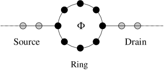
Figure 2: Schematic representation of a mesoscopic ring, threaded by a magnetic flux $\phi$, sandwiched symmetrically between the two reservoirs.

mesoscopic ring and thus we can say that the conductance spectrum manifests itself the electronic structure of the ring. From this figure it is observed that the resonant peaks get substantial widths (dotted line), compared to the weak-coupling case, as long as the coupling strength of the ring to the electrodes is increased.

Now we discuss the effect of external magnetic flux, threaded by the ring, on electron transport.

Figure 3: Conductance $g$ as a function of the injecting electron energy $E$ for a symmetrically connected mesoscopic ring ($N=30$) in the absence of any magnetic flux, where the solid and dotted lines correspond to the results for the weak- and strong-coupling limits, respectively.

In the presence of a magnetic flux, electron gains an additional phase, and accordingly, a constructive or destructive interference takes place after the electron propagation across the ring. Figure 4 gives the variation of the conductance as a function of $\phi$ for a particular energy, where (a) corresponds to the results for the weak-coupling limit and (b) denotes the results for the strong-coupling limit. Here we take the ring size $N=12$, as an illustrative example. The solid and dotted curves in the conductance spectra are associated with the typical energies $E=0.5$ and $1.5$, respectively. It is observed that the conductance varies periodically with $\phi$ showing $\phi_{0}$ flux-quantum periodicity.

The scenario of electron transfer through the ring becomes much more clearly visible by studying the current $I$ as a function of the applied bias voltage $V$.

Figure 4: $g$-$\phi$ spectra for a symmetrically connected mesoscopic ring ($N=12$), where the solid and dotted curves correspond to the results for the typical energies $E=0.5$ and $1.5$, respectively. (a) weak-coupling limit and (b) strong-coupling limit.

The variation of the current with the bias voltage is presented in Fig. 5 for a mesoscopic ring with size $N=30$, where (a) and (b) correspond to the weak- and strong-coupling cases, respectively. The solid, dotted and dashed lines represent the results for $\phi=0$, $0.4$ and $0.8$, respectively. The current is evaluated by the integration procedure of the transmission function $T$, where the transmission function varies exactly similar to that of the conductance spectrum since the relation $g=2T$ exists from the Landauer conductance formula. The shape and height of the current steps depend on the width of the resonant peaks. In the weak-coupling limit, the current shows a staircase-like behavior with sharp steps, which is associated with discrete nature of the resonances. It is also noticed that in the presence of a magnetic flux the current shows more steps (dotted and dashed curves) compared to the current in

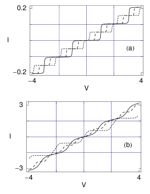
Figure 5: $I$-$V$ spectra for a symmetrically connected mesoscopic ring ($N=30$), where the solid, dotted and dashed curves correspond to the results for $\phi=0$, $0.4$ and $0.8$, respectively. (a) weak-coupling limit and (b) strong-coupling limit.

the absence of any magnetic flux (solid line). This is due the fact that more resonant peaks appear in the conductance spectrum in the presence of $\phi$. On the other hand, with the increase of the coupling strength, the current varies almost continuously with the applied bias voltage and achieves much larger values.

3.2 Ring sandwiched asymmetrically between the two reservoirs

The schematic view of an asymmetrically connected mesoscopic ring is shown in Fig. 6, where the upper and lower arms contain unequal number of atomic sites. The idea of considering such a geometry is that, in this way the interference condition can be changed nicely and the effect of ring-electrode interface geometry can be clearly understood. It can be analyzed in this way. The electrons are carried from the source to drain

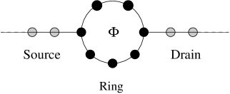
Figure 6: Schematic view of a mesoscopic ring, threaded by a magnetic flux $\phi$, attached asymmetrically between the two reservoirs.

through the ring and the electron waves propagating along the two arms of the ring may suffer a phase shift among themselves. This is due to the result of quantum interference between the waves passing through the

Figure 7: Conductance as a function of the energy $E$ for an asymmetrically connected mesoscopic ring with $N=30$, where the upper and lower arms contain $8$ and $20$ atomic sites, respectively. $\phi$ is set at $0$. The solid and dotted curves represent the results for the weak- and strong-coupling limits, respectively.

two arms of the ring. As a result, the probability amplitude of the electron across the ring may be strengthened or weakened, according to the standard theory of quantum mechanics. In Fig. 7, we plot the conductance as a function of energy in the absence of any magnetic flux $\phi$ for an asymmetrically connected mesoscopic ring, where the upper and lower arms contain $8$ and $20$ atomic sites, respectively. The solid and dotted curves correspond to the results for the weak- and strong-coupling limits, respectively. It is observed that both for the strong- and weak-coupling cases the resonant peaks do not reach to $2$ anymore, i.e., transmission probability does not reach to unity. This is due to the effect of interference of the electronic waves

Figure 8: $g$-$\phi$ characteristics for an asymmetrically connected mesoscopic ring with $N=12$, where the upper and lower arms contain $2$ and $8$ atomic sites, respectively. The solid and dotted curves represent the results for the typical energies $E=0.5$ and $1.5$, respectively. (a) weak-coupling limit and (b) strong-coupling limit.

propagating through the two arms of the ring. Like as in Fig. 3, here also the conductance peaks get substantial widths with the increase of coupling strength as shown by the dotted curve.

In the presence of $\phi$ in these asymmetrically connected rings, the conductance shows resonant and anti-resonant peaks, similar to that as shown in Fig. 4, but the widths and amplitudes of these peaks get modified significantly. Figure 8 shows the variation of the typical conductances as a function of flux $\phi$ for an asymmetrically connected ring, where the upper arm contains $2$ atomic sites and the lower arm contains $8$ atomic sites. The typical conductances for the energy $E=0.5$ are shown by the solid curves, while for the energy $E=1.5$ they are presented by the dotted curves. The results for the weak- and strong-coupling cases are shown in (a) and (b), respectively. It is noticed that the typical conductance varies periodically with $\phi$ exhibiting $\phi_{0}$ flux-quantum periodicity.

Now we discuss the effect of interference on the current-voltage characteristics for the asymmetrically connected ring. As representative example, in Fig. 9 we plot the current as a

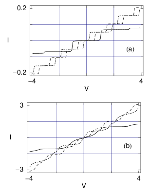
Figure 9: $I$-$V$ spectra for an asymmetrically connected ring with $N=30$, where the upper and lower arms have $8$ and $20$ atomic site, respectively. The solid, dotted and dashed curves correspond to the results for $\phi=0$, $0.4$ and $0.8$, respectively. (a) weak-coupling limit and (b) strong-coupling limit.

function of the bias voltage $V$ for an asymmetrically connected ring with $N=30$, where the upper and lower arms contain $8$ and $20$ atomic sites, respectively. The results for the weak- and strong-coupling limits are shown in (a) and (b), respectively, where the solid, dotted and dashed curves correspond to the identical meaning as in Fig. 5. In the absence of any magnetic flux $\phi$, the current amplitudes (solid curves) get reduced compared to the current amplitudes in the presence of $\phi$ (dotted and dashed curves) both for the weak- and strong-coupling limits. This is due to the geometric effect of the asymmetrically connected ring. In the weak coupling case, the current shows staircase-like behavior with sharp steps, similar to the symmetrically connected ring. Current shows more steps in the presence of $\phi$ than the current steps appear when $\phi$ becomes zero, since in the presence of $\phi$ more resonant peaks are obtained in the transmission spectrum. The current varies quite continuously for the strong-coupling limit and gets much higher values compared to the weak-coupling case, as expected from our previous discussion.

4 Concluding remarks

To summarize, we have addressed electron transport properties for some typical isolated mesoscopic rings using the Green’s function formalism. We have introduced a parametric approach based on the tight-binding model to characterize the transport properties in such systems. This technique can be used to study the electronic transport in any complicated systems, like complicated organic molecules, which bridge the two reservoirs. Both the ring-electrode interface geometry and the magnetic flux threaded by the ring have an important role on the electron transport since these two factors control the interference condition. We have also observed that the electron transport through the ring is significantly affected by the ring-to-electrode coupling strength. All these features may provide some basic inputs for fabrication of nanoscale devices.

References

- [1] V. Chandrasekhar, R. A. Webb, M. J. Brady, M. B. Ketchen, W. J. Gallagher, and A. Kleinsasser, Phys. Rev. Lett. 67, 3578 (1991).
- [2] D. Mailly, C. Chapelier, and A. Benoit, Phys. Rev. Lett. 70, 2020 (1993).
- [3] U. F. Keyser, C. Fühner, S. Borck, and R. J. Haug, Semicond. Sci. Technol. 17, L22 (2002).
- [4] A. Lorke, R. J. Luyken, A. O. Govorov, Jürg P. Kotthaus, J. M. Gracia, and P. M. Petroff, Phys. Rev. Lett. 84, 2223 (2000).
- [5] A. Fuhrer, S. Lüscher, T. Ihn, T. Heinzel, K. Ensslin, W. Wegscheiner, and M. Bichler, Nature (London) 413, 385 (2001).
- [6] A. I. Yanson, G. Rubio-Bollinger, H. E. van den Brom, N. Agraït, and J. M. van Ruitenbeek, Nature (London) 395, 780 (2001).
- [7] A. Aviram and M. Ratner, Chem. Phys. Lett. 29, 277 (1974).
- [8] S. N. Yaliraki, A. E. Roitberg, C. Gonzalez, V. Mujica, and M. A. Ratner, J. Chem. Phys. 111, 6997 (1999).
- [9] M. Di Ventra, S. T. Pantelides, and N. D. Lang, Phys. Rev. Lett. 84, 979 (2000).
- [10] Y. Xue, S. Datta, and M. A. Ratner, J. Chem. Phys. 115, 4292 (2001).
- [11] J. Taylor, H. Gou, and J. Wang, Phys. Rev. B 63, 245407 (2001).
- [12] P. A. Derosa and J. M. Seminario, J. Phys. Chem. B 105, 471 (2001).
- [13] P. S. Damle, A. W. Ghosh, and S. Datta, Phys. Rev. B 64, R201403 (2001).
- [14] V. Mujica, M. Kemp, and M. A. Ratner, J. Chem. Phys. 101, 6849 (1994).
- [15] V. Mujica, M. Kemp, A. E. Roitberg, and M. A. Ratner, J. Chem. Phys. 104, 7296 (1996).
- [16] M. P. Samanta, W. Tian, S. Datta, J. I. Henderson, and C. P. Kubiak, Phys. Rev. B 53, R7626 (1996).
- [17] M. Hjort and S. Staftröm, Phys. Rev. B 62, 5245 (2000).
- [18] K. Walczak, Cent. Eur. J. Chem. 2, 524 (2004).
- [19] K. Walczak, Phys. Stat. Sol. (b) 241, 2555 (2004).
- [20] W. Tian, S. Datta, S. Hong, R. Reifenberger, J. I. Henderson, and C. I. Kubiak, J. Chem. Phys. 109, 2874 (1998).
- [21] S. Datta, Electronic transport in mesoscopic systems, Cambridge University Press, Cambridge (1997).