Kondo screening coexisting with ferromagnetic order as a possible ground state for Kondo lattice systems

Abstract

We consider the competition between the Kondo screening effect and ferromagnetic long-range order (FLRO) within a mean-field theory of the Kondo lattice model for low conduction electron densities $n_{c}$. Depending on the parameter values, several types of FLRO ground states are found. When $n_{c}<0.16$, a polarized FLRO phase is dominant in the large Kondo coupling limit. For $0.16<n_{c}<0.82$, a non-polarized FLRO phase appears in the weak Kondo coupling region; while in the intermediate coupling region the ground state corresponds to the polarized and non-polarized FLRO phases, respectively, coexisting with the Kondo screening. For a strong Kondo coupling, the product of pure Kondo singlets is the ground state. Moreover, we also find that a weak magnetic field makes the pure Kondo singlet phase vanish, while the non-polarized FLRO state with the Kondo screening spans a large area in the phase diagram.

The Kondo lattice model is usually considered as a theoretical model for heavy fermion materials.Tsunetsugu1997 For this model, an important issue arises from the interplay between the Kondo screening and the magnetic interactions among local moments mediated by the conduction electrons, namely, the Ruderman-Kittel-Kasuya-Yosida (RKKY) exchange interaction. The former effect favors the formation of Kondo singlet state in the strong coupling limit, while the latter interactions tend to stabilize a magnetically long-range ordered state in the weak coupling limit. In-between these two distinct phases, there exists a quantum phase transition. The nature of such a transition has been a long standing issue since it was first suggested by Doniach.Doniach1977 In our earlier paper,Zhang2000a we proposed an extended mean field theory for an anisotropic Kondo lattice model with half-filled conduction electrons. Since the magnetic interactions and the Kondo screening were treated on an equal footing, we found that the disordered Kondo singlet state can coexist with antiferromagnetic long-range order (AFLRO) in the intermediate coupling regime, where the local moments are partially screened, resulting in a very small staggered magnetizations. These results have been confirmed in the whole AFLRO phase by quantum Monte Carlo calculations.Assaad2001 ; Ogata2007 Thus, the proposed extended mean-field theory can provide quite reliable physical results in the intermediate and strong Kondo coupling region.

So far most of the theoretical studies in this field focus on the antiferromagnetic heavy fermion materials. However, more and more heavy fermion metals with a ferromagnetic long-range order (FLRO) have been found experimentally: early examples are CePt_xSi,lee-ku-shelton CeRu₂Ge₂,Sullow-1999 CePt,Larrea CeSi_1.81,Drotziger CeAgSb₂,Sidorov and URu_2-xRe_xSi₂ at $x>0.3$ (Ref.Bauer-2005 ). Recently new ferromagnetic heavy fermion materials CeRuPO (Ref.Krellner ) and UIr₂Zn₂₀ (Ref. Bauer-2006 ) have been discovered. For some uranium compounds, the $S=1$ underscreened Kondo lattice model has been proposed to explain the coexistence of ferromagnetism and Kondo effect.Perkins To account for the FLRO state in the Kondo lattice model, we can actually assume that the density of conduction electrons per local moment $n_{c}$ is less than one, and then the FLRO states are more favorable energetically than the AFLRO state.Sigrist-1992 ; Li1996 The interplay between the Kondo screening and ferromagnetic long-range correlations is thus the most important issue. Another related essential problem is the nature of the Fermi surface,Si whether it is large, encompassing both the local moments and conduction electrons, or it is small, incorporating only the conduction electrons.

In this paper, motivated by the success of our previous investigation,Zhang2000a we will discuss these issues within the framework of a mean-field theory. By introducing the mean field order parameters, the FLRO and local Kondo screening effect can be treated on an equal footing, and we find several types of FLRO ground phases. In particular, for $0.16<n_{c}<0.82$, the ground state is a non-polarized FLRO phase in the weak coupling limit; while in the intermediate coupling regime the ground state can be polarized and non-polarized FLRO phases coexisting with a partial Kondo screening, depending on the Kondo coupling strength. In those FLRO phases without Kondo screening, the Fermi surface is a small one; while for those FLRO states with Kondo screening, the Fermi surface is a large one. Moreover, we also find that a weak magnetic field will make the pure Kondo singlet disordered state vanish and the non-polarized FLRO state with Kondo screening spanning a large area in the phase diagram.

The model Hamiltonian of the Kondo lattice systems is defined by

$$\mathcal{H}=\sum_{\mathbf{k},{\sigma}}\epsilon_{\mathbf{k}}c_{\mathbf{k}\sigma}^{\dagger}c_{\mathbf{k}\sigma}+J\sum_{i}\mathbf{\sigma}_{i}\cdot\mathbf{S}_{i}-\sum_{i}\mathbf{B}\cdot\left(\mathbf{\sigma}_{i}+\mathbf{S}_{i}\right),$$ (1)

where $\epsilon_{\mathbf{k}}$ is the dispersion of the conduction electrons, $\mathbf{\sigma}_{i}=\frac{1}{2}\sum_{{\alpha}\beta}c_{i\alpha}^{\dagger}\mathbf{\tau}_{\alpha\beta}c_{i\beta}$ is the spin density operator of the conduction electrons, $\mathbf{\tau}$ is the Pauli matrix, the Kondo coupling strength $J>0$, and a magnetic field couples equally to the local moments and conduction electrons. When the localized spins are represented by $\mathbf{S}_{i}=\frac{1}{2}\sum_{{\alpha}\beta}f_{i\alpha}^{\dagger}\mathbf{\tau}_{\alpha\beta}f_{i\beta}$ in the pseudo-fermion representation, the projection into the physical subspace has to be implemented by a local constraint $\sum_{\sigma}f_{i\sigma}^{\dagger}f_{i\sigma}=1$. It is straightforward to decompose the Kondo spin exchange into longitudinal and transversal parts

$$\mathbf{\sigma}_{i}\cdot\mathbf{S}_{i}=\sigma_{i}^{z}S_{i}^{z}-\frac{1}{4}[(c_{i\uparrow}^{\dagger}f_{i\uparrow}+f_{i\downarrow}^{\dagger}c_{i\downarrow})^{2}+(c_{i\downarrow}^{\dagger}f_{i\downarrow}+f_{i\uparrow}^{\dagger}c_{i\uparrow})^{2}],$$

where the longitudinal part describes the polarization of the conduction electrons, giving rise to the usual RKKY interaction between the local moments; while the transverse part represents the spin-flip scattering of the conduction by the local moments, yielding the local Kondo screening effect.Lacroix1979 The competition between these two interaction parts determines the possible ground state of the Kondo lattice systems. To correctly describe the ground state properties, both the Kondo screening effect and RKKY magnetic correlation should be treated on an equal footing.

To develop a simple mean field theory, we introduce FLRO order parameters: $m_{f}=\left\langle S_{i}^{z}\right\rangle$ and $m_{c}=\langle\sigma_{i}^{z}\rangle$ to decouple the longitudinal exchange term. Similarly, to describe the Kondo screening effect, a hybridization order parameter $V=\langle c_{i\uparrow}^{\dagger}f_{i\uparrow}+f_{i\downarrow}^{\dagger}c_{i\downarrow}\rangle$ is used to decouple the transverse exchange term. We also introduce a Lagrangian multiplier $\lambda$ to enforce the local constraint, which becomes the chemical potential in the mean field approximation. Then the mean field Hamiltonian in the momentum space can be written in a matrix form,

$$\mathcal{H}_{MF}=\sum_{\mathbf{k},{\sigma}}\left(c_{\mathbf{k}\sigma}^{\dagger},f_{\mathbf{k}\sigma}^{\dagger}\right)\left(\begin{array}[]{cc}\epsilon_{\mathbf{k}{\sigma}}&-\frac{JV}{2}\\ -\frac{JV}{2}&\lambda_{{\sigma}}\end{array}\right)\left(\begin{array}[]{c}c_{\mathbf{k}\sigma}\\ f_{\mathbf{k}\sigma}\end{array}\right)+\mathcal{N}\varepsilon_{0},$$ (2)

where $\epsilon_{\mathbf{k}{\sigma}}=\epsilon_{\mathbf{k}}+\frac{Jm_{f}-B}{2}{\sigma}$, $\lambda_{{\sigma}}=\lambda+\frac{Jm_{c}-B}{2}{\sigma}$, $\varepsilon_{0}=\frac{JV^{2}}{2}-Jm_{c}m_{f}-\lambda$, ${\sigma=\pm 1}$ denote the up and down spin orientations, and $\mathcal{N}$ is the total number of lattice sites. The quasiparticle excitation spectra are thus obtained by

$$E_{\mathbf{k}{\sigma}}^{\pm}=\frac{1}{2}\left[\epsilon_{\mathbf{k}{\sigma}}+\lambda_{{\sigma}}\pm\sqrt{\left(\epsilon_{\mathbf{k}{\sigma}}-\lambda_{{\sigma}}\right)^{2}+(JV)^{2}}\right],$$ (3)

where there appear four quasiparticle bands with spin splitting.

By using the method of equation of motion, we derive the following single particle Green functions

$$\langle\langle c_{\mathbf{k}\sigma}|c_{\mathbf{k}\sigma}^{\dagger}\rangle\rangle_{\omega}=\frac{\omega-\lambda_{{\sigma}}}{(\omega-\epsilon_{\mathbf{k}{\sigma}})(\omega-\lambda_{{\sigma}})-(\frac{JV}{2})^{2}},$$

$$\langle\langle f_{\mathbf{k}\sigma}|f_{\mathbf{k}\sigma}^{\dagger}\rangle\rangle_{\omega}=\frac{\omega-\epsilon_{\mathbf{k}{\sigma}}}{(\omega-\epsilon_{\mathbf{k}{\sigma}})(\omega-\lambda_{{\sigma}})-(\frac{JV}{2})^{2}},$$

$$\langle\langle f_{\mathbf{k}\sigma}|c_{\mathbf{k}\sigma}^{\dagger}\rangle\rangle_{\omega}=\langle\langle c_{\mathbf{k}\sigma}|f_{\mathbf{k}\sigma}^{\dagger}\rangle\rangle_{\omega}=\frac{-JV/2}{\omega-\lambda_{{\sigma}}}\langle\langle c_{\mathbf{k}\sigma}|c_{\mathbf{k}\sigma}^{\dagger}\rangle\rangle.$$ (4)

Accordingly, the corresponding density of states can be calculated and expressed as

$$\rho_{c}^{\sigma}(\omega)=\rho_{c}^{0}[\theta(\omega-\omega_{1\sigma})\theta(\omega_{2\sigma}-\omega)+\theta(\omega-\omega_{3\sigma})\theta(\omega_{4\sigma}-\omega)],$$

$$\rho_{f}^{\sigma}(\omega)=\left(\frac{JV/2}{\omega-\lambda_{{\sigma}}}\right)^{2}\rho_{c}^{\sigma}(\omega),$$

$$\rho_{f,c}^{\sigma}(\omega)=-\frac{JV/2}{\omega-\lambda_{{\sigma}}}\rho_{c}^{\sigma}(\omega),$$ (5)

where $\theta(\omega)$ is a step function. When the density of states of conduction electrons is assumed to be a constant $\rho_{c}^{0}=\frac{1}{2D}$ with $D$ as a half-width of the conduction electron band, the four quasiparticle band edges can be expressed as

$$\omega_{1\sigma} =\frac{1}{2}\left[\epsilon_{\sigma}-D+\lambda_{{\sigma}}-\sqrt{(\epsilon_{\sigma}-D-\lambda_{{\sigma}})^{2}+(JV)^{2}}\right],$$

$$\omega_{2\sigma} =\frac{1}{2}\left[\epsilon_{\sigma}+D+\lambda_{{\sigma}}-\sqrt{(\epsilon_{\sigma}+D-\lambda_{{\sigma}})^{2}+(JV)^{2}}\right],$$

$$\omega_{3\sigma} =\frac{1}{2}\left[\epsilon_{\sigma}-D+\lambda_{{\sigma}}+\sqrt{(\epsilon_{\sigma}-D-\lambda_{{\sigma}})^{2}+(JV)^{2}}\right],$$

$$\omega_{4\sigma} =\frac{1}{2}\left[\epsilon_{\sigma}+D+\lambda_{{\sigma}}+\sqrt{(\epsilon_{\sigma}+D-\lambda_{{\sigma}})^{2}+(JV)^{2}}\right],$$

where $\epsilon_{\sigma}=\frac{Jm_{f}-B}{2}{\sigma}$ and $\omega_{1\sigma}<\omega_{2\sigma}<\omega_{3\sigma}<\omega_{4\sigma}$.

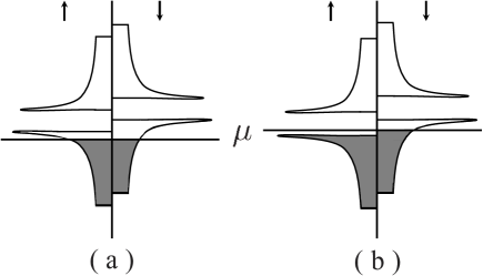
Figure 1: Schematic plot of total DOS in the presence of Kondo screening effect. (a) for the non-polarized FLRO phase, (b) for the polarized FLRO phase.

In the ground state, to keep the average numbers of $f$-electrons and conduction electrons equal to $1$ and $n_{c}$, respectively, the chemical potential $\mu$ has to be determined self-consistently. Therefore, the self-consistent equations determining the various mean-field parameters $m_{c}$, $m_{f}$, $V$, $\lambda$, and the chemical potential $\mu$ are given as follows

$$\left\{\begin{array}[]{c}n_{c}\\ 2m_{c}\\ 2V\\ 1\\ 2m_{f}\end{array}\right\}=\sum_{\mathbf{\sigma}}\int_{-\infty}^{+\infty}d\omega\rho_{c}^{\sigma}(\omega)\left\{\begin{array}[]{c}1\\ \sigma\\ -\frac{JV}{\omega-\lambda_{{\sigma}}}\\ \left(\frac{JV/2}{\omega-\lambda_{{\sigma}}}\right)^{2}\\ \sigma\left(\frac{JV/2}{\omega-\lambda_{{\sigma}}}\right)^{2}\end{array}\right\}.$$ (6)

Here the position of the chemical potential $\mu$ with respect to the band edges is an important factor. For $n_{c}<1$, there are two possible cases: $\omega_{1\downarrow}<\mu<\omega_{2\uparrow}$ and $\omega_{2\uparrow}<\mu<\omega_{2\downarrow}$. Moreover, we should assume that $n_{c}<0.82$ so that the RKKY interaction between the nearest neighboring local moments favors ferromagnetic coupling. Fazekas1991 Actually, the corresponding results for $1<n_{c}<2$ can be obtained via the particle-hole transformation $n_{c}\rightarrow\left(2-n_{c}\right)$ and $\sigma\rightarrow-\sigma$.

For $\omega_{1\downarrow}<\mu<\omega_{2\uparrow}$, the corresponding density of states is schematically shown in Fig. 1(a), where both the lower spin-up and spin-down quasiparticle bands are partially occupied. When we introduce the new variables,

$$x_{\sigma}=\lambda_{\sigma}-\mu\text{, }y_{\sigma}=\lambda_{\sigma}-\omega_{1\sigma},$$ (7)

the solution to the coupled self-consistent equations can be expressed in terms of $m_{c}$ and $m_{f}$

$$x_{\uparrow} =\frac{D(n_{c}+2m_{c})}{2\sinh(\frac{2D}{J})}\left[e^{-2D/J}+\sqrt{\frac{(n_{c}-2m_{c})(1-2m_{f})}{(n_{c}+2m_{c})(1+2m_{f})}}\right],$$

$$y_{\uparrow} =\frac{D(n_{c}+2m_{c})}{2\sinh(\frac{2D}{J})}\left[e^{2D/J}+\sqrt{\frac{(n_{c}-2m_{c})(1-2m_{f})}{(n_{c}+2m_{c})(1+2m_{f})}}\right],$$

$$x_{\downarrow} =\frac{D(n_{c}-2m_{c})}{2\sinh(\frac{2D}{J})}\left[e^{-2D/J}+\sqrt{\frac{(n_{c}+2m_{c})(1+2m_{f})}{(n_{c}-2m_{c})(1-2m_{f})}}\right],$$

$$y_{\downarrow} =\frac{D(n_{c}-2m_{c})}{2\sinh(\frac{2D}{J})}\left[e^{2D/J}+\sqrt{\frac{(n_{c}+2m_{c})(1+2m_{f})}{(n_{c}-2m_{c})(1-2m_{f})}}\right].$$ (8)

Considering the relation $x_{\downarrow}-x_{\uparrow}=B-Jm_{c}$ and the expressions for the quasiparticle band edges, we found a self-consistent equation for $m_{c}$,

$$\sqrt{n_{c}^{2}-4m_{c}^{2}+4(\eta-\alpha m_{c})^{2}}=\frac{\alpha(\alpha m_{c}-\eta)-m_{c}}{2m_{c}\sinh(2D/J)-\eta},$$ (9)

with $\alpha=\frac{J}{2D}\sinh\left(\frac{2D}{J}\right)-e^{-2D/J}$ and $\eta=\frac{B}{2D}\sinh(\frac{2D}{J})$. Solving Eq.(9) numerically will determine the magnetic order parameters $m_{c}$. Then $m_{f}$ can be calculated via

$$m_{f}=\frac{\eta-2m_{c}\sinh(2D/J)}{\alpha+m_{c}/(\eta-\alpha m_{c})},$$ (10)

and the other mean-field parameters can also be obtained from their equations as well.

However, when $\mathbf{B}=0$, we have $\eta=0$, and then analytical solutions to $m_{c}$ and $m_{f}$ can be derived as,

$$m_{c}=-\frac{1}{2}\sqrt{\frac{n_{c}^{2}-(\alpha\beta)^{2}}{1-\alpha^{2}}},m_{f}=-\frac{m_{c}}{\beta}$$ (11)

where $\beta=\frac{1-\alpha^{2}}{2\alpha\sinh(\frac{2D}{J})}$ and the hybridization parameter can be obtained

$$V^{2}=\frac{\cosh(\frac{2D}{J})\sqrt{\left(n_{c}^{2}-4m_{c}^{2}\right)(\beta^{2}-4m_{c}^{2})}+\beta n_{c}-4m_{c}^{2}}{2\beta\left(\frac{J}{2D}\sinh\frac{2D}{J}\right)^{2}}.$$ (12)

For $\omega_{2\uparrow}<\mu<\omega_{2\downarrow}$, the corresponding density of states is schematically shown in Fig. 1(b). Since the lower spin up quasiparticle band is completely occupied, we have $n_{c\uparrow}+n_{f\uparrow}=1$. But the lower spin down quasiparticle band is only partially occupied, the quasiparticles near the Fermi surface thus becoming polarized with a total magnetization

$$m_{c}+m_{f}=\frac{1-n_{c}}{2},$$ (13)

which corresponds to a plateau in the magnetization curve. Similarly, in terms of the new variables: $x_{\uparrow}=\lambda_{\uparrow}-\omega_{2\uparrow}$, $x_{\downarrow}=\lambda_{\downarrow}-\mu$, and $y_{\sigma}=\lambda_{\sigma}-\omega_{1\sigma}$, the solution to the coupled self-consistent equations can be derived in terms of $m_{c}$ and $m_{f}$

$$x_{\uparrow} =\frac{D(n_{c}+2m_{c})}{2\sinh(\frac{2D}{J})}\left[e^{-2D/J}+\sqrt{\frac{n_{c}-2m_{c}}{1+2m_{f}}}\right],$$

$$y_{\uparrow} =\frac{D(n_{c}+2m_{c})}{2\sinh(\frac{2D}{J})}\left[e^{2D/J}+\sqrt{\frac{n_{c}-2m_{c}}{1+2m_{f}}}\right],$$

$$x_{\downarrow} =\frac{D(n_{c}-2m_{c})}{2\sinh(\frac{2D}{J})}\left[e^{-2D/J}+\sqrt{\frac{1+2m_{f}}{n_{c}-2m_{c}}}\right],$$

$$y_{\downarrow} =\frac{D(n_{c}-2m_{c})}{2\sinh(\frac{2D}{J})}\left[e^{2D/J}+\sqrt{\frac{1+2m_{f}}{n_{c}-2m_{c}}}\right].$$ (14)

When the relations $y_{\uparrow}-x_{\uparrow}=D(n_{c}+2m_{c})$, $y_{\downarrow}-x_{\downarrow}=D(n_{c}-2m_{c})$, $m_{c}+m_{f}=\frac{1-n_{c}}{2}$, and the band edge expressions are taken into account, the final forms of the mean field order parameters can be obtained as

$$m_{c}=-\frac{\gamma\left(1-n_{c}\right)}{2\left(1-\gamma\right)},m_{f}=-\frac{m_{c}}{\gamma},$$

$$V^{2}=\frac{\cosh(\frac{2D}{J})\sqrt{\left(n_{c}-2m_{c}\right)(1+2m_{f})}+1-2m_{c}}{2(1-2m_{f})^{-1}\left(\frac{J}{2D}\sinh\frac{2D}{J}\right)^{2}},$$ (15)

where $\gamma$ has to be determined from the following equation self-consistently

$$\sqrt{\frac{n_{c}\left(1-2\gamma\right)+\gamma}{2-n_{c}-\gamma}}+\gamma\sqrt{\frac{2-n_{c}-\gamma}{n_{c}\left(1-2\gamma\right)+\gamma}}$$

$$=\alpha\left(1+\gamma\right)-2\gamma\sinh\left(\frac{2D}{J}\right).$$ (16)

Notice that this solution is independent of the external magnetic field and a constraint $\gamma<n_{c}$ has to be taken into account when solving Eq.(16) numerically.

Actually, it is easy to verify that the pure saturated FLRO state ($m_{f}=1/2$) without a hybridization can also be a solution to Eq. (12) and Eq. (15). However, our detailed calculations lead to the polarized and non-polarized FLRO phases, and we will call them polar-I and non-polar-I FLRO states, respectively, where the conduction electrons are partially or completely polarized by the saturated local moments with magnetizations

$$\text{ }m_{c}=\left\{\begin{array}[]{c}-\frac{n_{c}}{2},\text{ \ \ \ \ }n_{c}<\frac{J-2B}{4D}\\ -\frac{J-2B}{8D},\text{ \ \ }n_{c}>\frac{J-2B}{4D}\end{array}\right..$$ (17)

Obviously, the phase boundary between these two pure FLRO phases is given by $n_{c}=\frac{J-2B}{4D}$.

Similarly, it can also be noticed that the pure Kondo singlet phase ($m_{c}=m_{f}=0$ but $V\neq 0$) as a solution to the self-consistent equations requires $B=0$, namely, the pure Kondo singlet disordered state only exists in the absence of external magnetic field. The hybridization parameter of the Kondo screening is given by

$$V=\sqrt{n_{c}}\left(\frac{J}{D}\sinh\frac{D}{J}\right)^{-1}.$$ (18)

The boundary between the pure FLRO phase and FLRO coexisting with the Kondo screening effect should be described by the condition $V=0$.

In general, we have to employ the numerical calculations to solve Eq.(9) and Eq.(16), respectively. The ground-state phase diagram for $B=0$ is displayed in Fig. 2(a). Several types of FLRO ground states can be found. When $n_{c}<0.16$, the polar-I FLRO phase is dominant as a ground state in the large Kondo coupling region. For $0.16<n_{c}<0.82$, the ground state is given by the non-polar-I FLRO phase in the weak Kondo coupling limit; while in the intermediate Kondo coupling regime polarized and non-polarized FLRO phases with a finite value of the hybridization parameter $V$ appear separately, depending on the Kondo coupling strength. We will call them polar-II and non-polar-II FLRO states, respectively. For a strong Kondo coupling, the pure Kondo singlet phase is the ground state. The phase boundary between the polar-II and non-polar-II FLRO phases is given by $2(m_{c}+m_{f})=1-n_{c}$, and the hybridization parameter $V=0$ can be used to determine the phase boundaries between the polar-I and polar-II FLRO phases as well as for the polar-I and non-polar-II FLRO phases.

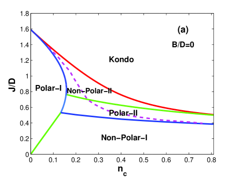
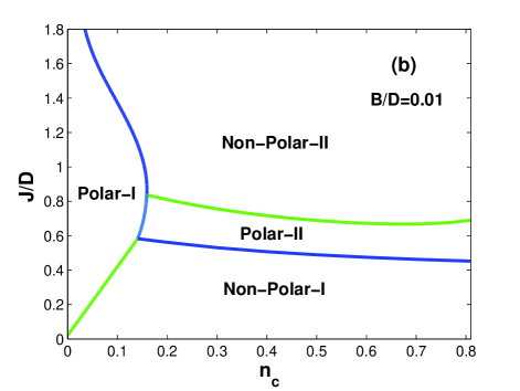
Figure 2: (Color online) Ground state phase diagram of the Kondo lattice model. (a) for B/D=0. The dashed line is given by comparing the ground state energies of the pure Kondo singlet and pure FLRO states. (b) for B/D=0.01.

For a given value of $n_{c}$, the mean field order parameters $m_{c}$, $m_{f}$, and $V$ as functions of the Kondo coupling strength are calculated and shown in Fig. 3(a). All the quantum phase transitions in the phase diagram are continuous second order, except for the phase transition from non-polar-I to the polar-II FLRO phases, because the hybridization parameter $V$ has a jump from zero to a finite value at the transition line. The phase boundary of this first-order transition is actually determined by comparing the two ground state energies, displayed in Fig. 4.

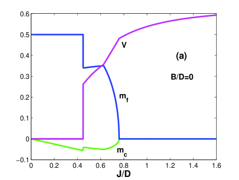
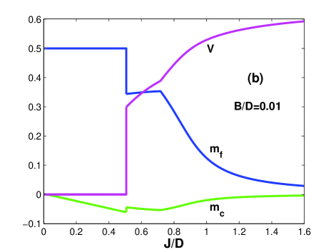
Figure 3: (color online) Mean field order parameters as functions of $J/D$ for $n_{c}=0.4$. (a) $B/D=0$, (b) $B/D=0.01$.

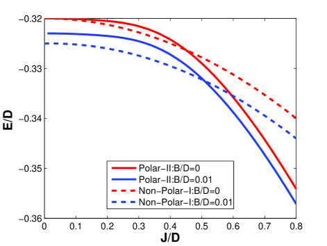
Figure 4: (color online) Comparison of the ground state energies of non-polar-I with polar-II FLRO phases in the absence and presence of a weak magnetic field for $n_{c}=0.4$.

The total magnetization $M$ as a function of the Kondo coupling strength for $n_{c}=0.4$ is shown in Fig.5, where a plateau appears in the curve with a fixed value of $(1-n_{c})/2$. The onset position of this plateau is just linked to the vanishing of the Fermi surface in the lower spin up quasiparticles.Beach2008 Thus, the presence of such a plateau can be used as an indication of the polarized quasiparticles near the Fermi surface.

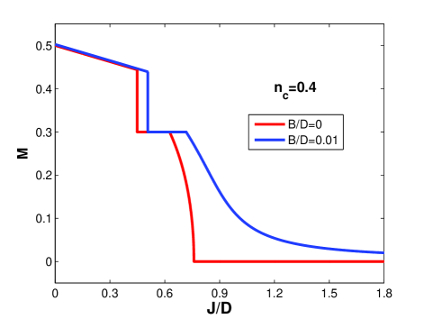
Figure 5: (color online) Total magnetization curve as a function of $J/D$ for a given value of $n_{c}$. A plateau appears when polarized quasiparticles are present near Fermi surface.

In the absence of the magnetic field, a very appealing physical picture emerges. In the pure polarized and non-polarized FLRO phases, the conduction electrons are decoupled from the local moments. For $0.16<n_{c}<0.82$, when $J/D$ is large enough, the localized moments are screened by the conduction electrons via the formation of local singlets, leading to a product of the local Kondo spin singlet disordered phase. It should be noticed that those conduction electrons in the Kondo singlets are not localized but itinerant so that the Kondo lattice system still displays metallic properties. As $J/D$ is in the intermediate coupling regime, the local moments are only partially screened by the conduction electrons, and the remaining uncompensated parts on the neighboring lattice sites develop the ferromagnetic long-range correlations mediated by the conduction electron spins, yielding the FLRO phases. The resulting FLRO states are either polarized or non-polarized, depending on the Kondo coupling strength. In these FLRO phases with Kondo screening, the quasiparticles consist of the conduction electrons and local moments, and the corresponding Fermi surface should be the large one. However, as $J/D$ becomes much smaller in the same density range, the local moments decoupled from the conduction electrons are aligned, forming the long-range order. In those FLRO phases without Kondo screening, the Fermi surface only involves the conduction electrons, corresponding to a small Fermi surface. Therefore, the hybridization between the conduction electrons and the $f$-electrons $V\neq 0$ or $V=0$ will determine whether the Fermi surface is large or small.

In the presence of a weak magnetic field, the mean field order parameters $m_{c}$, $m_{f}$, and $V$ as functions of the Kondo coupling strength are also calculated and shown in Fig. 3(b), where the pure Kondo singlet disordered phase vanishes completely. The corresponding phase diagram is displayed in Fig. 2(b). Generally speaking, in response to a weak magnetic field, the Zeeman splitting lifts the degeneracy of the spin up and spin down in the hybridization channel, shifting them with respect to one another and producing the magnetic moments. However, both polar-II and non-polar-II FLRO phases still have a small but finite value of $V$. Thus, the Kondo screening effect coexist with the FLRO phases in the large Kondo coupling regime. In contrary, it has been demonstrated that there is a critical magnetic field under which a Kondo singlet state persists in the Kondo insulating ground state with AFLRO correlations. Beach2004 ; Ohashi2004

In conclusion, due to the competition between the Kondo screening and magnetic RKKY interactions in the low density of the conduction electrons, a polar- and non-polar FLRO states can coexist with the Kondo screening both in the absence and presence of a weak magnetic field. These two phases should have large Fermi surfaces. On the other hand, the pure polar- and non-polar FLRO phases have small Fermi surfaces. The applied weak magnetic field makes the pure disordered Kondo singlet phase vanish. Moreover, there also exist two polarized FLRO phases with the total magnetization fixed by a value $M=(1-n_{c})/2$. To some extent, our present mean field theory captures the physics of the Kondo lattice systems with ferromagnetic correlations, especially the essence of the competition between Kondo screening effect and ferromagnetism. In order to put these mean field results on a solid ground, further investigations beyond the mean field theory are certainly needed.

This work is partially supported by NSF-China and the National Program for Basic Research of MOST, China.

References

- (1) H. Tsunetsugu, M. Sigrist, and K. Ueda, Rev. Mod. Phys. 69, 809 (1997), and references therein.
- (2) S. Doniach, Physica, B & C 91, 231 (1977).
- (3) G. M. Zhang and L. Yu, Phys. Rev. B 62, 76 (2000).
- (4) S. Capponi and F. F. Assaad, Phys. Rev. B 63, 155114 (2001).
- (5) H. Watanabe and M. Ogata, Phys. Rev. Lett. 99, 136401 (2007).
- (6) W. H. Lee, H. C. Ku, and R. N. Shelton, Phys. Rev. B 38, 11562 (1988).
- (7) S. Sullow, M. C. Aronson, B. D. Rainford, and P. Haen, Phys. Rev. Lett. 82, 2963 (1999).
- (8) J. Larrea, et. al., Phys. Rev. B 72, 035129 (2005).
- (9) S. Drotziger, et. al., Phys. Rev. B 73, 214413 (2006).
- (10) V. A. Sidorov, et. al., Phys. Rev. B 67, 224419 (2003).
- (11) E. D. Bauer, et. al., Phys. Rev. Lett. 94, 046401 (2005).
- (12) C. Krellner, et. al., Phys. Rev. B 76, 104418 (2007).
- (13) E. D. Bauer, et. al., Phys. Rev. B 74, 155118 (2006).
- (14) N. B. Perkins, J. R. Iglesias, M. D. Nunez-Regueiro, B. Coqblin, Eur. Phys. Lett. 79, 57006 (2007).
- (15) M. Sigrist, K. Ueda, and H. Tsunetsugu, Phys. Rev. B 46, 175 (1992).
- (16) Z. Z. Li, M. Zhuang, and M. W. Xiao, J. Phys.:Condens. Matter 8, 7941 (1996).
- (17) S. J. Yamamoto and Q. Si, arXiv:0812.0819.
- (18) C. Lacroix, and M. Cyrot, Phys. Rev. B 20, 1969 (1979).
- (19) P. Fazekas and E. Müller-Hartmann, Z. Phys. B 85, 285 (1991).
- (20) K. S. D. Beach and F. F. Assaad, Phys. Rev. B 77, 205123 (2008).
- (21) K. S. D. Beach, P. A. Lee, and P. Monthoux, Phys. Rev. Lett. 92, 26401 (2004).
- (22) T. Ohashi, A. Koga, S. Suga, and N. Kawakami, Phys. Rev. B 70, 245104 (2004).