Proof of the Feldman-Karlin Conjecture on the
Maximum Number of Equilibria in an
Evolutionary System

Abstract

Feldman and Karlin conjectured that the number of isolated fixed points for deterministic models of viability selection and recombination among $n$ possible haplotypes has an upper bound of $2^{n}-1$. Here a proof is provided. The upper bound of $3^{n-1}$ obtained by Lyubich et al. (2001) using Bézout’s Theorem (1779) is reduced here to $2^{n}$ through a change of representation that reduces the third-order polynomials to second order. A further reduction to $2^{n}-1$ is obtained using the homogeneous representation of the system, which yields always one solution ‘at infinity’. While the original conjecture was made for systems of viability selection and recombination, the results here generalize to viability selection with any arbitrary system of bi-parental transmission, which includes recombination and mutation as special cases. An example is constructed of a mutation-selection system that has $2^{n}-1$ fixed points given any $n$, which shows that $2^{n}-1$ is the sharpest possible upper bound that can be found for the general space of selection and transmission coefficients.  
 
Keywords: Feldman Karlin conjecture; selection; recombination; transmission; fixed points; equilibria; Bézout’s Theorem; homotopy method.  
 
To appear in Theoretical Population Biology, doi:10.1016/j.tpb.2010.02.007

1 Introduction

In a tribute issue to the late Sam Karlin, Feldman (2009) recounts their early collaborations (Feldman and Karlin, 1968; Karlin and Feldman, 1969; Karlin and Feldman, 1970a, b), and mentions a longstanding unsolved conjecture they proposed regarding the maximum number of isolated fixed points of the population genotype frequencies, under viability selection and recombination:

For the two-locus two-allele problem these considerations suggested a maximum of fifteen fixed points, and in our work with the symmetric viability model we demonstrated that fifteen was indeed realizable when recombination was present. Amazingly, to this day, our conjecture that the maximum number of equilibria in any $n$-chromosome viability system and for any recombination arrangement is $2^{n}-1$ has not been proven, although there are no counterexamples.

Here I provide a proof, through a modification of the approach used by Lyubich (1992). The proof also generalizes the result to other genetic processes besides recombination, in fact, to any arbitrary biparental transmission system, as described below. These results apply to systems of autosomal loci with discrete, non-overlapping generations, random mating, and constant viability selection.

2 The Model

The dynamical system considered here is represented by the recursion:

$$x_{i}^{\prime}=g_{i}({\bf x}):=\frac{\displaystyle 1}{\displaystyle\sum_{j,k=1}^{n}w_{jk}x_{j}x_{k}}\ \sum_{j,k=1}^{n}T_{ijk}w_{jk}x_{j}x_{k}$$ (1)

where

$i\in\{1,\ldots,n\}$

indexes the $n$ possible gamete genotypes (i.e. haplotypes);

$x_{1},\ldots,x_{i},\ldots x_{n}$

are the state variables, the frequencies of haplotypes in the population, so $x_{i}\geq 0$ and $\sum_{i=1}^{n}x_{i}=1$;

${\bf x}=\begin{pmatrix}x_{1}\\ \vdots\\ x_{n}\end{pmatrix}$

, ${\bf g}({\bf x})=\begin{pmatrix}g_{1}({\bf x})\\ \vdots\\ g_{n}({\bf x})\end{pmatrix}$;

$x_{i}^{\prime}$

is the frequency of haplotype $i$ in the next generation;

$w_{jk}=w_{kj}\geq 0$

is the fitness of the diploid genotype composed of haplotypes $j$ and $k$;

$T_{ijk}=T_{ikj}\geq 0$

is the probability that diploid genotype $jk$ produces gamete genotype $i$, so

$$\sum_{i=1}^{n}T_{ijk}=1\ \mbox{for each }j,k.$$

Perfect transmission is said to occur if gamete genotypes are identical to one or the other of the parental haplotypes in equal proportions:

$$T_{ijk}=\frac{1}{2}(\delta_{ij}+\delta_{ik}).$$

where $\delta_{ij}=1$ if $i=j$, $\delta_{ij}=0$ if $i\neq j$.

This recursion defines the map

$${\bf g}:\Delta^{n-1}\mapsto\Delta^{n-1}$$

on the $n-1$ dimensional simplex,

$$\Delta^{n-1}=\{{\bf x}\geq{{\bf 0}}\colon\sum_{i=1}^{n}x_{i}=1\}\subset\mathbb{R}^{n}.$$

The entries of the $n$ by $n^{2}$ matrix ${\left[\stackrel{{\scriptstyle}}{{T_{ijk}}}\right]}$ of transmission probabilities are determined by the biological processes that occur during genetic transmission. Recombination, mutation, gene conversion, segregation distortion, inversions, and all of their combinations, are all representable by sets of $T_{ijk}$. An absence of any transforming processes, and no segregation distortion, produces perfect transmission. In this absence of transformation processes, a multiple locus system is equivalent to a single locus system where each multilocus haplotype is formally a single allele.

Processes that are not covered by this framework include gene duplication and transposition, since the number of potential haplotypes becomes infinite. Also, infinite alleles models (Ewens, 2004, Sec. 3.6) are obviously not covered. Deletions, however, within a fixed set of genes, are representable by $T_{ijk}$ with finite $n$.

The set of all possible transmission matrices clearly includes many that do not correspond to any known biological processes, but this will be seen to be irrelevant, as the results apply to all transmission matrices.

3 Prior Work

Several previous studies prove results close to Feldman and Karlin’s conjecture. Moran (1963), at the tail end of his Conclusions, provides early insight into the question of how many isolated fixed points are possible in a system of selection and recombination, when he invokes Bézout’s Theorem (1779a):

The above discussion also raises the interesting theoretical question of how many stationary points the adaptive topography for two unlinked loci can have. It is clear that in trivial cases such stationary points can fill up a linear or a real continuum. This occurs when the $w_{ij}$ are independent of $i$, or $j$, or both. We may, however, ask how many isolated stationary points are possible. The two equations typified by (15) are cubics in $P$ and $p$ and hence, by Bézout’s theorem have at most 9 distinct isolated solutions, real or complex.

Tallis (1966) shows that with selection and perfect transmission, there are a maximum of $2^{n}-1$ isolated fixed points of ${\bf g}$, each fixed point being a population containing haplotypes from one of the $2^{n}-1$ possible subsets of $n$ haplotypes, the empty set excluded. (Also see Lyubich 1992, Theorem 9.1.1.)

Lyubich (1992) shows that with arbitrary transmission but with no selection, $2^{n-1}$ is an upper bound on the number of isolated fixed points of ${\bf g}$. Lyubich et al. (2001) show that with arbitrary transmission and selection, $3^{n-1}$ is an upper bound on the number of isolated fixed points of ${\bf g}$.

The approach taken in Lyubich (1992) and Lyubich et al. (2001) to obtain the upper bounds relies on Bézout’s Theorem (1779a).

As originally stated (translated from French):

Theorem 1.

Bézout (1779b, 47. p. 24) The degree of the final equation resulting from an arbitrary number of complete equations containing the same number of unknowns and with arbitrary degrees is equal to the product of the exponents of the degrees of these equations.

Here, the ‘final equation’ is a reference to the elimination method for solving systems of polynomials. An immediate application is:

Corollary 1.

Bézout (1779b, 48.3. p. 24) The number of intersection points of three surfaces expressed by algebraic equations is not greater than the product of the three exponents of the degrees of these equations.

The corollary is readily generalized to the intersection of arbitrary numbers of algebraic curves, to yield the version of Bézout’s theorem utilized here, restated from Kollár (2008, p. 365-366):

Theorem 2 (Bézout’s Theorem).

Let $f_{1}({\bf x}),\ldots,f_{n}({\bf x})$ be $n$ polynomials in $n$ variables, and for each $i$ let $d_{i}$ be the degree of $f_{i}$. Then either

1. the equation(s) $f_{1}({\bf x})=\cdots=f_{n}({\bf x})=0$ have at most $d_{1}d_{2}\cdots d_{n}$ solutions; or

2. the $f_{i}$ vanish identically on an algebraic curve $C$, and so there is a continuous family of solutions.

3.1 In the Absence of Selection

Bézout’s Theorem is applied as follows by Lyubich (1992, pp. 294-296). In the absence of selection, the system of fixed points of (1) can be written as the zeros of a system of polynomials:

$$0=f_{i}({\bf x}):=\sum_{j,k=1}^{n}T_{ijk}x_{j}x_{k}-x_{i}\ \ (i=1,\ldots,n-1)$$ (2)

and

$$0=f_{n}({\bf x}):=\sum_{i=1}^{n}x_{i}-1.$$ (3)

This gives $n-1$ equations of degree 2, and one equation of degree 1 ( (2) and (3), respectively). Therefore, ${\bf f}({\bf x})={{\bf 0}}$ can have at most $2^{n-1}*1=2^{n-1}$ isolated solutions, which are the fixed points of ${\bf g}$.

Lyubich (1992, Theorem 8.1.4 and Corollary 8.1.7, pp. 295-296) invokes the Poincaré-Hopf index theorem to reduce the upper bound to $2^{n-1}-1$ when ${\bf g}$ maps all points on the boundary in the direction of the interior of the simplex: i.e.,

$$\mbox{for }{\bf x} \in\partial\Delta^{n-1}\colon$$

$$(1-\epsilon)\ {\bf x}+\epsilon\ {\bf g}({\bf x})\in\Delta^{n-1}-\partial\Delta^{n-1}\mbox{\ for small \ }\epsilon>0,$$

or, more simply,

$$\mbox{if }x_{i}=0,\mbox{then }g_{i}({\bf x})>0.$$ (4)

Lyubich (1992, p. 295) provides inferences between several related conditions. Let ${\cal F}({\bf g})=\{\hat{{\bf x}}\colon{\bf g}(\hat{{\bf x}})=\hat{{\bf x}},\ \hat{{\bf x}}\in\Delta^{n-1}\}$ represent the set of fixed points of ${\bf g}$ on ${\Delta^{n-1}}$. The conditions are:

$${\cal F}({\bf g})\cap\partial\Delta^{n-1}=\emptyset;$$ (5)

$$\mbox{1 = Poincar\'{e}-Hopf index of }{\bf g}\mbox{\ on }\partial\Delta^{n-1};$$ (6)

$${\left[\stackrel{{\scriptstyle}}{{T_{ijj}}}\right]}_{i,j=1}^{n}\mbox{\ is an irreducible matrix};$$ (7)

$$T_{ijj}>0\ \forall\ i,j\in\{1,\ldots,n\};$$ (8)

$${\bf g}({\bf x})\in{\Delta^{n-1}}-\partial{\Delta^{n-1}},\ \forall{\bf x}\in{\Delta^{n-1}}.$$ (9)

Lyubich proposes the following chain of implications:

$$\eqref{cond:Interior}\iff\eqref{cond:PositiveHomozygous}\implies\eqref{cond:Irreducible}\implies\eqref{cond:BoundaryFree}\implies\eqref{eq:BoundaryCondition}\implies\eqref{cond:PHopf}$$

Additional consideration, however, shows the correct chain of implications to be:

$$\eqref{cond:Interior}\iff\eqref{cond:PositiveHomozygous}\left\{\begin{array}[]{l}\!\!\!\!\implies\eqref{cond:Irreducible}\implies\eqref{cond:BoundaryFree}\\ \\ \!\!\!\!\implies\eqref{eq:BoundaryCondition}\left\{\begin{array}[]{l}\!\!\!\!\implies\eqref{cond:BoundaryFree}\\ \!\!\!\!\implies\eqref{cond:PHopf}\end{array}\right.\end{array}\right.$$

In particular, $\eqref{cond:BoundaryFree}\ \ \not\!\!\!\!\implies\eqref{eq:BoundaryCondition}$. Lyubich writes, if “the boundary of the simplex contains no fixed points [(5)] then the vector field $Vx-x$ on the boundary is directed inside the simplex [(4)].” Following is a (nonbiological) counterexample where (5) and (7) hold, but (4) does not (without claiming the theorems themselves to be invalid): it is possible for the boundary to be without fixed points, and for the matrix $[T_{ijj}]$ to be irreducible (Lyubich uses the alternate term ‘indecomposable’), yet for ${\bf g}$ to map boundary points toward the boundary and not the interior.

Let $T$ simply rotate the index of each haplotype by -1:

$$T_{ijk}=\left\{\begin{array}[]{l l}1&\mbox{for \ \ }i\!\!\!\!\!\pmod{n}+1=j=k,\\ 1/2&\mbox{for \ \ }i\!\!\!\!\!\pmod{n}+1=j\neq k,\\ 1/2&\mbox{for \ \ }i\!\!\!\!\!\pmod{n}+1=k\neq j,\\ 0&\mbox{otherwise}.\end{array}\right.$$

An initial point ${\bf x}={\bf e}_{1}:=(1,0,\cdots,0)^{\top}$ ($\scriptstyle\top$, the transpose) is taken by ${\bf g}$ through a cycle of period $n$ through the vertices of the simplex, ${\bf e}_{1}$, ${\bf e}_{n}$, ${\bf e}_{n-1}$, $\ldots$, ${\bf e}_{2}$, ${\bf e}_{1}$, ${\bf e}_{n},\ldots$.

Every point on the boundary maps to a different point on the boundary. This can be seen because every boundary point must have some indices $i,i+1$ (modulo $n$) such that $x_{i}>0$ while $x_{i+1}=0$, but $T$ rotates the indices so that $g_{i}({\bf x})=0$ in the next generation, so no boundary point is fixed. Moreover, for any point on the boundary with adjacent zeroes, i.e. $x_{i}=x_{i+1}=0$, then $g_{i}({\bf x})=0$, contrary to boundary condition (4). Here, boundary points of a sub-simplex map to other boundary points of that sub-simplex, so $(1-\epsilon){\bf x}+\epsilon\,{\bf g}({\bf x})$ remains on the boundary for all $0\leq\epsilon\leq 1$. Any fixed points must therefore be in the interior of the simplex, and by symmetry, this can only be the center, ${\bf x}=(1/n,\ldots,1/n)^{\top}$. Thus, the exclusion of fixed points from the boundary does not imply that ${\bf g}$ maps the boundary in the direction of the interior.

What Lyubich is really after, however, is condition (6). So if one starts by assuming (4), then (6) follows and the rest of Lyubich’s proof goes through:

1. ${\bf g}$ has a Poincaré-Hopf index of 1 on the boundary of the simplex (6);

2. The index must equal the sum of the indices of the fixed points in the interior of the simplex (see Glass 1975b and Glass 1975a for an accessible explication of this approach);

3. The index of a non-degenerate fixed point must be $+1$ or $-1$;

4. Supposing that the maximum of $2^{n-1}$ fixed points is attained, then each must have multiplicity of 1, and is thus non-degenerate;

5. Having $2^{n-1}$ non-degenerate fixed points in the interior of the simplex, however, would produce a sum for their indices that is even, contrary to the index of ${\bf g}$ under condition (4);

6. So there can be no more than $2^{n-1}-1$ isolated fixed points of ${\bf g}$ in the interior of $\Delta^{n-1}$ given (4).

3.2 In the Presence of Selection

The above result is derived when selection is absent, and the only force acting is transmission of some arbitrary form. When selection is included along with transmission, the system of fixed points becomes:

$$0=f_{i}({\bf x}):=\sum_{j,k=1}^{n} T_{ijk}w_{jk}x_{j}x_{k}-x_{i}\sum_{j,k=1}^{n}w_{jk}x_{j}x_{k}$$ (10)

$$(i=1,\ldots,n-1),$$

and

$$0 =f_{n}({\bf x}):=\sum_{i=1}^{n}x_{i}-1.$$

The terms $x_{i}\sum_{j,k=1}^{n}w_{jk}x_{j}x_{k}$ in (10) are all of degree 3, so Lyubich et al. (2001, eq. (33)) apply Bézout’s Theorem to obtain an upper bound of $3^{n-1}$ on the number of isolated fixed points.

The vastly larger value for the upper bound when selection is present, $3^{n-1}$, versus $2^{n-1}$ when selection is absent, seems counterintuitive, and one suspects that $3^{n-1}$ can be sharpened.

4 Results

Closer examination of (10) finds that the equations are third order only due to the presence of a single common factor, the mean fitness $\overline{w}:=\sum_{j,k=1}^{n}w_{jk}x_{j}x_{k}$. Such a structure suggests potentials from a change in the representation. This is indeed the case, and the system can be made second order by introducing an additional variable $y$, and an additional equation that constrains $y$ to equal the mean fitness at equilibrium. The result is as follows:

Theorem 3 (Generalized Feldman-Karlin Conjecture).

Consider the evolutionary system with viability selection, random mating, and arbitrary transmission of $n$ possible haplotypes, represented by the map ${\bf g}$:

$$x_{i}^{\prime}=g_{i}(x_{1},\ldots,x_{n})=\frac{\displaystyle 1}{\displaystyle\sum_{j,k=1}^{n}w_{jk}x_{j}x_{k}}\ \sum_{j,k=1}^{n}T_{ijk}w_{jk}x_{j}x_{k}\ ,$$

where $i=1,\ldots,n$, $T_{ijk}\geq 0$, $\sum_{i=1}^{n}T_{ijk}=1$, $w_{ij}\geq 0$, and

$$x_{i}\geq 0,\ \sum_{i=1}^{n}x_{i}=1.$$ (11)

The number of isolated fixed points of ${\bf g}$ is never greater than $2^{n}-1$.

Proof.

With the introduction of an additional variable $y$, the system of fixed points can be represented as $n+1$ equations in $n+1$ variables:

$$0= \ f_{i}({\bf x},y):=\!\!\sum_{j,k=1}^{n}T_{ijk}w_{jk}x_{j}x_{k}-x_{i}y$$ (12)

$$(i=1,\ldots,n-1),$$

$$0= \ f_{n}({\bf x},y):=\sum_{j=1}^{n}x_{j}-1,$$ (13)

$$0= \ f_{n+1}({\bf x},y):=\sum_{i,j=1}^{n}w_{ij}x_{i}x_{j}-y.$$ (14)

Since all fixed points are isolated by hypothesis, application of Bézout’s Theorem to (12), (13), and (14) gives an upper bound of $2^{n-1}*1*2=2^{n}$ on the number of fixed points.

This comes within 1 of the value conjectured by Feldman and Karlin for the upper bound on the number of isolated fixed points of evolutionary systems (1). Their upper bound could be demonstrated if one could show that a solution satisfying (12), (13), and (14) always exists outside the simplex. Complex-valued solutions, and solutions ‘at infinity’, qualify and must be included in the count of solutions in Bézout’s Theorem.

A solution ‘at infinity’ is formally accounted for by mapping the system to projective space; this is accomplished by a homogeneous form for the intersection equations (Shafarevich, 1994, pp. 16-21). A new set of variables is defined:

$$z,$$

$$\overline{x}_{i}:=x_{i}\,z,\text{ and}$$

$$\overline{y}:=y\,z.$$

Substituting in (12), (13), and (14), one obtains $n+1$ equations in $n+2$ unknowns:

$$0= \ f_{i}({\bf x},y):=\frac{1}{z^{2}}\sum_{j,k=1}^{n}T_{ijk}w_{jk}\overline{x}_{j}\overline{x}_{k}-\frac{1}{z^{2}}\overline{x}_{i}\overline{y}$$ (15)

$$(i=1,\ldots,n-1),$$

$$0= \ f_{n}({\bf x},y):=\frac{1}{z}\sum_{j=1}^{n}\overline{x}_{j}-1,$$ (16)

$$0= \ f_{n+1}({\bf x},y):=\frac{1}{z^{2}}\sum_{i,j=1}^{n}w_{ij}\overline{x}_{i}\overline{x}_{j}-\overline{y}/z.$$ (17)

Multiplying both sides of (15) and (17) $z^{2}$, and (16) by $z$, one obtains the homogeneous form:

$$0= \ \overline{f}_{i}(\overline{{\bf x}},\overline{y},z):=\sum_{j,k=1}^{n}T_{ijk}w_{jk}\overline{x}_{j}\overline{x}_{k}-\overline{x}_{i}\overline{y}$$ (18)

$$(i=1,\ldots,n-1),$$

$$0= \ \overline{f}_{n}(\overline{{\bf x}},\overline{y},z):=\sum_{j=1}^{n}\overline{x}_{j}-z,$$ (19)

$$0= \ \overline{f}_{n+1}(\overline{{\bf x}},\overline{y},z):=\sum_{i,j=1}^{n}w_{ij}\overline{x}_{i}\overline{x}_{j}-\overline{y}\ z.$$ (20)

In the homogeneous representation, any non-trivial solution, $(\overline{{\bf x}},\overline{y},z)\neq({{\bf 0}},0,0)$, gives as solutions all its scalar multiples $c\,(\overline{{\bf x}},\overline{y},z)$, $c\in\mathbb{C}$. Hence all scalar multiples of a solution count as a single point (a point in projective space) when counting solutions.

The original system (12) is obtained by setting $z=1$. By setting $z=0$, any nontrivial solution ($\overline{{\bf x}}\neq{{\bf 0}}$ or $\overline{y}\neq 0$) corresponds to a solution ‘at infinity’ for (12), (13), and (14), since it would give ${\bf x}=\overline{{\bf x}}/0$ and $y=\overline{y}/0$.

Letting $z=0$ and $\overline{{\bf x}}={{\bf 0}}$, we see that this is a solution:

$$\overline{f}_{i}({{\bf 0}},\overline{y},0)= \sum_{j,k=1}^{n}T_{ijk}w_{jk}0*0-0\overline{y}=0$$

$$(i=1,\ldots,n-1),$$

$$\overline{f}_{n}({{\bf 0}},\overline{y},0)= \sum_{j=1}^{n}0-0=0,$$

$$\overline{f}_{n+1}({{\bf 0}},\overline{y},0)= \sum_{i,j=1}^{n}w_{ij}*0*0-\overline{y}\ 0=0.$$

The variable $\overline{y}$ is clearly unconstrained here, hence, the non-trivial solution is:

$$(\overline{{\bf x}},\overline{y})=c\,({{\bf 0}},1),\ c\neq 0.$$

This solution ‘at infinity’ reduces by $1$ the number of possible finite-valued fixed points, leaving an upper bound of $2^{n}-1$ on the number of isolated fixed points in the simplex $\Delta^{n-1}$. ∎

An illustration of how the solution ‘at infinity’ arises is given in section 5.1.

5 A Mutation-Selection System Bearing $2^{n}-1$ Isolated Fixed Points

Here, I show that $2^{n}-1$ is the smallest possible upper bound on the number of isolated fixed points for the general space of selection-transmission systems (1), by constructing an example that attain this bound. It is already known that the bound is attained by examples of systems with selection and perfect transmission, where one fixed point is located in the interior of the simplex and in the interior of each sub-simplex on the boundary, including the vertices (Tallis, 1966). So what remains to be determined is whether this bound can also be attained under some form of imperfect transmission.

Such systems can be produced through the homotopy continuation method (Kotsffeas, 2001; Li, 2003), where one creates a continuous family of systems between a known system, and an unknown system with desired properties. In this case, the homotopy will go from a known system of selection and perfect transmission that has $2^{n}-1$ fixed points, to systems with imperfect transmission, by perturbing the transmission probabilities. Under proper conditions, the homotopy will produce paths from the fixed points of the known system to the fixed points of unknown systems.

The homotopy continuation method per se originated independently in the work of Garcia and Zangwill (1977), Drexler (1977), and Chow et al. (1978) (Li, 1997). An essential part of this method can be found earlier in the ‘method of small parameters’ of Karlin and McGregor (1972b; 1972c; 1972a):

Principle I [if a system of transformations acting on a certain set (in finite dimensional space) has a “stable” fixed point, then a slight perturbation of the system maintains a stable fixed point nearby] can be interpreted as a perturbation or continuity theorem. Starting with a given genetic system for which the nature of the equilibria can be fully delineated (for example, the classical multi-allelic viability model), it is desired to investigate a perturbed version of the model. (1972b, p. 86)

Karlin and McGregor (1972c, Theorem 4.4, p. 231) use the implicit function theorem to establish the existence, uniqueness, and nearness of fixed points under perturbed models. The stability properties of the fixed points also are preserved by the additional assumption that all fixed points are hyperbolic. Hyperbolicity is not needed, however — only non-degeneracy — to establish the existence, uniqueness, and nearness of isolated fixed points (Akin, 1983, p. 24).

For the choice of the system to perturb, I use (1) with perfect transmission, which is formally a one-locus, multiple-allele system:

$$x_{i}^{\prime}=g_{i}({\bf x}):=\frac{\displaystyle 1}{\displaystyle\sum_{j,k=1}^{n}w_{jk}x_{j}x_{k}}\ x_{i}\sum_{j=1}^{n}w_{ij}x_{j}$$ (21)

Tallis (1966) gives two examples of (21) with $2^{n}-1$ fixed points, a fully overdominant and a fully underdominant system. The fully overdominant system is due to Wright (1949) (discussed in Li 1955, p. 260), and has $w_{ii}=1-s_{i}$, $w_{ij}=1$ for all $i\neq j$, where $0<s_{i}\leq 1$. The fully underdominant system has $w_{ii}=1$, $w_{ij}=1-s$ for all $i\neq j$, where $0<s_{i}\leq 1$.

The homotopy is created by perturbing perfect transmission using uniform mutation:

$$T_{ijk}=(1-\mu)\frac{1}{2}(\delta_{ij}+\delta_{ik})+\mu/n,$$ (22)

where $\mu$ is the mutation rate. With $\mu>0$, (22) satisfies conditions (9) and (8), yielding conditions (4), (5) and (6). Thus none of the boundary fixed points under (21) can remain on the boundary for $\mu>0$.

To keep all $2^{n}-1$ fixed points in the simplex when $\mu>0$, the fixed points of (21) on the boundary need to move inside the simplex. Since ${\bf g}$ points into the simplex for $\mu>0$, toward these fixed points, they need to have stable manifolds (Wiggins, 1990, pp. 193–239) that enter the simplex. A situation that produces this is where all $n$ corners of ${\Delta^{n-1}}$ are stable sink nodes, and all $k$-allele ($k\in\{2,\ldots,n-1\}$) polymorphic boundary fixed points are unstable source nodes with respect to the sub-simplex ${\Delta^{k-1}}$ for which they are interior points. Kingman (1961, p. 578) showed that under (21), the vertex equilibria are stable and all polymorphic equilibria unstable if ${\bf W}$ is positive definite. This is the case with the fully underdominant system (Also see Christiansen 1990.).

Let the fitnesses be $w_{ij}=1+s\,\delta_{ij}$, where $s>0$. In (21), the fixed points comprise: the vertices of the simplex; the centers of each $h-1$ dimensional sub-simplex on the boundary; and the center of the simplex. Fixed points will be of the form

$$(\underbrace{1/h,\ldots,1/h}_{h},\underbrace{0,\ldots,0}_{n-h})$$ (23)

in any of ${{n}\choose{h}}$ distinct permutations of the order, where $h$ varies from $1$ to $n$. Hence the number of fixed points is $\sum_{h=1}^{n}{{n}\choose{h}}=2^{n}-1$.

Letting the mutation rate $\mu$ become positive, this system provides a constructive proof for the following:

Theorem 4.

The upper bound of $2^{n}-1$ on the number of isolated fixed points for evolutionary systems (1) is sharp over the general space of selection and transmission coefficients. In particular, for any $n$, a system with imperfect transmission can be constructed that attains the upper bound of $2^{n}-1$ fixed points in the simplex, using $w_{ij}=1+s\,\delta_{ij}$, $s>0$, and

$$T_{ijk}=(1-\mu)\frac{1}{2}(\delta_{ij}+\delta_{ik})+\mu/n,$$

for the ranges $0<\mu<1/2$ and $s\geq\frac{\displaystyle n}{\displaystyle 1/\mu-2},$ yielding:

$$g_{i}({\bf x})= \frac{1}{1+s\sum_{j=1}^{n}x_{j}^{2}}$$ (24)

$$\left[(1-\mu)x_{i}+\frac{\mu}{n}+s(1-\mu)x_{i}^{2}+\frac{s\mu}{n}\sum_{j=1}^{n}x_{j}^{2}\right].$$

Proof.

For small $\mu$, (24) is a perturbation of the system with perfect transmission, so its fixed points will be close to the isolated and non-degenerate points (23). By symmetry we can expect them to be of the form:

$$\hat{{\bf x}}=P(\ \underbrace{\frac{1-a}{h},\ldots,\frac{1-a}{h}}_{h},\ \underbrace{\frac{a}{n-h},\ldots,\frac{a}{n-h}}_{n-h}\ )$$ (25)

for $h=1,\ldots,n-1$, where $P$ is any permutation of the order of the entries. For $h=n$ or $h=0$, $\hat{x}_{i}=1/n$ for all $i$.

To verify this form, and solve for $a$, we substitute into (24):

$$\frac{1-a}{h}(1+sV)$$

$$\displaystyle=(1-\mu)\frac{1-a}{h}+\frac{\mu}{n}+s(1-\mu)\left(\frac{1-a}{h}\right)^{2}+\frac{s\mu}{n}V$$

where

$$V:=\sum_{j=1}^{n}x_{j}^{2} =h\frac{(1-a)^{2}}{h^{2}}+(n-h)\frac{a^{2}}{(n-h)^{2}}$$

$$=\frac{(1-a)^{2}}{h}+\frac{a^{2}}{(n-h)},$$

which yields three roots:

$$a =1-h/n,$$

and

$$a= \frac{1}{2}+\mu\left(\frac{1}{2}-\frac{h}{n}\right)$$

$$\pm\sqrt{\left[\frac{1}{2}+\mu\left(\frac{1}{2}-\frac{h}{n}\right)\right]^{2}-\frac{\mu(h+s)(n-h)}{ns}}.$$

The first root yields the central equilibrium $x_{i}=1/n$. Substitution shows that the other two roots yield the two equilibrium forms in (25), where $h$ and $n-h$ are interchanged. The term inside the radical must be non-negative for real solutions, and so imposes constraints on $\mu$ and $s$:

$$\gamma(h) :=\left[\frac{1}{2}+\mu\left(\frac{1}{2}-\frac{h}{n}\right)\right]^{2}-\frac{\mu(h+s)(n-h)}{ns}$$ (26)

$$=\left(\frac{1}{2}-\frac{h}{n}\right)^{2}\left(\mu+\frac{n}{s}\right)\mu+\frac{1}{4}-\frac{\mu n}{4s}-\frac{\mu}{2}\geq 0.$$

To obtain the conditions for $\gamma(h)\geq 0$, first the value of $h$ is found that minimizes $\gamma(h)$:

$$\frac{d}{dh}\gamma(h)=-\frac{2}{n}\left(\frac{1}{2}-\frac{h}{n}\right)\left(\mu+\frac{n}{s}\right)\mu$$

So $\frac{d}{dh}\gamma(h)=0$ at $h=n/2$. The second derivative,

$$\frac{d^{2}}{dh^{2}}\gamma(h)=\frac{2}{n^{2}}\left(\mu+\frac{n}{s}\right)\mu,$$

is positive, hence $\gamma(n/2)$ is a minimum:

$$\gamma(n/2) =\left(\frac{1}{2}-\frac{1}{2}\right)^{2}\left(\mu+\frac{n}{s}\right)\mu+\frac{1}{4}-\frac{\mu n}{4s}-\frac{\mu}{2}$$

$$=\frac{1}{4}-\frac{\mu n}{4s}-\frac{\mu}{2}$$

Therefore,

$$\gamma(n/2)\geq 0\ \iff\ \frac{1}{4}\geq\mu\left(\frac{n}{4s}+\frac{1}{2}\right)$$

$$\iff\ \mu<1/2\mbox{ and }s\geq\frac{\mu\,n}{1-2\mu}.$$

If $n$ is odd, then the requirement is $\gamma(\frac{n+1}{2})=\gamma(\frac{n-1}{2})\geq 0$, but since $\gamma(n/2)$ is the minimum, the above constraints on $\mu$ and $s$ are sufficient to keep $\gamma(\frac{n+1}{2})$ non-negative. In (26), since $\mu(h+s)(n-h)/(ns)>0$, then $\sqrt{\gamma(h)}<\frac{1}{2}+\mu\left(\frac{1}{2}-\frac{h}{n}\right)$ so $a>0$, as required.

The number of fixed points is the number of permutations of (25), $2^{n}-1$, the same as for (23) with perfect transmission.

Therefore, ${\bf g}$ in (24) is an example of a system with imperfect transmission that attains the upper bound of $2^{n}-1$ isolated fixed points, all in the interior of the simplex. Thus, for the general space of fitness and transmission coefficients, the upper bound in Theorem 3 is sharp and cannot be lowered. ∎

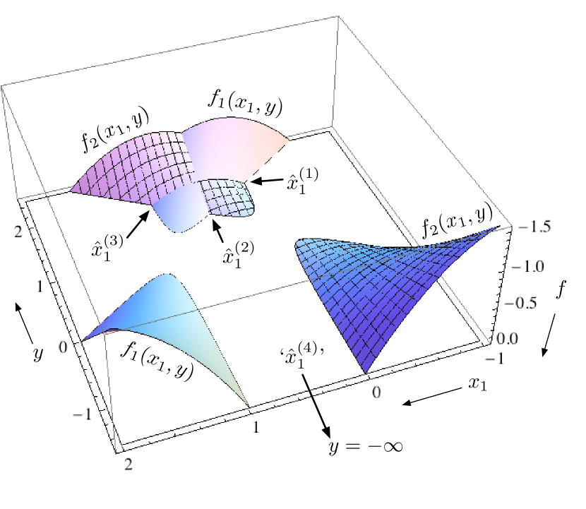
Figure 1: A plot of the polynomials (12) for the example (24) with $n=2$, $s=1$, $w_{11}=w_{22}=2$, $w_{12}=w_{21}=1$, and $\mu=0.05$. The range is truncated at 0 to show the curves of solutions to $f_{i}(x_{1},y)=0$. Shown are the three points of intersection, where $f_{1}(\hat{x}_{1}^{(k)},y^{(k)})=f_{2}(\hat{x}_{1}^{(k)},y^{(k)})=0$, for $k=1,2,3$. At those three points, $\overline{w}=y^{(k)}$. Counting as the fourth intersection ‘at infinity’, ‘$\hat{x}_{1}^{(4)}$’ indicates where the two curves approach parallel lines as $y\rightarrow-\infty$.

5.1 The Solution ‘At Infinity’

This example system is also useful to understand the nature of the $2^{n}$-th solution ‘at infinity’ in Bézout’s Theorem. Fig. 1 shows the polynomials (12) for the two-allele case. The two algebraic surfaces intersect each other and the $f_{i}=0$ plane at $2^{2}-1=3$ points. The absence of a fourth point is because the two algebraic surfaces approach parallel lines along the $f_{i}=0$ plane as $y$ goes to $-\infty$. These parallel lines are said to ‘meet at infinity’ when the system is represented in projective space using the homogeneous form (20).

6 Discussion

Theorem 3 proves the conjecture of Feldman and Karlin on the maximum number of isolated fixed points in a system of selection and recombination, and extends it to arbitrary transmission processes, of which recombination and mutation represent special cases. This substantially sharpens the previous upper bound of $3^{n-1}$ (Lyubich et al., 2001) on the number of isolated fixed points of an evolutionary system with selection and arbitrary transmission.

No attempt has been made to characterize the conditions on $T_{ijk}$ and $w_{jk}$ that produce only isolated and non-degenerate fixed points. More on this issue can be found in Lyubich et al. (2001). One may mention, however, that such conditions are generic, in that for ‘almost all’ sets of $n$ algebraic hypersurfaces of degree $n$, the intersection consists of isolated non-degenerate fixed points (Shafarevich 1994, p. 223, Garcia and Li 1980); and sets of $T_{ijk}$ values that produce degenerate fixed points are nowhere dense (Lyubich, 1992, Theorem 8.1.3) in the space of $T_{ijk}$ values. Recombination-only systems without selection exhibit only continua of fixed points with no isolated fixed points, because arbitrary allele frequencies are all invariant, and only linkage disequilibria change in time. Certain non-generic selection regimes also yield continua of fixed points.

The present paper does not touch at all upon the question of the stability of the equilibria. Studies on the stability of equilibria include the papers cited previously, and, as a selected additional list, Feldman et al. (1974), Karlin (1975), Karlin and Liberman (1976), Feldman and Liberman (1979), Karlin (1979), Karlin (1980), Hastings (1981), Hastings (1985), Franklin and Feldman (2000), and Puniyani and Feldman (2006).

It is notable that when selection is removed from the evolutionary system (1), the upper bound on the number of isolated fixed points decreases by half, from $2^{n}-1$ to $2^{n-1}$ ($2^{n-1}-1$ when condition (4) holds). In contrast, removing arbitrarily complicated imperfect transmission from (1) to constrain the systems to form (21), where only selection acts, does not reduce the potential number of isolated fixed points at all.

Removing selection means setting the $n\,(n+1)/2$ independent values of $w_{ij}$ to 1, whereas removing imperfect transmission means setting the $(n-1)\,n\,(n+1)/2$ independent values of $T_{ijk}$ to $(\delta_{ij}+\delta_{ik})/2$. Hence, paradoxically, when the ${\cal O}(n^{2})$ fitness coefficients are allowed to vary, it doubles the potential number of isolated fixed points, whereas when the ${\cal O}(n^{3})$ transmission probabilities are allowed to vary, the potential number of fixed points remains unchanged. This reveals a structural difference between the roles of selection and transmission in the dynamics.

A homotopy of a continuous family of evolutionary systems can be defined between any two evolutionary systems (1), in particular between ones with and without selection through the parameterizations:

$$w_{ij}(\alpha)=(1-\alpha)+\alpha\ w_{ij},\mbox{\ or \ }w_{ij}(\alpha)=w_{ij}^{\alpha}.$$

So any system

$$g_{i}^{(\alpha)}({\bf x}):=\frac{\displaystyle 1}{\displaystyle\sum_{j,k=1}^{n}w_{jk}(\alpha)\ x_{j}\ x_{k}}\ \sum_{j,k=1}^{n}T_{ijk}\ w_{jk}(\alpha)\ x_{j}\ x_{k}$$

with greater than $2^{n-1}$ fixed points will exhibit bifurcations of fixed points for some value(s) of $\alpha\in[0,1]$.

One can contemplate many other possible applications of the homotopy method to investigate the equilibrium behavior of these evolutionary systems.

7 Acknowledgments

The idea of creating a new variable to reduce the third order equations to second order came to me after seeing the use of substitutions in Brown (2009).

References

- Akin (1983) Akin, E., 1983. Hopf bifurcation in the two-locus genetic model. Memoirs of the American Mathematical Society 44 (284), 1–190.
- Bézout (1779a) Bézout, E., 1779a. Théorie Générale des Équations Algébriques. Pierres, Rue S. Jaques, Paris.
- Bézout (1779b) Bézout, E., 1779b. General Theory of Algebraic Equations (2006 translation by Eric Feron). Princeton University Press, Princeton.
-
Brown (2009)
Brown, K. S., 2009. The resultant and Bezout’s Theorem. MathPages.
URL www.mathpages.com/home/kmath544/kmath544.htm - Chow et al. (1978) Chow, S.-N., Mallet-Paret, J., Yorke, J. A., 1978. Finding zeroes of maps: Homotopy methods that are constructive with probability one. Mathematics of Computation 32 (143), 887–899.
- Christiansen (1990) Christiansen, F. B., 1990. The generalized multiplicative model for viability selection at multiple loci. Journal of Mathematical Biology 29 (2), 99–130.
- Drexler (1977) Drexler, F. J., 1977. Eine methode zur berechnung sämtlicher lösungen von poly- nomgleichungssystemen. Numer. Math. 29, 45–58.
- Ewens (2004) Ewens, W. J., 2004. Mathematical Population Genetics. I. Theoretical Introduction, 2nd Edition. Springer-Verlag, Berlin.
- Feldman (2009) Feldman, M. W., 2009. Sam Karlin and multi-locus population genetics. Theoretical Population Biology 75, 233–235.
- Feldman et al. (1974) Feldman, M. W., Franklin, I., Thomson, G. J., 1974. Selection in complex genetic systems I. the symmetric equilibria of the three-locus symmetric viability model. Genetics 76, 135–162.
- Feldman and Karlin (1968) Feldman, M. W., Karlin, S., 1968. Linkage and selection, new results for the two locus symmetric viability model. Genetics 60, 176.
- Feldman and Liberman (1979) Feldman, M. W., Liberman, U., 1979. On the number of stable equilibria and the simultaneous stability of fixation and polymorphism in two-locus models. Genetics 92, 1355–1360.
- Franklin and Feldman (2000) Franklin, I. R., Feldman, M. W., 2000. The equilibrium theory of one- and two-locus systems. In: Singh, R. S., Krimbas, C. B. (Eds.), Evolutionary Genetics: From Molecules to Morphology. Cambridge University Press, Cambridge, pp. 258–283.
- Garcia and Li (1980) Garcia, C. B., Li, T.-Y., 1980. On the number of solutions to polynomial systems of equations. SIAM Journal of Numerical Analysis 17 (4), 540–546.
- Garcia and Zangwill (1977) Garcia, C. B., Zangwill, W. I., 1977. Finding all solutions to polynomial systems and other systems of equations. Tech. Rep. 7738, Center for Mathematical Studies in Business and Economics, Dept. of Economics and Graduate School of Business University of Chicago, Chicago.
- Glass (1975a) Glass, L., 1975a. Combinatorial and topological methods in nonlinear chemical kinetics. The Journal of Chemical Physics 63 (4), 1325–1335.
- Glass (1975b) Glass, L., 1975b. A topological theorem for nonlinear dynamics in chemical and ecological networks. Proceedings of the National Academy of Sciences U.S.A. 72 (8), 2856–2857.
- Hastings (1981) Hastings, A., 1981. Stable cycling in discrete-time genetic models. Proceedings of the National Academy of Sciences U.S.A. 78, 7224–7225.
- Hastings (1985) Hastings, A., 1985. Four simultaneously stable polymorphic equilibria in two-locus two-allele models. Genetics 109 (1), 255–261.
- Karlin (1975) Karlin, S., 1975. General two-locus selection models. some objectives, results, and interpretations. Theoretical Population Biology 7, 364–398.
- Karlin (1979) Karlin, S., 1979. Principles of polymorphism and epistasis for multilocus systems. Proceedings of the National Academy of Sciences U.S.A. 76, 541–545.
- Karlin (1980) Karlin, S., 1980. The number of stable equilibria for the classical one-locus multi-allele selection model. Journal of Mathematical Biology 9, 189–192.
- Karlin and Feldman (1969) Karlin, S., Feldman, M. W., 1969. Linkage and selection: new equilibrium properties of the two-locus symmetric viability model. Proc. Natl. Acad. Sci. USA 62, 70–74.
- Karlin and Feldman (1970a) Karlin, S., Feldman, M. W., 1970a. Convergence to equilibrium of the two locus additive viability model. J. Applied Probability 7, 262–271.
- Karlin and Feldman (1970b) Karlin, S., Feldman, M. W., 1970b. Linkage and selection: two locus symmetric viability model. Theoretical Population Biology 1, 39–71.
- Karlin and Liberman (1976) Karlin, S., Liberman, U., 1976. A phenotypic symmetric selection model for three loci, two alleles: the case of tight linkage. Theoretical Population Biology 10, 334–364.