Cubic Polynomial Maps
with Periodic Critical Orbit,
Part II: Escape Regions

Abstract

The parameter space ${\mathcal{S}}_{p}$ for monic centered cubic polynomial maps with a marked critical point of period $p$ is a smooth affine algebraic curve whose genus increases rapidly with $p$. Each ${\mathcal{S}}_{p}$ consists of a compact connectedness locus together with finitely many escape regions, each of which is biholomorphic to a punctured disk and is characterized by an essentially unique Puiseux series. This note will describe the topology of ${\mathcal{S}}_{p}$, and of its smooth compactification, in terms of these escape regions. It concludes with a discussion of the real sub-locus of ${\mathcal{S}}_{p}$.

Stony Brook IMS Preprint #2009/3 October 2009

Keywords: cubic polynomials, canonical parametrization, escape regions, marked grid, Puiseux series.

Mathematics Subject Classification (2000): 37F10, 30C10, 30D05.

1 Introduction

This paper is a sequel to [M], and will be continued in [BM]. We consider cubic maps of the form

$$F(z)~{}=~{}F_{a,v}(z)~{}=~{}z^{3}-3a^{2}z+(2a^{3}+v)\,,$$

and study the smooth algebraic curve ${\mathcal{S}}_{p}$ consisting of all pairs $(a,\,v)\in{\mathbb{C}}^{2}$ such that the  marked critical point  $+a$ for this map has period exactly $p\geq 1$. Here $v=F(a)$ is the  marked critical value.  We will often identify $F$ with the corresponding point $(a,\,v)\in{\mathcal{S}}_{p}$, and write $a=a_{F},~{}v=v_{F}$. For each critical point of such a map, there is a uniquely defined  co-critical point which has the same image under $F$. The marked critical point $+a$ has co-critical point $-2a$, while the  free critical point  $-a$ has co-critical point $+2a$.

Here is a brief outline. Section 2 introduces a convenient local parametrization of ${\mathcal{S}}_{p}$ which is uniquely defined up to translation. Section 3 describes several preliminary invariants of escape regions in ${\mathcal{S}}_{p}$, namely the Branner-Hubbard marked grid, as well as a pseudo-metric on the filled Julia set which is a sharper invariant, and the kneading sequence which is a weaker invariant. It also presents counterexamples to an incorrect statement in [M]. Section 4 describes the complete classification of escape regions by means of associated Puiseux series. Section 5 provides a more detailed study of these Puiseux series, centering around a theorem of Kiwi which implies that the asymptotic behavior of the differences $F^{\circ j}(a)-a$ as $|a|\to\infty$, provides a complete invariant. It also presents an effective algorithm which shows that the asymptotic behavior of $F^{\circ j}(a)-a$,  is uniquely determined, up to a multiplicative constant, by the marked grid. Section 6 relates the Puiseux series to the canonical coordinates of Section 2. Section 7 computes the Euler characteristic of the non-singular compactification $~{}\overline{\mathcal{S}}_{p}\,$,  and Section 8 provides further information about the topology of ${\mathcal{S}}_{p}$ for small $p$.  Section 9 describes the subset of real maps in ${\mathcal{S}}_{p}$.

2 Canonical Parametrization of ${\mathcal{S}}_{p}$

For most periods $p$, the parameter curve ${\mathcal{S}}_{p}$ is a many times punctured (possibly not connected ?) surface of high genus. (See Theorem 7.2 and §8.) For example:

${\mathcal{S}}_{1}~{}~{}$ has genus zero with one puncture (so that ${\mathcal{S}}_{1}\cong{\mathbb{C}}$),

${\mathcal{S}}_{2}~{}~{}$ has genus zero with two punctures,

${\mathcal{S}}_{3}~{}~{}$ has genus one with 8 punctures,

${\mathcal{S}}_{4}~{}~{}$ has genus 15 with 20 punctures.

Both the genus and the number of punctures grow exponentially with $p$. At first we had a great deal of difficulty making pictures in ${\mathcal{S}}_{p}$, since it seemed hard to find good local parametrizations. Fortunately however, there is a very simple procedure which works in all cases. (Compare Aruliah and Corless [AC].)

Let ${\mathcal{S}}\subset{\mathbb{C}}^{2}$ be an arbitrary smooth curve, and let $\Phi:U\to{\mathbb{C}}$ be a holomorphic function $\Phi(z_{1},\,z_{2})$ which is defined and without critical points throughout some neighborhood $U$ of ${\mathcal{S}}$, with $\Phi|_{\mathcal{S}}$ identically zero. Then near any point of ${\mathcal{S}}$ there is a local parametrization

$$t~{}\mapsto~{}\vec{z}\,(t)~{}\in~{}{\mathcal{S}}$$

which is well defined, up to translation in the $t$-plane, by the Hamiltonian differential equation

$$\frac{dz_{1}}{dt}~{}=~{}\frac{\partial\Phi}{\partial z_{2}}\,,\qquad\frac{dz_{2}}{dt}~{}=~{}-\frac{\partial\Phi}{\partial z_{1}}\,.$$

Equivalently, the total differential of the locally defined function $t$ on ${\mathcal{S}}$ is given by

$$\begin{matrix}dt~{}=~{}~{}~{}\displaystyle\frac{dz_{1}}{\partial\Phi/\partial z_{2}}&{\rm whenever}&\partial\Phi/\partial z_{2}\neq 0\,,&{\rm and}\\ \vspace{.2cm}\cr dt~{}=-\displaystyle\frac{dz_{2}}{\partial\Phi/\partial z_{1}}&{\rm whenever}&\partial\Phi/\partial z_{1}\neq 0\,.\end{matrix}$$

The identity

$$d\Phi~{}=~{}(\partial\Phi/\partial z_{1})\,dz_{1}+(\partial\Phi/\partial z_{2})\,dz_{2}~{}=~{}0$$

on ${\mathcal{S}}$ implies that the last two equations are equivalent whenever both partial derivatives are non-zero. Thus the curve ${\mathcal{S}}$ has a canonical local parameter $t$, uniquely defined up to translation.

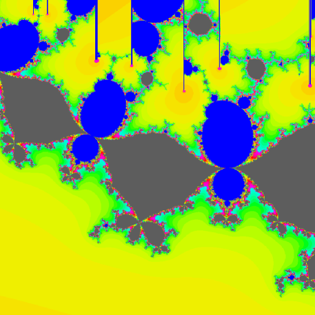
Figure 1: Part of the curve ${\mathcal{S}}_{4}$, represented in the $t$ parameter plane.

In principle, there is a great deal of choice involved here, since we can multiply $\Phi(z_{1},\,z_{2})$ by any function $\Psi(z_{1},\,z_{2})$ which is holomorphic and non-zero throughout a neighborhood of ${\mathcal{S}}$, and thus obtain many other local parametrizations. However, in the case of the period $p$ curve ${\mathcal{S}}_{p}$, there is one natural choice which seems convenient. Namely, using coordinates $(a,\,v)$ as above, we will work with the function

$$\Phi_{p}(a,\,v)~{}=~{}F^{\circ p}(a)-a$$

which by definition vanishes identically on ${\mathcal{S}}_{p}$, and which has no critical points near ${\mathcal{S}}_{p}$. (See [M, Theorem 5.2].)

Remark 2.1.

Although the canonical parameter $t$ is locally well defined up to translation in the $t$-plane, it does not follow that it can be defined globally. For example, computations show that there is a loop $L$ in ${\mathcal{S}}_{3}$ with

$$\int_{L}dt~{}\neq~{}0\,.$$

It follows that $t$ cannot be defined as a single valued function on ${\mathcal{S}}_{3}$. Conjecturally, the same is true for any ${\mathcal{S}}_{p}$ with $p\geq 3$.

3 Escape Regions and Associated Invariants.

By definition, an  escape region  ${\mathcal{E}}_{h}\subset{\cal S}_{p}$ is a connected component of the open subset of ${\mathcal{S}}_{p}$ consisting of maps $F\in{\mathcal{S}}_{p}$ for which the orbit of the free critical point  $-a$  escapes to infinity. This section will describe some basic invariants for escape regions in ${\mathcal{S}}_{p}$. The topology of ${\mathcal{E}}_{h}$ can be described as follows.

Lemma 3.1.

Each escape region ${\mathcal{E}}_{h}$ is canonically diffeomorphic to the $\mu_{h}$-fold covering of the complement ${\mathbb{C}}{\smallsetminus}\overline{\mathbb{D}}$, where $\mu_{h}\geq 1$ is an integer called the multiplicity of ${\mathcal{E}}_{h}$.

Figure 2: Sketch of the dynamic plane. Here ${\theta}\in{\mathbb{R}}/{\mathbb{Z}}$ is the co-critical angle.

Outline Proof. (For details, see [M, Lemma 5.9].) The dynamic plane for a map $~{}F\in{\mathcal{E}}_{h}$ is sketched in Figure 2.  The equipotential through the escaping critical point $-a=-a_{F}$ is a figure eight curve which also passes through the co-critical point $2a=2a_{F}$, and which completely encloses the filled Julia set $K(F)$. The Böttcher coordinate ${\mathfrak{B}}_{F}(z)\in{\mathbb{C}}{\smallsetminus}\overline{\mathbb{D}}$ is well defined for every $z$ outside of this figure eight curve, and is also well defined at the point $z=2a$. Setting $~{}{\mathfrak{B}}(F)\,=\,{\mathfrak{B}}_{F}(2a)$,  we obtain the required covering map

$$F~{}\mapsto~{}{\mathfrak{B}}(F)\,\in\,{\mathbb{C}}{\smallsetminus}\overline{\mathbb{D}}\;,$$

and define $~{}\mu_{h}\geq 1~{}$ to be the degree of this map. ∎

Definition 3.2.

Any smooth branch of the $~{}\mu$-th root function

$$F\mapsto\root{~{}\scriptstyle\mu} \of{{\mathfrak{B}}(F)}$$

yields a bijective map $~{}{\mathcal{E}}_{h}\stackrel{{\scriptstyle\cong}}{{\longrightarrow}}{\mathbb{C}}{\smallsetminus}\overline{\mathbb{D}}$.  Such a choice, unique up to multiplication by $~{}\mu$-th roots of unity, will be called an  anchoring of the escape region $~{}{\mathcal{E}}_{h}$.

Remark 3.3.

It is useful to compactify ${\mathcal{S}}_{p}$ by adjoining finitely many ideal points $\infty_{h}$, one for each escape region ${\mathcal{E}}_{h}$, thus obtaining a compact complex 1-manifold $\overline{\mathcal{S}}_{p}$. Thus each escape region, together with its ideal point, is conformally isomorphic to the open unit disk, with parameter $~{}1/\root\scriptstyle\mu \of{{\mathfrak{B}}(F)}$.

Although $t$ is a local uniformizing parameter near any finite point of ${\mathcal{S}}_{p}$, the $t$-plane is ramified over most ideal points. A typical picture of the $t$-plane for the curve ${\mathcal{S}}_{4}$ is shown in Figure 1. Here each ideal point in the figure is represented by a small red dot at the end of a slit in the $t$-plane. Each ideal point is surrounded by an escape region which has been colored yellow. The various escape regions are separated by the connectedness locus, which is colored blue for copies of the Mandelbrot set and brown for maps with only one attracting orbit.

Remark 3.4.

The number of escape regions, counted with multiplicity, is precisely equal to the degree of the curve ${\mathcal{S}}_{p}$. This grows exponentially with $p$. In fact, $~{}{\rm deg}({\mathcal{S}}_{p})~{}=~{}3^{p-1}+O(3^{p/2})~{}\sim~{}3^{p-1}~{}$ as $~{}p\to\infty$. (See [M, Remark 5.5].)

Remark 3.5.

The curve $~{}{\mathcal{S}}_{p}~{}$ has a canonical involution  ${\mathcal{I}}$ which sends the map $F:z\mapsto F(z)$ to the map ${\mathcal{I}}(F):z\mapsto-F(-z)$, rotating the Julia set by $180^{\circ}$, and also rotating parameter pictures in the canonical $t$-plane by $180^{\circ}$. In terms of the $(a,\,v)$ coordinates for $F$, it sends $\,(a,v)\,$ to $(-a,\,-v)$. This involution rotates some escape regions by $180^{\circ}$ around the ideal point, and matches other escape regions in disjoint pairs. (For tests to distinguish an escape region ${\mathcal{E}}_{h}$ from the  dual  region ${\mathcal{I}}({\mathcal{E}}_{h})$, see Remark 4.4.) We will also need the complex conjugation operation $~{}F_{a,\,v}\mapsto F_{\overline{a},\,\overline{v}}$,  or briefly $~{}F\mapsto\overline{F}\,$. (Compare §8.)

The Branner-Hubbard Puzzle, and the Associated Pseudometric, Marked Grid and Kneading Sequence.

Branner and Hubbard introduced the structure which is now called the Branner-Hubbard  puzzle ,  in order to study cubic polynomials which are outside of the connectedness locus. (See [BH], [Br].) They also introduced a diagram called the  marked grid  which captures many of the essential properties of the puzzle. In this subsection we first introduce a pseudometric that captures somewhat more of the basic properties of the puzzle. This pseudometric determines the associated marked grid. However, it does not distinguish between a region ${\mathcal{E}}_{h}$ and its complex conjugate region $\overline{\mathcal{E}}_{h}$ or its dual region ${\mathcal{I}}({\mathcal{E}}_{h})$.

For the moment, we do not need the hypothesis that $F\in{\mathcal{S}}_{p}$. However, we will assume that $F$ is monic and centered, that its marked critical orbit

$$a~{}=~{}a_{0}~{}\mapsto~{}a_{1}~{}\mapsto~{}a_{2}~{}\mapsto~{}\cdots$$

is bounded, and that the orbit of $-a_{0}$ is unbounded.

Definition 3.6.

The  puzzle piece $P_{0}$ of level zero  is defined to be the open topological disk consisting of all points $z$ in the dynamic plane such that

$$G_{F}(z)~{}<~{}G_{F}\big{(}F(-a)\big{)}~{}=3\,G_{F}(-a)\,,$$

where $G_{F}$ is the Green’s function (= potential function) which vanishes only on the filled Julia set $K_{F}$. For $\ell>0$, any connected component of the set

$$F^{-\ell}(P_{0})~{}=~{}\{z\in{\mathbb{C}}~{}~{};~{}~{}G_{F}(z)~{}<~{}G_{F}(-a)/3^{\ell-1}\}$$

is called a  puzzle piece of level $\ell$. The notation $P_{\ell}(z)$ will be used for the puzzle piece of level $\ell$ which contains some given point $z\in K_{F}$. Note that

$$P_{0}~{}=~{}P_{0}(z)~{}\supset~{}P_{1}(z)~{}\supset~{}P_{2}(z)~{}\supset~{}\cdots\,.$$

See Figure 2 for a schematic picture of the puzzle pieces of levels zero and one.

Definition 3.7.

Given two points $x$ and $y$ in $K_{F}$, define the  greatest common level  $L(x,y)\in{\mathbb{N}}\cup\infty$ to be the largest integer $\ell$ such that

$$P_{\ell}(x)~{}=~{}P_{\ell}(y)\,,$$

setting $~{}L(x,y)=\infty~{}$ if $~{}P_{\ell}(x)=P_{\ell}(y)~{}$ for all levels $\ell$. The  puzzle pseudometric  on the filled Julia set $K_{F}$ is defined by the formula

$$d_{F}(x,\,y)~{}=~{}2^{-L(x,y)}~{}\in~{}[0,\,1]\,.$$

Thus

$$d_{F}(x,\,y)~{}=~{}\begin{cases}0\qquad\qquad\quad{\rm whenever}\quad P_{\ell}(x)~{}=~{}P_{\ell}(y)\quad{\rm for~{}every~{}level}~{}~{}\ell\,,\\ 2^{-\ell}\,>\,0\qquad{\rm if}~{}~{}\ell\geq 0~{}~{}{\rm is~{}the~{}largest~{}integer~{}with}~{}~{}P_{\ell}(x)\,=\,P_{\ell}(y)\,.\end{cases}$$

Since the special case $x=a_{0}$ will play a particularly important role, we sometimes use the abbreviations

$$L_{0}(y)~{}=L(a_{0},\,y)\qquad{\rm and}\qquad d_{0}(y)~{}=~{}d_{F}(a_{0},\,y)\,.$$ (1)

The basic properties of this pseudometric can be described as follows.

Lemma 3.8.

For all $~{}x,\,y,\,z\in K_{F}$,  we have:

• Ultrametric inequality. $~{}~{}~{}~{}d_{F}(x,z)\,\leq\,\max\big{(}d_{F}(x,y),\;d_{F}(y,z)\big{)}$, with equality whenever $d_{F}(x,y)\neq d_{F}(y,z)$.

• $d_{F}(x,y)\,d_{F}(x,z)\,d_{F}(y,z)~{}<~{}1\,.$

• $d_{F}\big{(}F(x),\,F(y)\big{)}~{}\leq~{}2\,d_{F}(x,\,y)\,,$  and furthermore

• if  $d_{F}\big{(}F(x),\,F(y)\big{)}\,<\,2\,d_{F}(x,\,y)$    with   $d_{F}(x,y)<1$,  then

  $$d_{F}(x,y)~{}=~{}d_{0}(x)~{}=~{}d_{0}(y)~{}>~{}0\,.$$

• $d_{F}(x,y)~{}=~{}0$  if and only if $x$ and $y$ belong to the same connected component of $K_{F}$.

As an example, applying (c) and (d) to the case $x=a_{0}$, it follows immediately that

$$d\big{(}a_{1},\,F(y)\big{)}\,=\,2\,d_{F}(a_{0},\,y)\quad{\rm whenever}\quad d_{F}(a_{0},\,y)<1\,.$$ (2)

Proof of Lemma 3.8. Assertion (a) follows immediately from the definition, and (b) is true because there are only two puzzle pieces of level one. The proof of (c) and (d) will be based on the following observation.

Call a puzzle piece  critical  if it contains the critical point $a_{0}$, and  non-critical  otherwise. Then $F$ maps each puzzle piece $P_{\ell}(x)$ of level $\ell>0$ onto the puzzle piece $P_{\ell-1}\big{(}F(x)\big{)}$ by a map which is a two-fold branched covering if $P_{\ell}(x)$ is critical, but is a diffeomorphism if $P_{\ell}(x)$ is non-critical. If $x$ and $y$ are contained in a common piece of level $\ell>0$, then it follows that $F(x)$ and $F(y)$ are contained in a common piece of level $\ell-1$; which proves (c). Now suppose that $d_{F}(x,y)=2^{-\ell}<1$, and that $d\big{(}F(x),\,F(y)\big{)}\leq 2^{-\ell}$. Then the two distinct puzzle pieces $P_{\ell+1}(x)$ and $P_{\ell+1}(y)$, both contained in $P_{\ell}(x)$, must map onto a common puzzle piece $P_{\ell}\big{(}F(x)\big{)}$. Clearly this can happen only if $P_{\ell}(x)$ also contains the critical point $a_{0}$, but neither $P_{\ell+1}(x)$ nor $P_{\ell+1}(y)$ contains $a_{0}$. Thus we must have $d_{F}(x,y)=d_{F}(a_{0},x)=d_{F}(a_{0},y)$, which proves (d). For the proof of (e), see [BH, §5.1]. ∎

A fundamental result of the Branner-Hubbard theory can be stated as follows, using this pseudometric terminology.

Theorem 3.9.

Let $K_{0}\subset K_{F}$ be the connected component of the filled Julia set which contains the critical point $a_{0}$. Suppose that $d_{F}(a_{0},\,a_{n})=0$ for some integer $n\geq 1$. $($In other words, suppose that $P_{\ell}(a_{0})=P_{\ell}(a_{n})$ for all levels $\ell\,.)$  If $n$ is minimal, then $F^{\circ n}$ restricted to some neighborhood of $K_{0}$ is polynomial-like, and is hybrid equivalent to a uniquely defined quadratic polynomial $Q$ with connected Julia set. In this case, countably many connected components of $K_{F}$ are homeomorphic copies of $K_{Q}$, and all other components are points.

Proof. See Theorems 5.2 and 5.3 of [BH]. (In their terminology, the hypothesis that $d_{F}(a_{0},\,a_{n})=0$ is expressed by saying that the  marked grid  of the critical orbit has period $n$. Compare Definition 3.12 below.) ∎

By definition, $Q$ will be called the  associated quadratic map. If $F$ belongs to the period $p$ curve ${\mathcal{S}}_{p}$, then evidently the hypothesis of Theorem 3.9 is always satisfied, for some smallest integer $n\geq 1$ which necessarily divides $p$. It then follows that the critical point $a_{0}$ has period $p/n$ under the map $F^{\circ n}$. Thus we obtain the following.

Corollary 3.10.

If $F\in{\mathcal{S}}_{p}$ satisfies the hypothesis of Theorem 3.9, then the associated quadratic map $Q$ is critically periodic of period $p/n$.

Remark 3.11 (Erratum to [M]).

Unfortunately, an incorrect version of Corollary 3.10 was stated in [M, Theorem 5.15], based on the erroneous belief than every escape region with kneading sequence of period $n$ must also have a marked grid of period $n$. (See Definitions 3.12 and 3.14 below.) For counterexamples, see Example 3.16.

The marked grid associated with an orbit $z_{0}\mapsto z_{1}\mapsto\cdots$ in $K_{F}$ is a graphic method of visualizing the sequence of numbers

$$L_{0}(z_{0}),~{}L_{0}(z_{1}),~{}L_{0}(z_{2}),~{}\ldots~{}\in~{}{\mathbb{N}}\cup\infty~{},$$

which describe the extent to which this orbit approaches the marked critical point $a_{0}$. The marked grid for the critical orbit $a_{0}\mapsto a_{1}\mapsto a_{2}\mapsto\cdots$ plays a particularly important role in the Branner-Hubbard theory, and is the only grid that we will consider.

Definition 3.12.

The critical marked grid $M=[M(\ell,\,k)]$, associated with the critical orbit $a_{0}\mapsto a_{1}\mapsto\cdots$ in $K_{F}$, can be described as an infinite matrix of zeros and ones, indexed by pairs $(\ell,\,k)$ of non-negative integers. By definition, $M(\ell,\,k)=1$ if and only if $\ell\leq L_{0}(a_{k})$; that is, if and only if the puzzle piece $P_{\ell}(a_{k})$ is critical, that is, if and only if

$$P_{\ell}(a_{0})~{}=~{}P_{\ell}(a_{k})\qquad\Longleftrightarrow\qquad d_{F}(a_{0},\,a_{k})~{}\leq~{}2^{-\ell}\,.$$

Grid points $(\ell,\,k)$ with $M(\ell,\,k)=1$ are said to be marked. This matrix is represented graphically by an infinite tree where the marked points $(\ell,\,k)$ are represented by heavy dots joined vertically, and joined horizontally along the entire top line $\ell=0$. This marked grid remains constant throughout the escape region.

Figure 3: Marked grid for the critical orbit of a map belonging to any one of four different escape regions in ${\mathcal{S}}_{4}$. For each $k\geq 0$, there are $L_{0}(a_{k})$ vertical edges in the $k$-th column.

Figure 4: Schematic picture illustrating the puzzle pieces of level one and two for the two possible types of map in ${\mathcal{S}}_{4}$ with kneading sequence $\overline{1000}$. In both cases, the equipotentials through $-a$ and through $F^{-1}(-a)$ are shown. Each point $~{}a_{j}=F^{\circ j}(a)~{}$ of the critical orbit is labeled briefly as $~{}j$.  Thus the points $a_{2}$ and $a_{3}$ are separated in the $\overline{\rm 1000}$s case, but are together in the $\overline{\rm 1000}$t case.

As an example, Figure 3 shows one of the possible critical grids of period 4 for maps belonging to an escape region in $~{}{\mathcal{S}}_{4}$.  In fact, there are four disjoint escape regions which give rise to this same marked grid. However, up to isomorphism there are only two distinct types, since the $180^{\circ}$ rotation $~{}{\mathcal{I}}~{}$ of Remark 3.5 carries each of these regions to a disjoint but isomorphic region. See Figure 4, which sketches levels one and two of the puzzles corresponding to the two distinct types. (Compare Example 3.15.)

Since the critical orbit has period 4, the associated pseudometric on the critical orbit is completely described by the symmetric $4\times 4$ matrix of distances $[d_{F}(a_{i},\,a_{j})]$,  with $0\leq i,\,j<4$. The matrices corresponding to these two puzzles are given by

$$\left[\begin{matrix}0&1&1/2&1/2\\ 1&0&1&1\\ 1/2&1&0&1/2\\ 1/2&1&1/2&0\end{matrix}\right]\qquad{\rm and}\qquad\left[\begin{matrix}0&1&1/2&1/2\\ 1&0&1&1\\ 1/2&1&0&1/4\\ 1/2&1&1/4&0\end{matrix}\right]$$

respectively. Thus $d_{F}(a_{2},\,a_{3})$ is equal to $1/2$ in one case and $1/4$ in the other. However the marked grid, which is a graphic representation of the top row of the matrix, is the same for these two cases.

Every such critical marked grid must satisfy three basic rules, as stated in [BH], and also a fourth rule as stated in [K1].

Theorem 3.13.

(The Four Grid Rules)

• $1\,=\,M(0,\,k)~{}\geq~{}M(1,\,k))~{}\geq~{}M(2,\,k)~{}\geq~{}\cdots~{}\geq~{}0\,.$

• If $M(\ell,\,k)=1$, then $M(\ell-i,\,k+i)=M(\ell-i,\,i)$ for $0\leq i\leq\ell$.

• Suppose that $d_{F}(a_{0},\,a_{m})=2^{-\ell}$, that $d_{F}(a_{0},\,a_{i})>2^{i-\ell}$ for $0<i<k$ and that $~{}d_{F}(a_{0},\,a_{k})<2^{k-\ell}$. Then $~{}d_{F}(a_{0},\,a_{m+k})=2^{k-\ell}$.

• Suppose that $d_{F}(a_{0},\,a_{k})=2^{-\ell}$, that $d_{F}(a_{0},\,a_{k+i})>2^{i-\ell}$ for $0<i<\ell$, and that $~{}d_{F}(a_{0},\,a_{\ell})=1$. Then $~{}d_{F}(a_{0},\,a_{\ell+k})<1$.

Proof. All four rules are consequences of Lemma 3.8.

R1: The First Rule follows immediately from Definition 3.7.

R2: For the Second Rule, the statement $M(\ell,\,k)=1$ means that

$$~{}d_{F}(a_{0},\,a_{k})~{}\leq~{}2^{-\ell}~{}.$$

It then follows inductively, using Lemma 3.8-(c), that $d_{F}(a_{i},\,a_{k+i})\leq 2^{i-\ell}$. The ultrametric inequality then implies that

$$d_{F}(a_{0},\,a_{i})~{}\leq~{}2^{i-\ell}~{}\qquad\Longleftrightarrow\qquad d_{F}(a_{0},\,a_{k+i})~{}\leq~{}2^{i-\ell}\,,$$

which is equivalent to the required statement.

R3: To prove the Third Rule, we will first show by induction on $i$ that

$$d_{F}(a_{i},\,a_{m+i})~{}=~{}2^{i}\,d_{F}(a_{0},\,a_{m})~{}=~{}2^{i-\ell}$$

for $0\leq i\leq k$. The assertion is certainly true for $i=0$. If it is true for $i$, then it follows for $i+1$ by Lemma 3.8 items (c) and (d), unless

$$d_{F}(a_{i},\,a_{m+i})~{}=~{}d_{F}(a_{0},\,a_{i})~{}=~{}d_{F}(a_{0},\,a_{m+i})\,.$$

This last equation is impossible since $d_{F}(a_{i},\,a_{m+i})=2^{i-\ell}$ by the induction hypothesis but $d_{F}(a_{0},\,a_{i})>2^{i-\ell}$. In particular, it follows that $d_{F}(a_{k},\,a_{m+k})~{}=~{}2^{k-\ell}$. Since $d_{F}(a_{0},\,a_{k})<2^{k-\ell}$, the required equation $d_{F}(a_{0},\,a_{m+k})~{}=~{}2^{k-\ell}$  follows by the ultrametric inequality.

R4: Since $d_{F}(a_{0},\,a_{k})=2^{-\ell}$, it follows inductively that $d_{F}(a_{i},a_{i+k})=2^{i-\ell}$ for $i\leq\ell$. For otherwise by Lemma 3.8 items (c) and (d), we would have to have

$$d_{F}(a_{0},\,a_{i})~{}=~{}d_{F}(a_{0},\,a_{i+k})~{}=~{}d_{F}(a_{i},\,a_{i+k})$$

for some $i<\ell$, which contradicts the hypothesis. In particular, this proves that $d_{F}(a_{\ell},\,a_{\ell+k})=1$. Since $d_{F}(a_{0},\,a_{\ell})=1$, it follows from Lemma 3.8-(b) that $d_{F}(a_{0},\,a_{\ell+k})<1$, as asserted.$\quad\square$

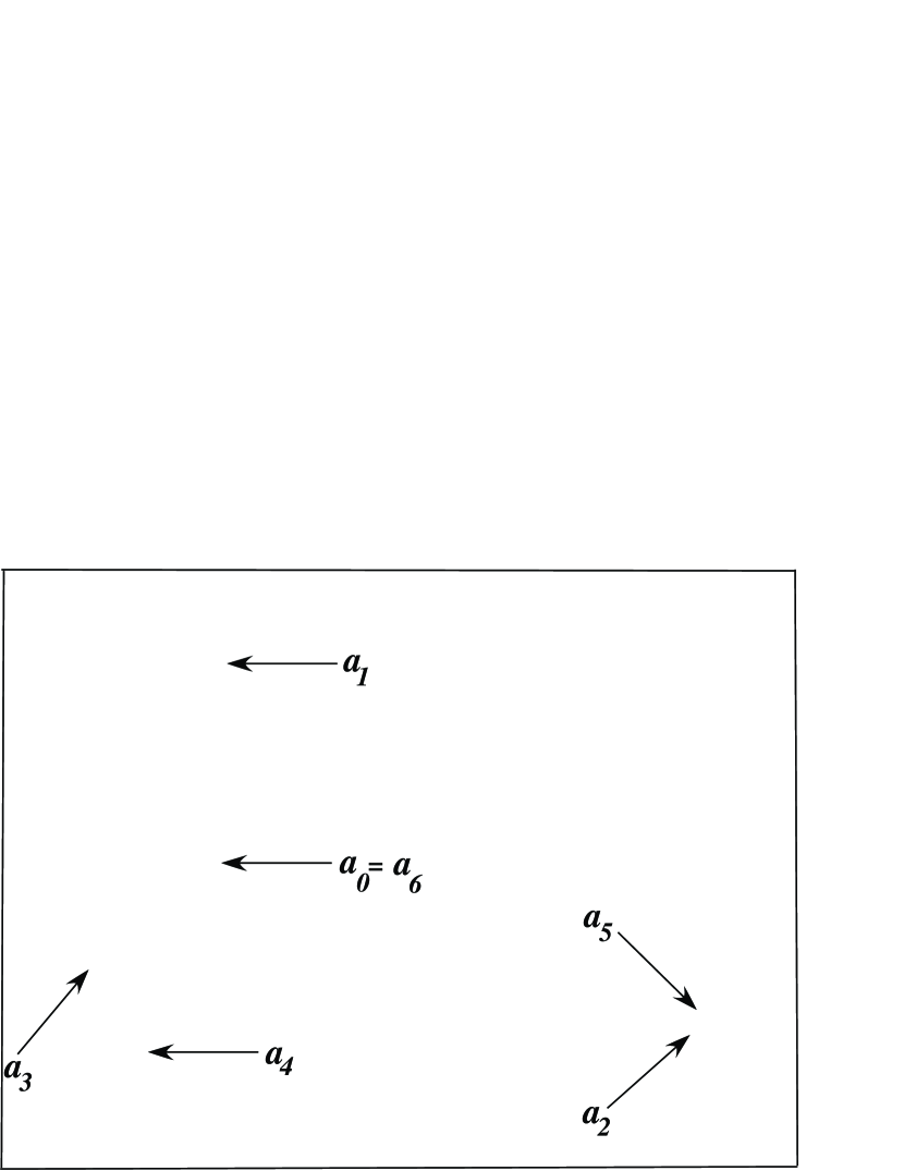
Figure 5: Julia set of a polynomial map in $~{}{\mathcal{S}}_{6}$ with marked grid of period $6$ but kneading sequence $\overline{010010}$ of period $3$, showing the puzzle pieces of level one, two and three.

For some purposes, it is convenient to work with an even weaker invariant. (Compare [M, §5B].)

Definition 3.14.

The  kneading sequence  of an orbit $z_{0}\mapsto z_{1}\mapsto\cdots$ in $K_{F}$ is the sequence

$$\sigma(z_{0}),\,\sigma(z_{1}),\,\sigma(z_{2}),\,\cdots$$

of zeros and ones, where

$$\sigma(z_{j})~{}=~{}\begin{cases}0\qquad{\rm if}~{}~{}d_{F}(z_{j},\,a_{0})<1~{},\\ 1\qquad{\rm if}~{}~{}d_{F}(z_{j},\,a_{0})=1~{}.\end{cases}$$

In other words, $~{}\sigma(z_{j})=0~{}$ if $z_{j}$ and $a_{0}$ belong to the same puzzle piece of level one, but $~{}\sigma(z_{j})=1~{}$ if they belong to different puzzle pieces of level one.

As an immediate application of the inequalities (b) and (c) of Lemma 3.8, we have the following.

$${\rm If}~{}\sigma_{j+n}(z_{0})\neq\sigma_{k+n}(z_{0})~{}~{}{\rm for~{}some}~{}~{}n\geq 0\,,~{}{\rm then}~{}~{}d_{F}(z_{j},\,z_{k})\geq 2^{-n}>0\,.$$

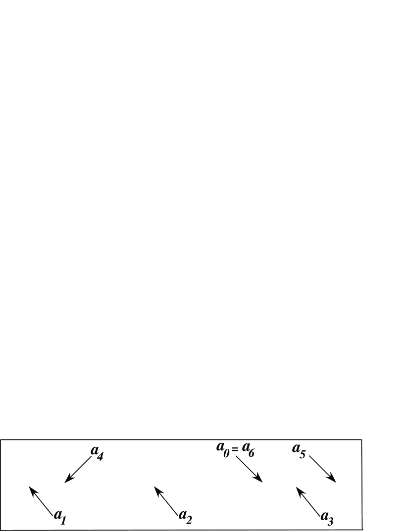
Figure 6: A real example in ${\mathcal{S}}_{6}$ with kneading sequence $\overline{100100}$ of period $3$ and marked grid of period $6$. The Julia set and puzzle structure are shown above, and the graph of $F:{\mathbb{R}}\to{\mathbb{R}}$ below. $($Similarly, Figure $5$ could be replaced by a pure imaginary example, with $~{}a,\,v\in i\,{\mathbb{R}}\,.)$

Again we are principally interested in the critical orbit $a_{0}\mapsto a_{1}\mapsto\cdots$. The knowledge of the critical kneading sequence is completely equivalent to the knowledge of the level one row of the critical marked grid; in fact

$$\sigma(a_{j})~{}=~{}1-M(1,j)\,.$$

The notation

$$\stackrel{{\scriptstyle\to}}{{\sigma}}~{}=~{}(~{}\sigma(a_{1}),\,\sigma(a_{2}),\,\sigma(a_{3}),\,\ldots~{})$$

will be used for the kneading sequence of the critical orbit (omitting the initial $\sigma(a_{0})$ since it is always zero by definition). In the period $p$ case, we will also write this as

$$\stackrel{{\scriptstyle\to}}{{\sigma}}~{}=~{}\overline{\sigma_{1}\sigma_{2}\cdots\sigma_{p-1}0}\,,$$

where the overline refers to infinite repetition; or informally just refer to the periodic sequence $\sigma_{1}\sigma_{2}\cdots\sigma_{p-1}0$. With this notation, note that the final bit must always be zero.

Example 3.15.

For periods $~{}p~{}\leq~{}3$,  the kneading invariant together with the associated quadratic map suffices to characterize the escape region, up to canonical involution. However, for escape regions in $~{}{\mathcal{S}}_{4}~{}$ with kneading sequence $~{}\overline{1000}$,  a “secondary kneading invariant” is needed to specify whether the second and third forward images of $~{}a~{}$ are “separate” or “together.” (See Figure 4.) For higher periods, many more such distinctions are necessary. (Compare Example 5.6.)

Example 3.16.

Figures 5 and 6 show examples of maps in ${\mathcal{S}}_{6}$ which have kneading sequence of period 3 but marked grid of period 6. (Parameter values for Figure 5: $~{}a\,=\,-0.8004\,+\,0.2110\,i\,,\quad v\,=\,-0.77457275\,+\,1.24396437\,i$,Figure 6: $~{}a\,=\,1.028778\,,\quad v\,=\,-1.877412$.)   The corresponding marked grids are shown in Figure 7.

    

Figure 7: Marked grids corresponding to Figures 5 and 6.

4 Puiseux Series.

(Compare [K1].) Recall from Lemma 3.1 that for each escape region ${\mathcal{E}}_{h}\subset{\mathcal{S}}_{p}$ the projection map $(a,v)\mapsto a$ from ${\mathcal{E}}_{h}$ to the complex numbers has a pole of order $\mu\geq 1$ at the ideal point $\infty_{h}$. It will be more convenient to work with the variable

$$\xi~{}=~{}1/(3a)$$

which is a bounded holomorphic function throughout a neighborhood of $\infty_{h}$ in ${\mathcal{S}}_{p}$. (The factor 3 has been inserted here in order to simplify later formulas.) Since $\xi$ has a zero of order $\mu$, we can choose some $\mu$-th root $~{}\xi^{1/\mu}~{}$ as a local uniformizing parameter near the ideal point.

Remark 4.1.

This choice of local parameter $~{}\xi^{1/\mu}~{}$ is completely equivalent to the choice of anchoring $~{}{\mathfrak{B}}(F)^{1/\mu}$  in Definition 3.2. In fact, the function $~{}F_{a,v}\mapsto{\mathfrak{B}}(F_{a,v})\,=\,{\mathfrak{B}}_{F_{a,v}}(2\,a)~{}$ is asymptotic to $~{}2\,a=2/(3\,\xi)$  as $~{}|a|\to\infty$,  so that the product $~{}\xi\,\,{\mathfrak{B}}(F)$  converges to $~{}2/3\,$. Hence we can always choose the $~{}\mu$-th roots so that their product converges to the positive root $~{}(2/3)^{1/\mu}>0$.

Let

$$a_{0}\mapsto a_{1}\mapsto a_{2}\mapsto\cdots\mapsto a_{p}=a_{0}$$

be the periodic critical orbit, with $a=a_{0}$ and $F(a)=v=a_{1}$. Then each $a_{j}$ can be expressed as a meromorphic function of $~{}\xi^{1/\mu}~{}$, with a pole at the ideal point. More precisely, according to [M, Theorem 5.16], each $a_{j}$ can be expressed as a meromorphic function of the form

$$a_{j}=\begin{cases}\quad a+O(1)\qquad{\rm if}\quad\sigma_{j}=0~{},\cr-2a+O(1)\quad\;\;{\rm if}\quad\sigma_{j}=1\end{cases}$$

where each $O(1)$ term represents a holomorphic function of $~{}\xi^{1/\mu}~{}$ which is bounded for small $|\xi|$. (Compare Lemma 4.3 below.) In order to replace the $a_{j}$ by holomorphic functions, we introduce the new variables

$$u_{j}~{}=~{}\frac{a-a_{j}}{3\,a}\,.$$ (3)

Evidently each $u_{j}$ is a globally defined meromorphic function on ${\mathcal{S}}_{p}$. Within a neighborhood of the ideal point $\infty_{h}$, each $u_{j}$ is a bounded holomorphic function of the local uniformizing parameter $~{}\xi^{1/\mu}~{}$. In fact, this particular expression (3) has been chosen so that $u_{j}$ takes the convenient value

$$u_{j}(0)~{}=~{}\sigma_{j}~{}\in~{}\{0,\,1\}$$

at the ideal point $\xi=0$. More precisely, each $u_{j}$ has a power series of the form

$$u_{j}~{}=~{}\sigma_{j}~{}+~{}a_{\mu}\xi~{}+~{}a_{\mu+1}\xi^{1+1/\mu}~{}+~{}a_{\mu+2}\xi^{1+2/\mu}~{}+~{}\cdots$$ (4)

which converges for small $~{}|\xi|$,  with $\sigma_{j}$ as in Definition 3.14. We will refer to this as the  Puiseux expansion  of $u_{j}$, since it is a power series in fractional powers of $\xi$.

Note that $u_{0}=u_{p}=0$ by definition. Recall the equation

$$a_{j+1}~{}=~{}F(a_{j})~{}=~{}a_{j}^{3}-3a^{2}a_{j}+2a^{3}+v~{}=~{}(a_{j}-a)^{2}(a_{j}+2a)+a_{1}\,.$$

Substituting $a_{j}=a(1-3u_{j})=a-u_{j}/\xi$, this reduces easily to the following equations, which will play a fundamental role.

$$\xi^{2}(u_{j+1}-u_{1})~{}=~{}u_{j}^{\,2}(u_{j}-1)\,,\qquad{\rm or}\qquad u_{j+1}~{}=~{}u_{1}+u_{j}^{\,2}(u_{j}-1)/\xi^{2}\,.$$ (5)

Thus, if we are given the Puiseux series for $u_{1}=(a-v)/3a$, then the series for $u_{2},\,u_{3},\,\ldots,\,u_{p}$ can easily be computed inductively.

Example 4.2 (Escape Regions in ${\mathcal{S}}_{2}$).

Consider the case $p=2$. Since $u_{2}=0$, there is just one unknown function $u_{1}$, which must satisfy Equation (5), that is $~{}0=u_{1}+u_{1}^{\,2}(u_{1}-1)/\xi^{2}$,  or in other words

$$u_{1}^{\,3}~{}-~{}u_{1}^{\,2}~{}+~{}\xi^{2}u_{1}~{}=~{}0\,.$$

This cubic equation in $u_{1}$ has three solutions, namely $u_{1}=0$ corresponding to the unique escape region in ${\mathcal{S}}_{1}$, and the two solutions

$$u_{1}~{}=~{}\textstyle{\frac{1}{2}}\Big{(}1\pm\sqrt{1-4\xi^{2}}\Big{)}~{}=~{}\textstyle{\frac{1}{2}}\Big{(}1\pm(1-2\xi^{2}-2\xi^{4}-4\xi^{6}-\cdots)\Big{)}$$

or in other words

$$u_{1}~{}=~{}\begin{cases}1-\xi^{2}-\xi^{4}-2\xi^{6}-\cdots\,\quad&{\rm if\;the\;kneading\;sequence\;is~{}\;}\overline{10}\,,\cr 0+\xi^{2}+\xi^{4}+2\xi^{6}+\cdots\,\quad&{\rm if\;it\;is~{}\;}\overline{00}\,,\end{cases}$$ (6)

corresponding to the two escape regions in ${\mathcal{S}}_{2}$.

Using the Equations (5), it is not difficult to obtain asymptotic estimates.

Lemma 4.3.

For $~{}F\in{\mathcal{E}}_{h}\subset{\mathcal{S}}_{p}~{}$ and for $~{}0<j<p$,  we have the following asymptotic estimates as $~{}\xi\to 0~{}$ or as $~{}|a|\to\infty$.

$$u_{j}~{} \sim ~{}\pm\xi\sqrt{u_{1}-u_{j+1}}\,\qquad{\rm if}\qquad\sigma_{j}=0\,,$$ (7)

$$u_{j}-1~{} \sim ~{}~{}\xi^{2}(u_{j+1}-u_{1})\quad\qquad{\rm if}\qquad\sigma_{j}=1\,.$$ (8)

Given only the kneading sequence $~{}\stackrel{{\scriptstyle\to}}{{\sigma}}$, we can state these estimates as follows.

$$u_{j}~{} = ~{}\pm\xi\sqrt{\sigma_{1}-\sigma_{j+1}}~{}+~{}O(\xi^{3/2})\quad\qquad{\rm if}\quad\sigma_{j}=0\,,$$ (9)

$$u_{j}~{} = ~{}1~{}+~{}\xi^{2}(\sigma_{j+1}-\sigma_{1})~{}+~{}O(\xi^{3})\qquad\;{\rm if}\quad\sigma_{j}=1\,.$$ (10)

(In special cases, it is often possible to improve these error estimates.) The proofs are easily supplied. ∎

Remark 4.4.

As an example, still assuming that $~{}0<j<p$,  it follows that $~{}u_{j}~{}$ has the form

$$u_{j}~{}=~{}\beta\,\xi~{}+~{}{\rm(higher~{}order~{}terms)}\qquad{\rm with}\qquad\beta\neq 0$$ (11)

if and only if $~{}\sigma_{j}=0$  and $~{}\sigma_{j+1}\neq\sigma_{1}$. Here

$$\beta~{}=~{}\pm 1\qquad{\rm when}\qquad\sigma_{1}-\sigma_{j+1}~{}=~{}+1\,,$$

but

$$\beta~{}=~{}\pm i\qquad{\rm when}\qquad\sigma_{1}-\sigma_{j+1}~{}=~{}-1\,.$$

In both cases, the equation $~{}a_{0}-a_{j}=u_{j}/\xi$,  implies that we have the following limiting formula as $~{}\xi\to 0~{}$ (or as $~{}|a|\to\infty\,$):

$$\lim_{\xi\to 0}~{}(a_{j}~{}-~{}a_{0})~{}=~{}\beta~{}\neq~{}0\,.$$

It follows that ${\mathcal{E}}_{h}\neq{\mathcal{I}}({\mathcal{E}}_{h})$, since the difference $a_{j}-a_{0}$ changes sign when we replace the region ${\mathcal{E}}_{h}$ by its dual ${\mathcal{I}}({\mathcal{E}}_{h})$. Still assuming (11), the approximate equality

$$a_{0}~{}-a_{j}~{}\approx~{}\beta\,,$$

holds for all maps $~{}F\in{\mathcal{E}}_{h}~{}$ with $~{}|a_{0}|~{}$ large. As an example, Figure 5 illustrates a case with $a_{1}\approx a_{0}+i$. In fact, assuming (11), we can usually distinguish between maps in the regions ${\mathcal{E}}_{h}$ and ${\mathcal{I}}({\mathcal{E}}_{h})$ simply by checking the sign of the real part $~{}\Re\big{(}(a_{0}-a_{j})/\beta\big{)}$.

Remark 4.5.

Recall that $u_{p}=0$ by definition. The requirement that $u_{p}=0$, together with the set of Equations (5), imposes a very strong restriction as to which series $u_{1}$ can occur. In fact this is the only restriction. A priori, there could be formal power series solutions to the Equations (5) with $u_{p}=0$ which have zero radius of convergence, and hence do not correspond to any actual escape region. However, every such solution satisfies a polynomial equation of degree $3^{p-1}$ in the field of formal Puiseux series, and a counting argument shows that every solution corresponds to an actual escape region in some ${\mathcal{S}}_{n}$, where $n$ must divide $p$. In particular, every solution has a positive radius of convergence, and the corresponding functions

$$a~{}=~{}1/\,3\,\xi\,,\qquad v~{}=~{}\big{(}1-3u_{1}(\xi^{1/\mu})\big{)}/3\,\xi$$

parameterize a neighborhood of the ideal point in a corresponding escape region.

Remark 4.6.

In the case of an escape region of multiplicity $\mu>1$, some comment is needed. There are $\mu$ possible choices for a preferred $\mu$-th root of the holomorphic function $\xi$, and these will give rise to $\mu$ different power series for the function $u_{1}$. We can think of these various solutions as elements of the field ${\mathbb{C}}(({\boldsymbol{\xi}}^{1/\mu}))$ of formal power series. (The bold ${\boldsymbol{\xi}}$ symbol is used to emphasize that we are now thinking of ${\boldsymbol{\xi}}$ as a formal indeterminate rather than a complex variable.) However these different series for the same escape region are all conjugate to each other under a Galois automorphism ${\boldsymbol{\xi}}^{1/\mu}\mapsto\alpha{\boldsymbol{\xi}}^{1/\mu}$ from ${\mathbb{C}}(({\boldsymbol{\xi}}^{1/\mu}))$ to itself which fixes every point of the sub-field ${\mathbb{C}}(({\boldsymbol{\xi}}))$. Here $\alpha$ is to be an arbitrary $\mu$-th root of unity. Thus we have outlined a proof of the following.

Theorem 4.7.

There is a one-to-one correspondence between escape regions in ${\mathcal{S}}_{p}$ and Galois conjugacy classes of solutions to the set of Equations $(\ref{e-u-condition})$ with $u_{p}=0$, where $p$ is minimal.

5 The Leading Monomial.

Clearly it is enough to specify finitely many terms of the Puiseux series $u_{1},\,\ldots,$ $u_{p-1}$ in order to determine all of the $u_{j}$ uniquely, and hence determine the corresponding escape region uniquely. In fact, it turns out that it is always enough to know just the leading term of each $u_{j}$. (Equivalently, it is enough to known the asymptotic behavior of each difference $a_{j}-a_{0}$ as $|a|=|a_{0}|$ tends to infinity. Compare Remark 4.4.)

It will be convenient to work with formal power series. Let

$${\mathbf{u}}_{j}~{}=~{}{\mathbf{u}}_{j}({\boldsymbol{\xi}}^{1/\mu})~{}\in~{}{\mathbb{C}}[[{\boldsymbol{\xi}}^{1/\mu}]]$$

be the formal power series expansion for the holomorphic function $u_{j}=u_{j}(\xi^{1/\mu})$. If a power series $~{}{\mathbf{x}}\in{\mathbb{C}}[[{\boldsymbol{\xi}}^{1/\mu}]]~{}$ has the form

$${\mathbf{x}}~{}=~{}\beta\,{\boldsymbol{\xi}}^{q}~{}+~{}({\rm higher~{}order~{}terms})\qquad{\rm with}\qquad\beta\neq 0\,,$$

then the monomial $~{}{\mathbf{m}}=\beta\,{\boldsymbol{\xi}}^{q}~{}$ is called the  leading term  of $~{}{\mathbf{x}}$,  and the rational number $~{}q~{}$ is called the order,

$${\rm ord}({\mathbf{x}})~{}=~{}{\rm ord}({\mathbf{m}})~{}=~{}q\,.$$

For the special case $~{}{\mathbf{x}}={\bf 0}\,$, the order is defined to be $~{}{\rm ord}({\bf 0})=+\infty$.

Closely related is the  formal power series metric, associated with the norm

$$\|{\mathbf{x}}\|~{}=~{}e^{-{\rm ord}({\mathbf{x}})}\,.$$ (12)

This satisfies the  ultrametric inequality

$$\|{\mathbf{x}}\pm{\mathbf{y}}\|~{}\leq~{}{\rm max}(\|{\mathbf{x}}\|,\,\|{\mathbf{y}}\|)\,.$$ (13)

Two formal power series are  asymptotically equal,  ${\mathbf{x}}~{}\sim~{}{\mathbf{x}}^{\prime}$, if they have the same leading term. We will also use the $O({\boldsymbol{\xi}}^{q})$ and $o({\boldsymbol{\xi}}^{q})$ notations, defined as follows in the formal power series context:

$$\begin{matrix}{\mathbf{x}}=O({\boldsymbol{\xi}}^{q})&\Longleftrightarrow&{\mathbf{x}}~{}\equiv 0~{}~{}~{}~{}({\rm mod}~{}{\boldsymbol{\xi}}^{q})&\Longleftrightarrow&{\rm ord}({\mathbf{x}})\geq q\,,&{\rm and}\\ {\mathbf{x}}=o({\boldsymbol{\xi}}^{q})&\Longleftrightarrow&{\mathbf{x}}~{}\equiv 0~{}~{}({\rm mod}~{}{\boldsymbol{\xi}}^{q+1/\mu})&\Longleftrightarrow&{\rm ord}({\mathbf{x}})>q\,.&\end{matrix}$$

It will be convenient to use notations such as $~{}\stackrel{{\scriptstyle\to}}{{{\mathbf{w}}}}~{}$ for a $p$-tuple$~{}({\mathbf{w}}_{1},\ldots,\,{\mathbf{w}}_{p-1}\,,0)$  with ${\mathbf{w}}_{p}=0$,  and to define the “error” $E_{j}=E_{j}(\stackrel{{\scriptstyle\to}}{{{\mathbf{w}}}})$ by the formula

$$E_{j}(\stackrel{{\scriptstyle\to}}{{{\mathbf{w}}}})~{}=~{}{\boldsymbol{\xi}}^{2}({\mathbf{w}}_{j+1}-{\mathbf{w}}_{1})\;-\;{\mathbf{w}}_{j}^{\,2}({\mathbf{w}}_{j}-1)\,$$ (14)

for $~{}0<j<p$. Thus the required Equation (5) can be written briefly as $~{}~{}E_{j}(\stackrel{{\scriptstyle\to}}{{{\mathbf{u}}}})~{}=~{}0\,.$

Theorem 5.1 (Kiwi).

For any escape region $~{}{\mathcal{E}}_{h}\subset{\mathcal{S}}_{p}$,  the vector

$$~{}\stackrel{{\scriptstyle\to}}{{{\mathbf{u}}}}~{}=~{}({\mathbf{u}}_{1},\,{\mathbf{u}}_{2},\,\ldots,\,{\mathbf{u}}_{p-1},\,{\boldsymbol{0}})~{}$$

of Puiseux series is uniquely determined by the associated vector

$$~{}\stackrel{{\scriptstyle\to}}{{{\mathbf{m}}}}~{}=~{}({\mathbf{m}}_{1},\,{\mathbf{m}}_{2},\,\ldots,\,{\mathbf{m}}_{p-1},\,{\boldsymbol{0}})~{}$$

of leading monomials.

The proof will appear in [K2] .∎

Evidently these leading monomials $~{}{\mathbf{m}}_{j}~{}$ determine and are determined by the asymptotic behavior of the meromorphic function $~{}a-a_{j}=3au_{j}~{}$ as $~{}|a|\to\infty$ within the given escape region. As an example, it follows from Remark 4.4 that $~{}{\mathbf{m}}_{j}=\pm{\boldsymbol{\xi}}~{}$ if and only if

$$\lim_{|a|\to\infty}(a-a_{j})~{}=~{}\pm 1\,.$$

This theorem has a number of interesting consequences:

Corollary 5.2.

1. The multiplicity $~{}\mu~{}$ of the escape region $~{}{\mathcal{E}}_{h}~{}$ is equal to the least common denominator of the exponents

   $$~{}q_{j}~{}=~{}{\rm ord}({\mathbf{m}}_{j})~{}=~{}{\rm ord}({\mathbf{u}}_{j})\,.$$

2. Let $~{}E\supset{\mathbb{Q}}~{}$ be the smallest subfield of the algebraic closure $\overline{\mathbb{Q}}$ which contains all of the coefficients $\beta_{j}$ of the monomials $~{}{\mathbf{m}}_{j}=\beta_{j}{\boldsymbol{\xi}}^{q_{j}}$. Then the $~{}{\mathbf{u}}_{j}~{}$ all belong to the ring $~{}E[[{\boldsymbol{\xi}}^{1/\mu}]]~{}$ of formal power series.

3. In the special case where each $q_{j}$ is an even integer, it follows that $~{}{\mathbf{u}}_{j}\in E[[{\boldsymbol{\xi}}^{2}]].$  This happens if and only if the escape region is invariant under the involution ${\mathcal{I}}$.

Proof. First note that the power series ${\mathbf{u}}_{j}$ always belong to the subring

$$\overline{\mathbb{Q}}[[{\boldsymbol{\xi}}^{1/\mu}]]~{}\subset~{}{\mathbb{C}}[[{\boldsymbol{\xi}}^{1/\mu}]]$$

consisting of series whose coefficients are algebraic numbers. This statement follows from Puiseux’s Theorem, which states that the union over $\mu>0$ of the quotient fields $\overline{\mathbb{Q}}((\xi^{1/\mu}))$ is algebraically closed, together with the fact that ${\mathbf{u}}_{1}$ satisfies a polynomial equation with coefficients in ${\mathbb{Q}}[{\boldsymbol{\xi}}^{2}]$. (Compare Equation (5) together with Remark 4.5.)

Next, using the hypothesis that the $~{}{\mathbf{u}}_{j}~{}$ are uniquely determined by the leading terms $~{}{\mathbf{m}}_{1},\,\ldots,\,{\mathbf{m}}_{p-1}$, we will show that all of the $~{}{\mathbf{u}}_{j}~{}$ belong to the subring ${\mathbb{E}}[[{\boldsymbol{\xi}}^{1/\mu}]]\subset\overline{\mathbb{Q}}[[{\boldsymbol{\xi}}^{1/\mu}]]$, as described above. To prove this statement, let ${\mathbb{E}}^{\prime}$ be the smallest Galois extension of $\mathbb{E}$ which contains all of the coefficients of terms in the ${\mathbf{u}}_{j}$. If $~{}{\mathbb{E}}^{\prime}\neq{\mathbb{E}}$,  then any Galois automorphism of $~{}{\mathbb{E}}^{\prime}~{}$ over $~{}\mathbb{E}~{}$ could be applied to all of the coefficients of the $~{}{\mathbf{u}}_{j}$ yielding a distinct solution to the required equations. A similar argument shows that the multiplicity $\mu$ is equal to the smallest positive integer such that every ${\mathbf{m}}_{j}$ is contained in $\overline{\mathbb{Q}}[{\boldsymbol{\xi}}^{1/\mu}]$. This proves assertions $\bf(a)$ and $(\bf b)$, and the proof of $(\bf c)$ is completely analogous.∎

Here we will prove only the following very special case of Theorem 5.1. However, this will cover many interesting examples, and the argument can easily be used to describe an iterative algorithm for constructing any finite number of terms of the series $~{}{\mathbf{u}}_{j}$.

Lemma 5.3.

Consider a solution $~{}\stackrel{{\scriptstyle\to}}{{{\mathbf{u}}}}$  to the equations $~{}E_{j}(\stackrel{{\scriptstyle\to}}{{{\mathbf{u}}}})=0$,  and let ${\mathbf{m}}_{j}$ be the leading term of ${\mathbf{u}}_{j}$. If

$$~{}{\rm ord}({\mathbf{m}}_{j})~{}=~{}{\rm ord}({\mathbf{u}}_{j})~{}<~{}2~{}$$

for $1\leq j<p\,,$  then the power series ${\mathbf{u}}_{j}$ are uniquely determined by these leading monomials ${\mathbf{m}}_{j}$.

For the proof, we will need to compare two vectors $~{}\stackrel{{\scriptstyle\to}}{{{\mathbf{w}}}}~{}$ and $~{}\stackrel{{\scriptstyle\to}}{{{\mathbf{w}}}}+\stackrel{{\scriptstyle\to}}{{{\boldsymbol{\delta}}}}~{}$ in ${\mathbb{C}}[[{\boldsymbol{\xi}}^{1/\mu}]]$, which satisfy ${\boldsymbol{\delta}}_{j}=o({\mathbf{w}}_{j})$ for all $j$, so that ${\mathbf{w}}_{j}$ and ${\mathbf{w}}_{j}+{\boldsymbol{\delta}}_{j}$ have the same leading monomial ${\mathbf{m}}_{j}$. As usual, we set ${\mathbf{w}}_{p}={\boldsymbol{\delta}}_{p}=0$, and for $1\leq j<p$ assume that either ${\mathbf{m}}_{j}=\sigma_{j}=1$,  or that $~{}{\mathbf{m}}_{j}=O({\boldsymbol{\xi}})~{}$ with $\sigma_{j}=0$. It will be convenient to introduce the abbreviation

$${\mathbf{m}}_{j}^{\textstyle\star}~{}~{}=~{}~{}\begin{cases}~{}~{}~{}~{}{\mathbf{m}}_{j}~{}=~{}1&~{}~{}{\rm if}~{}~{}\sigma_{j}=1\,,\\ -2\,{\mathbf{m}}_{j}~{}=~{}O({\boldsymbol{\xi}})&~{}~{}{\rm if}~{}~{}\sigma_{j}=0\,,\end{cases}$$ (15)

or briefly $~{}{\mathbf{m}}_{j}^{\textstyle\star}=(3\sigma_{j}-2){\mathbf{m}}_{j}$.

Lemma 5.4.

If $~{}\stackrel{{\scriptstyle\to}}{{{\mathbf{w}}}}$ and $~{}\stackrel{{\scriptstyle\to}}{{{\mathbf{w}}}}+\stackrel{{\scriptstyle\to}}{{{\boldsymbol{\delta}}}}~{}$ satisfy

$${\mathbf{w}}_{j}~{}\sim~{}{\mathbf{w}}_{j}+{\boldsymbol{\delta}}_{j}~{}\sim~{}{\mathbf{m}}_{j}$$

for all $j$, then

$$E_{j}(\stackrel{{\scriptstyle\to}}{{{\mathbf{w}}}}+\stackrel{{\scriptstyle\to}}{{{\boldsymbol{\delta}}}})~{}=~{}E_{j}({\mathbf{w}})\,+\,{\boldsymbol{\xi}}^{2}({\boldsymbol{\delta}}_{j+1}-{\boldsymbol{\delta}}_{1})\,-\,{\mathbf{m}}_{j}^{\textstyle\star}{\boldsymbol{\delta}}_{j}\,+\,o({\mathbf{m}}_{j}^{\textstyle\star}{\boldsymbol{\delta}}_{j})\,.$$ (16)

Proof. Straightforward computation shows that $~{}E_{j}(\stackrel{{\scriptstyle\to}}{{{\mathbf{w}}}}+\stackrel{{\scriptstyle\to}}{{{\boldsymbol{\delta}}}})~{}$ is equal to

$$E_{j}({\mathbf{w}})\,+\,{\boldsymbol{\xi}}^{2}({\boldsymbol{\delta}}_{j+1}-{\boldsymbol{\delta}}_{1})\,-\,(3{\mathbf{w}}_{j}^{2}-2{\mathbf{w}}_{j}){\boldsymbol{\delta}}_{j}\,-\,(3{\mathbf{w}}_{j}+1){\boldsymbol{\delta}}_{j}^{2}\,-\,{\boldsymbol{\delta}}_{j}^{3}\,.$$

It is not hard to check that $~{}3{\mathbf{w}}_{j}^{3}-2{\mathbf{w}}_{j}^{2}\sim{\mathbf{m}}_{j}^{\textstyle\star}$.  Since $~{}{\boldsymbol{\delta}}_{j}=o({\mathbf{m}}_{j}^{\textstyle\star})$, the conclusion follows.∎

Proof of Lemma 5.3. Suppose there were two distinct solutions with the same leading terms, so that

$$E_{j}(\stackrel{{\scriptstyle\to}}{{{\mathbf{u}}}})\,=\,E_{j}(\stackrel{{\scriptstyle\to}}{{{\mathbf{u}}}}+\stackrel{{\scriptstyle\to}}{{{\boldsymbol{\delta}}}})~{}=~{}0\qquad{\rm with}\qquad{\mathbf{u}}_{j}\sim{\mathbf{u}}_{j}+{\boldsymbol{\delta}}_{j}\sim{\mathbf{m}}_{j}$$

for all $j$. It follows immediately from Lemma 5.4 that

$${\boldsymbol{\xi}}^{2}({\boldsymbol{\delta}}_{j+1}-{\boldsymbol{\delta}}_{1})~{}\sim~{}{\mathbf{m}}_{j}^{\textstyle\star}{\boldsymbol{\delta}}_{j}\,,$$

hence

$${\rm ord}({\boldsymbol{\xi}}^{2})+{\rm ord}({\boldsymbol{\delta}}_{j+1}-{\boldsymbol{\delta}}_{1})~{}=~{}{\rm ord}({\mathbf{m}}_{j}^{\textstyle\star})+{\rm ord}({\boldsymbol{\delta}}_{j})\,,$$

But by hypothesis,

$${\rm ord}({\mathbf{m}}_{j}^{\textstyle\star})~{}=~{}{\rm ord}({\mathbf{m}}_{j})~{}<~{}{\rm ord}({\boldsymbol{\xi}}^{2})~{}=~{}2\,,$$

so it follows that

$${\rm ord}({\boldsymbol{\delta}}_{j+1}-{\boldsymbol{\delta}}_{1})~{}<~{}{\rm ord}({\boldsymbol{\delta}}_{j})\,.$$

Thus, if we assume inductively that ${\rm ord}({\boldsymbol{\delta}}_{j})\geq q$ for all $j$, then it follows that ${\rm ord}({\boldsymbol{\delta}}_{j})\geq q+1/\mu$ (using the fact that ${\rm ord}$ is always an integral multiple of $1/\mu$). Iterating this argument, it follows that $~{}{\rm ord}({\boldsymbol{\delta}}_{j})~{}$ is greater than any finite constant, hence $~{}{\boldsymbol{\delta}}_{j}=0$,  as required.∎

Still assuming that ${\rm ord}({\mathbf{m}}_{j})<2$, the next theorem provides a necessary and sufficient condition for the existence of a solution to the equations $~{}E_{j}(\stackrel{{\scriptstyle\to}}{{{\mathbf{u}}}})~{}=~{}0~{}$ with ${\mathbf{u}}_{j}\sim{\mathbf{m}}_{j}$.

Theorem 5.5.

If $~{}{\rm ord}({\mathbf{m}}_{j})<2~{}$ for $0<j<p$, and if we can find series $~{}{\mathbf{w}}_{j}\sim{\mathbf{m}}_{j}~{}$ with

$$E_{j}(\stackrel{{\scriptstyle\to}}{{{\mathbf{w}}}})~{}\equiv~{}0~{}~{}({\rm mod}~{}{\boldsymbol{\xi}}^{q})\quad{\rm for~{}some}\quad q>2\,\max_{j}\big{(}{\rm ord}({\mathbf{m}}_{j})\big{)}\,,$$ (17)

then there are $($necessarily unique$)$ series $~{}{\mathbf{u}}_{j}\sim{\mathbf{m}}_{j}$  which satisfy the required equations $~{}~{}E_{j}(\stackrel{{\scriptstyle\to}}{{{\mathbf{u}}}})~{}=~{}0\,.$

Proof. For any $(p-1)$-tuple $~{}\stackrel{{\scriptstyle\to}}{{{\boldsymbol{\delta}}}}=\big{(}{\boldsymbol{\delta}}_{1},\ldots,{\boldsymbol{\delta}}_{p-1})$  satisfying $~{}{\boldsymbol{\delta}}_{j}=o({\mathbf{m}}_{j})$,  we have

$$E_{j}\big{(}\stackrel{{\scriptstyle\to}}{{{\mathbf{w}}}}+\stackrel{{\scriptstyle\to}}{{{\boldsymbol{\delta}}}}\big{)}~{}~{}=~{}~{}E_{j}(\stackrel{{\scriptstyle\to}}{{{\mathbf{w}}}})\,+\,{\boldsymbol{\xi}}^{2}({\boldsymbol{\delta}}_{j+1}-{\boldsymbol{\delta}}_{1})\,-\,{\mathbf{m}}^{\textstyle\star}_{j}{\boldsymbol{\delta}}_{j}\,+\,o({\mathbf{m}}^{\textstyle\star}_{j}{\boldsymbol{\delta}}_{j})\,,$$

by Lemma 5.4, with $~{}{\mathbf{m}}_{j}^{\textstyle\star}~{}$ as in Equation (15). In particular, if we set

$${\mathbf{w}}^{\prime}_{j}~{}=~{}{\mathbf{w}}_{j}+{\boldsymbol{\delta}}_{j}\qquad{\rm with}\qquad{\boldsymbol{\delta}}_{j}~{}=~{}E_{j}(\stackrel{{\scriptstyle\to}}{{{\mathbf{w}}}})/{\mathbf{m}}_{j}^{\textstyle\star}\,,$$ (18)

then the terms $~{}E_{j}(\stackrel{{\scriptstyle\to}}{{{\mathbf{w}}}})~{}$ and $~{}-\,{\mathbf{m}}^{\textstyle\star}_{j}{\boldsymbol{\delta}}_{j}~{}$ will cancel, so that we obtain

$$E_{j}(\stackrel{{\scriptstyle\to}}{{{\mathbf{w}}}}{}^{\prime})~{}=~{}{\boldsymbol{\xi}}^{2}\Big{(}\frac{E_{j+1}}{{\mathbf{m}}^{\textstyle\star}_{j+1}}-\frac{E_{1}}{{\mathbf{m}}^{\textstyle\star}_{1}}\Big{)}\,+\,o(E_{j})\,.$$ (19)

Using Equation (17) together with the condition that $~{}{\rm ord}({\mathbf{m}}^{\textstyle\star}_{j})<2$,  it follows that

$$E_{j}(\stackrel{{\scriptstyle\to}}{{{\mathbf{w}}}}{}^{\prime})=o({\boldsymbol{\xi}}^{q})\,,\qquad{\rm or~{}in~{}other~{}words}\qquad E_{j}(\stackrel{{\scriptstyle\to}}{{{\mathbf{w}}}}{}^{\prime})~{}\equiv~{}0\quad({\rm mod}~{}{\boldsymbol{\xi}}^{q+1/\mu})\,.$$

Furthermore, it follows that $~{}{\mathbf{w}}^{\prime}_{j}\sim{\mathbf{w}}_{j}$.  Iterating this construction infinitely often and passing to the limit, we obtain the required series ${\mathbf{u}}_{j}$ satisfying$E_{j}(\stackrel{{\scriptstyle\to}}{{{\mathbf{u}}}})=0$. Since ${\mathbf{m}}_{j}\sim{\mathbf{w}}_{j}\sim{\mathbf{w}}^{\prime}_{j}\sim\cdots\sim{\mathbf{u}}_{j}$, this completes the proof.∎

Example 5.6 (Kneading sequence $\bf{\overline{1\cdots 10\cdots 0}}$).

To illustrate Theorem 5.5, suppose that the period $p$ kneading sequence satisfies

$$\sigma_{j}~{}=~{}\begin{cases}1\qquad{\rm for}\qquad 1~{}\leq~{}j~{}<~{}k\,,\\ 0\qquad{\rm for}\qquad k~{}\leq~{}j~{}\leq~{}p\,,\end{cases}$$

with $~{}k>1~{}$ so that $~{}\sigma_{1}=1$.  Then using Remark 4.4 together with Equation (4), we see that the leading monomials have the form

$${\mathbf{m}}_{j}~{}=~{}\begin{cases}~{}~{}1\qquad{\rm for}\qquad 1~{}\leq~{}j~{}<~{}k\,,\\ \pm{\boldsymbol{\xi}}\qquad{\rm for}\qquad k~{}\leq~{}j~{}<~{}p\,.\end{cases}$$

Thus there are $2^{p-k}$ independent choices of sign. We will show that each of these $2^{p-k}$ choices corresponds to a uniquely defined escape region. In fact, to apply Theorem 5.5, we simply choose the approximating polynomials ${\mathbf{w}}_{j}$ to be

$${\mathbf{w}}_{j}~{}=~{}{\mathbf{m}}_{j}\qquad{\rm for}\qquad j~{}\neq~{}k-1\,,\qquad{\rm but}\qquad{\mathbf{w}}_{k-1}~{}=~{}1-{\boldsymbol{\xi}}^{2}\,.$$

The required congruences $~{}~{}E_{j}(\stackrel{{\scriptstyle\to}}{{{\mathbf{w}}}})~{}\equiv~{}0~{}~{}({\rm mod}~{}{\boldsymbol{\xi}}^{3})$   are then easily verified, and the conclusion follows.

Thus we have $~{}2^{p-k}~{}$ distinct escape regions, all with the same kneading sequence (and in fact all with the same marked grid). For the case $\bf{\overline{1000}}$, see Figure 4. The canonical involution ${\mathcal{I}}$ reverses the sign of each $\pm{\boldsymbol{\xi}}$. For the cases with $k<p$, it follows that ${\mathcal{I}}({\mathcal{E}}_{h})\neq{\mathcal{E}}_{h}$, so that there are only $2^{p-k-1}$ distinct regions up to $180^{\circ}$ rotation.

On the other hand, for cases of the form $~{}\bf{\overline{11\cdots 110}}~{}$ with $k=p$, there is only one escape region, invariant under the rotation ${\mathcal{I}}$. Closely related is the fact that the Puiseux series for the ${\mathbf{u}}_{j}$ all contain only even powers of ${\boldsymbol{\xi}}$ when $k=p$. In fact, it is not hard to show that these series all have integer coefficients, and hence belong to the subring  ${\mathbb{Z}}[[{\boldsymbol{\xi}}^{2}]]$. In fact, we have ${\mathbf{m}}_{j}^{\textstyle\star}=1$ in Equation (15), so that there are no denominators in Equations (18) and (19).

For further examples to illustrate Theorem 5.5, see Table 5.12.

Computation of $~{}{\rm ord}({\mathbf{m}}_{j})$

The following subsection will describe an algorithm which computes the exponents of the leading monomials in terms of the marked grid. In order to explain it, we must first review part of the Branner-Hubbard theory.

Recall from §3 that the puzzle piece $\,P_{\ell}(z_{0})$ of level $\,\ell\geq 0$ for a map $\,F\in{\mathcal{E}}_{h}$ is the connected component containing $\,z_{0}$ in the open set

$$\{\;z\in{\mathbb{C}}~{}~{}~{};~{}~{}~{}G_{F}(z)~{}<~{}G_{F}(-a)/3^{\ell-1}\;\}\,.$$

The  associated annulus  $\,A_{\ell}(z_{0})\subset P_{\ell}(z_{0})~{}$ is the outer ring

$$\{\;z\in P_{\ell}(z_{0})~{}~{}~{};~{}~{}~{}G_{F}(z)~{}>~{}G_{F}(-a)/3^{\ell}\;\}\,.$$

(For $\ell=0$, this annulus is independent of the choice of $z_{0}$, and will be denoted simply by $A_{0}$.)

For $\ell>0$, Branner and Hubbard show that the “critical” annulus $A_{\ell}(a_{0})$ maps onto $A_{\ell-1}(a_{1})$ by a 2-fold covering map. It follows that the moduli of these two annuli satisfy

$${\rm mod}\big{(}A_{\ell-1}(a_{1})\big{)}~{}=~{}2\;{\rm mod}\big{(}A_{\ell}(a_{0})\big{)}\,.$$

On the other hand in the non-critical case, $a_{0}\not\in P_{\ell}(z)$, the annulus $A_{\ell}(z)$ maps by a conformal isomorphism onto $A_{\ell-1}\big{(}F(z)\big{)}$, so the moduli are equal. In this way, they prove the following statement.

Lemma 5.7 (Branner and Hubbard).

For an arbitrary element $z\in K_{F}$, we have

$${\rm mod}\big{(}A_{\ell}(z)\big{)}~{}=~{}{\rm mod}(A_{0})/2^{k}\,,$$

where $k$ is the number of indices $i<\ell$ for which the puzzle piece $F^{\circ i}\big{(}P_{\ell}(z)\big{)}$ contains the critical point $a_{0}$.

Here $~{}{\rm mod}(A_{0})~{}$ is a non-zero constant (equal to $~{}G_{F}(-a)/\pi$).  It will be convenient to use the notation $~{}{\rm MOD}_{\textstyle\ell}(F)~{}$ for the ratio

$${\rm MOD}_{\textstyle\ell}(F)~{}=~{}{\rm MOD}\big{(}A_{\ell}(a_{0})\big{)}~{}=~{}\frac{2\;{\rm mod}\big{(}A_{\ell}(a_{0})\big{)}}{{\rm mod}(A_{0})}\,.$$ (20)

It follows from Lemma 5.7 that this is always a rational number of the form $~{}1/2^{k-1}>0\,$,  which is uniquely determined and easily computed from the associated marked grid (Definition 3.12).

As in Equation (1), the notation $~{}L_{0}(z)\geq 0~{}$ will denote the supremum of levels $~{}\ell~{}$ such that $~{}P_{\ell}(z)=P_{\ell}(a_{0})$.

Theorem 5.8.

For $~{}F\in{\mathcal{E}}_{h}\subset{\mathcal{S}}_{p}$,  and for $~{}0<j<p$,  the rational number $~{}{\rm ord}({\mathbf{m}}_{j})~{}=~{}{\rm ord}({\mathbf{u}}_{j})~{}\geq~{}0~{}$ is given by the formula

$${\rm ord}({\mathbf{u}}_{j})~{}=~{}\sum_{\ell=1}^{L_{0}(a_{j})}~{}{\rm MOD}_{\textstyle\ell}(F)\,.$$ (21)

Here are three interesting consequences of this statement,

Corollary 5.9.

The multiplicity $~{}\mu~{}$ is always a power of two.

Proof. It follows immediately from Theorem 5.8 that the denominator of $~{}{\rm ord}({\mathbf{m}}_{j})$,  expressed as a fraction in lowest terms, is a power of two. The conclusion then follows from Theorem 5.1.∎

Corollary 5.10.

If an escape region in ${\mathcal{S}}_{p}$ has trivial kneading sequence $~{}\overline{0\cdots 0}$, then

$${\rm ord}({\mathbf{u}}_{j})~{}=~{}1+1/2+1/4+\cdots~{}=~{}2\,,\qquad{\rm for}\quad 0<j<p\,.$$ (22)

See Example 5.14 below for more precise information about this case.

Proof of Corollary 5.10. As a first step, we show that $~{}d(a_{0},\,a_{j})=0~{}$ for all $j$. (This is equivalent to the statement that $L_{0}(a_{j})=\infty$ for all $j$; or that all grid points are marked.) Otherwise there would exist some $j$ with the largest value, say $D>0$, of $d(a_{0},\,a_{j})$. It would then follow from the ultrametric inequality that $~{}d(a_{j},\,a_{k})\leq D~{}$ for all $j$ and $k$. But this is impossible since it follows from Equation (2) that $d(a_{1},\,a_{j+1})=2D$.

Since all grid points are marked, the equation $~{}{\rm MOD}_{\ell}(F)=1/2^{\ell-1}$  follows from Lemma 5.7.  Summing over $\ell>0$, the required equality (22) then follows from the Theorem.∎

Corollary 5.11.

For an arbitrary escape region, we have

$${\rm ord}({\mathbf{u}}_{j})=1\qquad{\rm if~{}and~{}only~{}if}\qquad L_{0}(a_{j})=1\,.$$

Proof. This follows easily, using the observation that $~{}{\rm MOD}_{\textstyle 1}(F)=1$  in all cases.∎

Proof of Theorem 5.8. Let $~{}{\mathbb{Q}}(({\boldsymbol{\tau}}))~{}$ be the field of Laurent series in one formal variable, and let $~{}\mathbb{S}~{}$ be the metric completion of the algebraic closure of $~{}{\mathbb{Q}}(({\boldsymbol{\tau}}))$,  using the metric associated with the norm

$$\|{\mathbf{z}}\|~{}=~{}e^{-{\rm ord}({\mathbf{z}})}\,,$$

with $~{}{\rm ord}({\boldsymbol{\tau}})=1$.  (Note that the field $~{}\overline{\mathbb{Q}}$  of algebraic numbers is a discrete subset of $~{}\mathbb{S}$,  with $~{}\|q\|=1$  for $~{}q\neq 0$  in $~{}\overline{\mathbb{Q}}$.)

The argument will be based on [K1], which studies the dynamics of polynomial maps from this field $~{}{\mathbb{S}}$  to itself, using methods developed by Rivera-Letelier [R] for the analogous $p$-adic case. Identify the indeterminate ${\boldsymbol{\tau}}$ with $1/{\mathbf{a}}$, and consider the map

$${\mathbf{F}}({\mathbf{z}})~{}=~{}{\mathbf{F}}_{\mathbf{v}}({\mathbf{z}})~{}=~{}({\mathbf{z}}-{\mathbf{a}})^{2}({\mathbf{z}}+2{\mathbf{a}})\;+\;{\mathbf{v}}$$ (23)

from $~{}\mathbb{S}~{}$ to itself, where $~{}{\mathbf{v}}~{}$ is some constant in $~{}{\mathbb{S}}$.  (Kiwi actually works with the conjugate map $~{}{\boldsymbol{\zeta}}\mapsto{\mathbf{F}}({\mathbf{a}}\,{\boldsymbol{\zeta}})/{\mathbf{a}}$,  with critical points $~{}\pm 1$,  but this form (23) will be more convenient for our purposes.) Note that

$$\log\|{\mathbf{a}}\|~{}=~{}\log\|3\,{\mathbf{a}}\|~{}=~{}+1\,,\qquad{\rm and~{}in~{}general}\quad\log\|{\mathbf{z}}\|=-{\rm ord}({\mathbf{z}})\,.$$

Following [R], any subset of the form

$${\mathbf{A}}~{}=~{}{\mathbf{A}}(\lambda,\,\lambda^{\prime}\,,~{}\widehat{\mathbf{z}})~{}=~{}\{\;{\mathbf{z}}\in{\mathbb{S}}~{}~{};~{}~{}\lambda<\log\|{\mathbf{z}}-\widehat{\mathbf{z}}\|<\lambda^{\prime}\;\}$$

where $~{}\lambda<\lambda^{\prime}$,  is called an  annulus  surrounding $~{}\widehat{\mathbf{z}}$,  with   modulus 

$$\mathfrak{Mod}({\mathbf{A}})~{}=~{}\lambda^{\prime}-\lambda~{}>~{}0\,.$$

By definition, the  level zero annulus  associated with any such map $~{}{\mathbf{F}}$  is the annulus $~{}{\mathbf{A}}_{0}\,=\,{\mathbf{A}}(1,\,3,~{}{\boldsymbol{0}})$,  with $~{}\mathfrak{Mod}({\mathbf{A}}_{0})=2$. Kiwi shows that each iterated pre-image $~{}{\mathbf{F}}^{-\ell}({\mathbf{A}}_{0})~{}$ can be uniquely expressed as the union of finitely many disjoint annuli, which are called  annuli of level $\ell$. Given any point $~{}\widehat{\mathbf{z}}\in K_{\mathbf{F}}~{}$ (that is any point with bounded orbit), there is a uniquely defined infinite sequence of nested annuli of the form

$${\mathbf{A}}_{\ell}(\widehat{\mathbf{z}})~{}=~{}{\mathbf{A}}(\lambda_{\ell+1},\,\lambda_{\ell}\,;\;\widehat{\mathbf{z}})\,,$$

each $~{}{\mathbf{A}}_{\ell}(\widehat{\mathbf{z}})~{}$ surrounding $~{}{\mathbf{A}}_{\ell+1}(\widehat{\mathbf{z}})$,  and all surrounding $~{}\widehat{\mathbf{z}}$.  Note that $~{}\lambda_{0}=3$ and $~{}\lambda_{1}=1$;  but otherwise the numbers $~{}\lambda_{0}>\lambda_{1}>\lambda_{2}>\cdots~{}$ depend on the choice of $~{}\widehat{\mathbf{z}}$.  An annulus of level $~{}\ell~{}$ is called  critical  if it surrounds the critical point $~{}{\mathbf{a}}~{}$(or in other words is equal to $~{}{\mathbf{A}}_{\ell}({\mathbf{a}})$),  and is  non-critical  otherwise.

We can also describe this construction in terms of the Green’s function

$$G({\mathbf{z}})~{}=~{}\lim_{n\to\infty}\;\frac{1}{3^{n}}\;\log^{+}\|F^{\circ n}({\mathbf{z}})\|\,.$$

This satisfies $~{}G\big{(}{\mathbf{F}}({\mathbf{z}})\big{)}\,=\,3\,G({\mathbf{z}})$, with $~{}G({\mathbf{z}})\leq 1~{}$ whenever $~{}\log\|{\mathbf{z}}\|\leq 1$,  but with

$$G({\mathbf{z}})~{}=~{}\log\|{\mathbf{z}}\|~{}>1\qquad{\rm whenever}\quad\log\|{\mathbf{z}}\|>1\,.$$

It follows that the set $~{}{\mathbf{F}}^{-\ell}({\mathbf{A}}_{0})~{}$ can be identified with

$$\left\{\;{\mathbf{z}}\in{\mathbb{S}}~{}~{};~{}~{}\frac{1}{3^{\ell}}~{}<~{}G({\mathbf{z}})~{}<~{}\frac{3}{3^{\ell}}\;\right\}\,.$$

Just as in the Branner-Hubbard theory, there are only two annuli of level one, namely

$${\mathbf{A}}_{1}({\mathbf{a}})~{}=~{}{\mathbf{A}}(0,\,1,\,{\mathbf{a}})\quad{\rm of~{}modulus~{}one},$$

and

$${\mathbf{A}}_{1}(-2\,{\mathbf{a}})~{}=~{}{\mathbf{A}}(-1,\,1,\,-2\,{\mathbf{a}})\quad{\rm of~{}modulus~{}two}\,.$$

Furthermore, each annulus of level $~{}\ell>0~{}$ maps onto an annulus of level $~{}\ell-1$,

$${\mathbf{F}}\big{(}{\mathbf{A}}_{\ell}(\widehat{\mathbf{z}})\big{)}~{}=~{}{\mathbf{A}}_{\ell-1}\big{(}{\mathbf{F}}(\widehat{\mathbf{z}})\big{)}\,,$$

with

$$\mathfrak{Mod}\Big{(}{\mathbf{F}}\big{(}{\mathbf{A}}_{\ell}(\widehat{\mathbf{z}})\big{)}\Big{)}~{}=~{}\begin{cases}2\,\mathfrak{Mod}\big{(}{\mathbf{A}}_{\ell}(\widehat{\mathbf{z}})\big{)}\qquad{\rm if}\quad{\mathbf{A}}_{\ell}(\widehat{\mathbf{z}})\quad{\rm is~{}critical}\,,\\ ~{}~{}\mathfrak{Mod}\big{(}{\mathbf{A}}_{\ell}(\widehat{\mathbf{z}})\big{)}\qquad{\rm otherwise}\,.\end{cases}$$

Furthermore, just as in the Branner-Hubbard theory, if the critical orbit

$${\mathbf{a}}={\mathbf{a}}_{0}~{}\mapsto~{}{\mathbf{a}}_{1}~{}\mapsto~{}{\mathbf{a}}_{2}~{}\mapsto~{}\cdots$$

is contained in $~{}K_{\mathbf{F}}$,  then it gives rise to a marked grid which describes which annuli $~{}{\mathbf{A}}_{\ell}({\mathbf{a}}_{j})~{}$ are critical. This grid can then be used to compute the moduli of all of the annuli $~{}{\mathbf{A}}_{\ell}({\mathbf{a}}_{j})$.

Figure 8: Schematic picture of concentric annuli in $~{}\mathbb{S}\,$.

Now consider the sequence of critical annuli. Let

$${\mathbf{A}}_{\ell}({\mathbf{a}}_{0})~{}=~{}{\mathbf{A}}(\lambda_{\ell+1},\,\lambda_{\ell}\,,\;{\mathbf{a}}_{0})\,,\qquad{\rm so~{}that}\qquad\mathfrak{Mod}\big{(}{\mathbf{A}}_{\ell}({\mathbf{a}}_{0})\big{)}~{}=\lambda_{\ell}-\lambda_{\ell+1}\,.$$

Since $\lambda_{1}=1$, we can write

$$\mathfrak{Mod}\big{(}{\mathbf{A}}_{1}({\mathbf{a}})\big{)}\,+\,\cdots\,+\,\mathfrak{Mod}\big{(}{\mathbf{A}}_{\ell}({\mathbf{a}})\big{)}~{}=~{}(\lambda_{1}-\lambda_{2})\,+\,\cdots\,+\,(\lambda_{\ell}-\lambda_{\ell+1})~{}=~{}1-\lambda_{\ell+1}\,.$$

As in Equation (1), set $~{}L_{0}=L_{0}({\mathbf{a}}_{j})~{}$ equal to the supremum of values of $~{}\ell~{}$ such that the annulus $~{}{\mathbf{A}}_{\ell}({\mathbf{a}}_{j})~{}$ is critical. First suppose that $~{}L_{0}~{}$ is finite. This means that the annulus $~{}{\mathbf{A}}_{L_{0}}({\mathbf{a}}_{0})~{}$ surrounds $~{}{\mathbf{a}}_{j}$,  but that $~{}{\mathbf{A}}_{L_{0}+1}({\mathbf{a}}_{0})~{}$ does not surround $~{}{\mathbf{a}}_{j}$.  It then follows easily that $~{}\log\|{\mathbf{a}}_{0}-{\mathbf{a}}_{j}\|~{}$ must be precisely equal to $~{}\lambda_{L_{0}+1}$.  (Compare Figure 8.) Since $~{}{\mathbf{u}}_{j}=({\mathbf{a}}_{0}-{\mathbf{a}}_{j})/3{\mathbf{a}}_{0}$,  this means that

$$\log\|{\mathbf{u}}_{j}\|~{}=~{}\lambda_{L_{0}+1}-1\,,$$

hence

$${\rm ord}({\mathbf{u}}_{j})~{}=~{}-\log\|{\mathbf{u}}_{j}\|~{}=~{}1-\lambda_{L_{0}+1}~{}=~{}\sum_{\ell=1}^{L_{0}}\;\mathfrak{Mod}\big{(}{\mathbf{A}}_{\ell}({\mathbf{a}}_{0})\big{)}\,.$$ (24)

Next we must prove this same formula (24) in the case $L_{0}~{}=~{}L_{0}({\mathbf{a}}_{j})~{}=~{}\infty\,$. Note that $L_{0}({\mathbf{a}}_{j})$ can be infinite only in the renormalizable case, with $j$ a multiple of the grid period $n$, which is strictly less than the critical period $p$.

It is not hard to check that the limit $~{}\lambda_{\infty}=\lim_{\,\ell\to\infty}\lambda_{\ell}$  exists, and is a finite rational number. We must prove that

$$\log\|{\mathbf{a}}_{0}-{\mathbf{a}}_{j}\|~{}=~{}\lambda_{\infty}$$ (25)

whenever $j$ is a multiple of $n$,  with $~{}0<n<p$.  Given this equality, the proof of Equation (24) will go through just as before, so that

$${\rm ord}({\mathbf{u}}_{j})~{}=~{}1-\lambda_{\infty}~{}=~{}\sum_{\ell=1}^{\infty}\;\mathfrak{Mod}\big{(}{\mathbf{A}}_{\ell}({\mathbf{a}}_{0})\big{)}\,.$$

For $~{}j\equiv 0~{}({\rm mod}~{}n)$  with $~{}0<j<p$,  it is not hard to check that $~{}{\mathbf{F}}^{\circ j}~{}$ maps the disk $~{}\{{\mathbf{z}}\in{\mathbb{S}}~{};~{}\log\|{\mathbf{z}}-{\mathbf{a}}_{0}\|\leq\lambda_{\infty}\}~{}$ onto itself, with $~{}{\mathbf{a}}_{0}~{}$ as a critical point. It will be convenient to make a change of variable, setting $~{}{\boldsymbol{\zeta}}=({\mathbf{z}}-{\mathbf{a}}_{0})\,{\boldsymbol{\tau}}^{\lambda_{\infty}}$,  where ${\boldsymbol{\tau}}=1/{\mathbf{a}}$  so that

$$\log\|{\boldsymbol{\zeta}}\|~{}=~{}\log\|{\mathbf{z}}-{\mathbf{a}}_{0}\|-\lambda_{\infty}\log\|{\mathbf{a}}\|~{}=~{}\log\|{\mathbf{z}}-{\mathbf{a}}_{0}\|-\lambda_{\infty}\,,$$

and hence

$$\|{\boldsymbol{\zeta}}\|~{}\leq~{}1\qquad\Longleftrightarrow\qquad\log\|{\mathbf{z}}-{\mathbf{a}}_{0}\|~{}\leq~{}\lambda_{\infty}\,.$$

In this way, we see that $~{}{\mathbf{F}}^{j}~{}$ is conjugate to a map $~{}{\boldsymbol{\zeta}}\mapsto{\boldsymbol{\varphi}}({\boldsymbol{\zeta}})~{}$ which sends the “unit disk” $~{}{\mathbb{U}}=\{{\boldsymbol{\zeta}}~{};~{}\|{\boldsymbol{\zeta}}\|\leq 1\}~{}$ onto itself. Here $~{}{\boldsymbol{\varphi}}~{}$ is a polynomial map, say

$${\boldsymbol{\varphi}}({\boldsymbol{\zeta}})={\mathbf{c}}_{0}+{\mathbf{c}}_{1}{\boldsymbol{\zeta}}+\cdots+{\mathbf{c}}_{N}{\boldsymbol{\zeta}}^{N}\,.$$ (26)

Since ${\boldsymbol{\varphi}}({\mathbb{U}})\subset{\mathbb{U}}$,  it is not hard to check that all of the coefficients must satisfy $~{}\|{\mathbf{c}}_{k}\|\leq 1$.  Using this change of variable, the marked critical point $~{}{\mathbf{a}}_{0}~{}$ and its image $~{}{\mathbf{F}}^{\circ j}({\mathbf{a}}_{0})={\mathbf{a}}_{j}~{}$ correspond to the critical point $~{}{\boldsymbol{\zeta}}={\boldsymbol{0}}~{}$ and its image $~{}{\mathbf{c}}_{0}={\boldsymbol{\varphi}}({\boldsymbol{0}})$.  Thus the required equality (25) translates to the statement that $~{}\|{\mathbf{c}}_{0}\|=1$.

Since the origin is a critical point of ${\boldsymbol{\varphi}}$, it follows that ${\mathbf{c}}_{1}=0$. Suppose that $~{}0<\|{\mathbf{c}}_{0}\|<1$.  Then it follows inductively that

$${\mathbf{F}}^{\circ k}({\mathbf{c}}_{0})~{}=~{}{\mathbf{c}}_{0}\;+\;O({\mathbf{c}}_{0}^{\,2})$$

for all $k$. Hence the origin cannot be periodic.  This contradiction proves that $\|{\mathbf{c}}_{0}\|=1$,  hence $\log\|{\mathbf{a}}-{\mathbf{a}}_{n}\|=\lambda_{\infty}$. The proof of equation (24) then goes through just as before.

To finish the argument, we need only quote [K1, Proposition 6.17], which can be stated as follows in our terminology. Suppose that $~{}F~{}$ belongs to an escape region ${\mathcal{E}}_{h}\subset{\mathcal{S}}_{p}$, and suppose that $~{}{\mathbf{v}}\in{\mathbb{S}}~{}$ is the Puiseux series attached to the ideal point of $~{}{\mathcal{E}}_{h}~{}$ which expresses the parameter $~{}v~{}$ as a function of $~{}1/a$.  Then the marked grid associated with the critical orbit of the complex map $~{}F~{}$ is identical with the marked grid for the critical orbit of the map $~{}{\mathbf{F}}={\mathbf{F}}_{\mathbf{v}}$  of formal power series. It follows that the algebraic moduli $~{}\mathfrak{Mod}\big{(}{\mathbf{A}}_{\ell}({\mathbf{a}}_{0})\big{)}~{}$ are identical to the geometric moduli $~{}{\rm MOD}\big{(}A_{\ell}(a_{0})\big{)}~{}$ of Equation (20). The conclusion of Theorem 5.8 then follows immediately.∎

Examples

Table 5.12 lists the first two terms of the series ${\mathbf{u}}_{j}$ for each primitive escape region in ${\mathcal{S}}_{p}$, with $2\leq p\leq 4$. (An escape region in ${\mathcal{S}}_{p}$ is called  primitive  if its marked grid has period exactly $p$.)

$\stackrel{{\scriptstyle\to}}{{\sigma}}$	${\mathbf{u}}_{1}$	${\mathbf{u}}_{2}$	${\mathbf{u}}_{3}$	$\#~{}$	$\mu$
$\overline{10}$	$1-{\boldsymbol{\xi}}^{2}+\cdot\,\cdot$			1	1
$\overline{110}$	$1-{\boldsymbol{\xi}}^{4}+\cdot\,\cdot$	$1-{\boldsymbol{\xi}}^{2}+\cdots$		1	1
$\overline{100}$	$1-{\boldsymbol{\xi}}^{2}+\cdot\,\cdot$	$\pm{\boldsymbol{\xi}}+{\boldsymbol{\xi}}^{2}/2+\cdots$		2	1
$\overline{010}$	$\pm i{\boldsymbol{\xi}}+{\boldsymbol{\xi}}^{4}/2+\cdots$	$1\mp i{\boldsymbol{\xi}}^{3}+\cdots$		2	1
$\overline{1110}$	$1-{\boldsymbol{\xi}}^{6}+\cdot\,\cdot$	$1-{\boldsymbol{\xi}}^{4}+\cdot\,\cdot$	$1-{\boldsymbol{\xi}}^{2}+\cdot\,\cdot$	1	1
$\overline{1100}$	$1-{\boldsymbol{\xi}}^{4}+\cdot\,\cdot$	$1-{\boldsymbol{\xi}}^{2}+\cdot\,\cdot$	$\pm{\boldsymbol{\xi}}+{\boldsymbol{\xi}}^{2}/2+\cdot\,\cdot$	2	1
$\overline{0110}$	$\pm i({\boldsymbol{\xi}}+{\boldsymbol{\xi}}^{3}/2)+\cdot\,\cdot$	$1+{\boldsymbol{\xi}}^{2}+\cdot\,\cdot$	$1\mp i{\boldsymbol{\xi}}^{3}+\cdot\,\cdot$	2	1
$\overline{1000}$s	$1-{\boldsymbol{\xi}}^{2}+\cdot\,\cdot$	$\pm{\boldsymbol{\xi}}+{\boldsymbol{\xi}}^{2}+\cdot\,\cdot$	$\mp{\boldsymbol{\xi}}+{\boldsymbol{\xi}}^{2}/2+\cdot\,\cdot$	2	1
$\overline{1000}$t	$1-{\boldsymbol{\xi}}^{2}+\cdot\,\cdot$	$\pm({\boldsymbol{\xi}}-3{\boldsymbol{\xi}}^{3}/4)+\cdot\,\cdot$	$\pm{\boldsymbol{\xi}}+{\boldsymbol{\xi}}^{2}/2+\cdot\,\cdot$	2	1
$\overline{0100}$	$\omega^{2}{\boldsymbol{\xi}}+{\boldsymbol{\xi}}^{4}/2+\cdot\,\cdot$	$1-\omega^{2}{\boldsymbol{\xi}}^{3}+\cdot\,\cdot$	$-\omega{\boldsymbol{\xi}}^{3/2}+\omega^{2}{\boldsymbol{\xi}}^{3}/2+\cdot\,\cdot$	2	2
$\overline{0010}$	$\omega{\boldsymbol{\xi}}^{3/2}+{\boldsymbol{\xi}}^{2}/2+\cdot\,\cdot$	$-\omega^{2}{\boldsymbol{\xi}}-{\boldsymbol{\xi}}^{2}/2+\cdot\,\cdot$	$1-\omega{\boldsymbol{\xi}}^{7/2}+\cdot\,\cdot$	2	2

Table 5.12: Primitive orbits of periods 2, 3 and 4. Here $\stackrel{{\scriptstyle\to}}{{\sigma}}$ is the kneading sequence,  $\#$ denotes the number of solutions up to conjugacy, $~{}\mu$ is the multiplicity, and $\omega$ denotes an arbitrary 4-th root of $-1$, or in other words $~{}\omega=(\pm 1\pm i)/\sqrt{2}$.

For all of the cases in this table, the hypothesis that $~{}{\rm ord}({\mathbf{m}}_{j})<2~{}$ issatisfied (compare Theorem 5.5); although this hypothesis is certainly not satisfied in general. For some of these entries, it would suffice to take $~{}{\mathbf{w}}_{j}~{}$ equal to the leading term $~{}{\mathbf{m}}_{j}\,$,  in order to satisfy the requirement of Equation (17). However, in all of these cases it would suffice to take the two initial terms, as listed in the table. In many cases, it is quite easy to compute the second term of ${\mathbf{u}}_{j}$, provided that we know the initial terms for ${\mathbf{u}}_{1},\,{\mathbf{u}}_{j}\,,$ and ${\mathbf{u}}_{j+1}$.  In particular, if ${\mathbf{m}}_{j}=1$, and ${\mathbf{m}}_{j+1}\neq{\mathbf{m}}_{1}$, then we can compute the second term of ${\mathbf{u}}_{j}$ from the estimate

$${\mathbf{u}}_{j}-1~{}\sim~{}{\boldsymbol{\xi}}^{2}({\mathbf{u}}_{j+1}-{\mathbf{u}}_{1})~{}\sim~{}{\boldsymbol{\xi}}^{2}({\mathbf{m}}_{j+1}-{\mathbf{m}}_{1})$$

of Equation (8).

Remark 5.13.

Note that the canonical involution ${\mathcal{I}}$ of Remark 3.5 corresponds to the involution ${\boldsymbol{\xi}}\leftrightarrow-{\boldsymbol{\xi}}$ of ${\mathbb{C}}[[{\boldsymbol{\xi}}]]$. In a number of these cases, there are two distinct solutions in ${\mathcal{S}}_{p}$ which maps to each other under this involution. Geometrically, this means that two different escape regions in ${\mathcal{S}}_{p}$ fold together into a single escape region in the moduli space ${\mathcal{S}}_{p}/{\mathcal{I}}$. The case with kneading sequence $\overline{1000}$ is exceptional among examples with $~{}p\leq 4$,  since in this case there are four distinct escape regions in ${\mathcal{S}}_{4}$, corresponding to two essentially different escape regions in ${\mathcal{S}}_{4}/{\mathcal{I}}$. (Compare Figure 4 and Table 5.12, as well as Example 5.6.)

In each case, according to [M, Lemma 5.17], the total number of solutions associated with a given kneading sequence $~{}\overline{\sigma_{1}\cdots\sigma_{p-1}0}$,  counted with multiplicity, is equal to

$$2^{(1-\sigma_{1})+\cdots+(1-\sigma_{p-1})}\,.$$ (27)

Example 5.14 (Kneading sequence $\bf\overline{000\cdots 0}\,$).

In the case of a trivial kneading sequence $~{}\sigma_{1}=\cdots=\sigma_{p}=0$,  we know from Corollary 5.10 that $~{}{\rm ord}({\mathbf{u}}_{j})=2~{}$ for $1<j<p$. Thus the hypothesis that ${\rm ord}({\mathbf{m}}_{j})<2$ is not satisfied, so the arguments above do not work. However, we can still classify the solutions ${\mathbf{u}}_{j}$ by working just a little bit harder.

Even without using Theorem 5.1, it follows easily from the Equations (5) that ${\mathbf{u}}_{j}\equiv 0~{}~{}({\rm mod}~{}{\boldsymbol{\xi}}^{2})$. If we set ${\mathbf{m}}_{j}=-{\boldsymbol{\xi}}^{2}c_{j}$, then it follows from these equations that

$$c_{j+1}~{}=~{}c_{j}^{\;2}\,+\,c_{1}$$

with $c_{p}=0$. In other words, the complex numbers $c_{j}$ must form a period $p$ orbit

$$0~{}\mapsto~{}c_{1}~{}\mapsto~{}c_{2}~{}\mapsto~{}c_{3}\mapsto~{}\cdots~{}\mapsto~{}c_{p-1}~{}\mapsto~{}0$$

under the quadratic map $~{}Q(z)=z^{2}+c_{1}$, so that $c_{1}$ is the center of a period $p$ component in the Mandelbrot set. Let ${\mathbb{E}}={\mathbb{Q}}[c_{1}]$ be the field generated by $c_{1}$.

$p$		$c_{1}$		nickname	$\psi_{p}=\lim\,a/t$
1		0		$z^{2}$	1
2		-1		basilica	-1
3		-.12256+.74486  i		rabbit	-1.675-1.125 i
3		-1.75488		airplane	-5.649
4		-0.15652 + 1.03225  i		kokopelli	-9.827-1.392 i
4		0.28227 + 0.53006  i		$(1/4)$-rabbit	-2.273-2.878 i
4		-1.94080		worm	-25.534
4		-1.31070		double-basilica	1.734

Table 5.15: List of quadratic Julia sets with critical period $p\leq 4$ and with critical value in the upper half-plane. $($Compare Figure $\ref{f-quad-j}.)$ The last column gives the limit of $~{}a/t$ as $a\to\infty$ for the associated cubic escape region with trivial kneading sequence. $($See Theorem 6.2 and Equation $(\ref{e-t-sim2}).)$

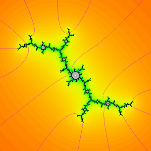
(a) Kokopelli

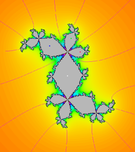
(b) (1/4)-rabbit

(c) worm

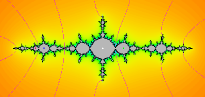
(d) double basilica

Figure 9: Four quadratic Julia sets with period $4$ critical orbit.

Lemma 5.16.

With $c_{j}$ and $\mathbb{E}$ as above, there are unique power series

$${\mathbf{u}}_{j}~{}=~{}-{\boldsymbol{\xi}}^{2}c_{j}\,+\,({\rm higher~{}order~{}terms})~{}\in~{}{\mathbb{E}}[[{\boldsymbol{\xi}}^{2}]]$$

which satisfy the required Equations $(\ref{e-u-condition})$. The corresponding escape regions are always ${\mathcal{I}}$-invariant.

Proof Outline. Suppose inductively that we can find series ${\mathbf{w}}_{1},\ldots{\mathbf{w}}_{p-1}$ satisfying $~{}E_{j}(\stackrel{{\scriptstyle\to}}{{{\mathbf{w}}}})\equiv 0~{}~{}({\rm mod}~{}{\boldsymbol{\xi}}^{2n})~{}$. To start the induction, for $n=3$ we can take $~{}{\mathbf{w}}_{j}=-{\boldsymbol{\xi}}^{2}c_{j}$.

Setting $~{}{\mathbf{w}}^{\prime}_{j}={\mathbf{w}}_{j}+{\boldsymbol{\xi}}^{2n-2}\delta_{j}~{}$, we find that

$$E_{j}(\stackrel{{\scriptstyle\to}}{{{\mathbf{w}}{}^{\prime}}})~{}\equiv~{}E_{j}(\stackrel{{\scriptstyle\to}}{{{\mathbf{w}}}})\,+\,{\boldsymbol{\xi}}^{2n}(\delta_{j+1}-\delta_{1}+2c_{j}\delta_{j})\quad({\rm mod}~{}{\boldsymbol{\xi}}^{2n+2})\,.$$

(Compare Lemma 5.4.) Now consider the linear map $~{}\stackrel{{\scriptstyle\to}}{{\delta}}\,\mapsto\,\stackrel{{\scriptstyle\to}}{{\delta{}^{\prime}}}~{}$ from ${\mathbb{E}}^{p-1}$ to itself, given by

$$\delta{}^{\prime}_{j}~{}=~{}\delta_{j+1}-\delta_{1}+2c_{j}\delta_{j}\,,$$ (28)

where $\delta_{p}=0$. If this transformation has non-zero determinant, then we can choose the $\delta_{j}$ so that $~{}E_{j}(\stackrel{{\scriptstyle\to}}{{{\mathbf{w}}{}^{\prime}}})~{}\equiv~{}0~{}~{}({\rm mod}~{}{\boldsymbol{\xi}}^{2n+2})$, thus completing the induction.

Now note that $c_{1}$ satisfies a monic polynomial equation with integer coefficients, and hence is an algebraic integer. Thus the ring ${\mathbb{Z}}[c_{1}]\subset{\mathbb{E}}$ is well behaved, with $~{}~{}1\not\equiv 0~{}~{}({\rm mod}~{}2\,{\mathbb{Z}}[c_{1}])$.  If we work modulo the ideal $2\,{\mathbb{Z}}[c_{1}]$, then the transformation of Equation (28) reduces to

$$\delta{}^{\prime}_{j}~{}\equiv~{}\delta_{j+1}-\delta_{1}\,,$$

which is easily seen to have determinant one. Thus Equation (28) also has non-zero determinant, which completes the proof.∎

Example 5.17 (Non-Primitive Regions).

More generally, consider any escape region ${\mathcal{E}}_{h}\subset{\mathcal{S}}_{p}$  such that the marked grid has period $n$ strictly less than the critical period $p$. Branner and Hubbard showed that every such region can be considered as a “satellite” of an escape region in $~{}{\mathcal{S}}_{n}$,  associated with some quadratic map of critical period $p/n$. (Compare Theorem 3.9.) Thus it is natural to start with a period $n$ solution $\stackrel{{\scriptstyle\to}}{{{\mathbf{w}}}}$ to the equations $~{}E_{j}(\stackrel{{\scriptstyle\to}}{{{\mathbf{w}}}})=0$,  and look for a period $~{}p~{}$ solution of the form $~{}\stackrel{{\scriptstyle\to}}{{{\mathbf{u}}}}\;=\;\stackrel{{\scriptstyle\to}}{{{\mathbf{w}}}}+\stackrel{{\scriptstyle\to}}{{{\boldsymbol{\delta}}}}$.

Theorem 5.18.

Suppose that $~{}\stackrel{{\scriptstyle\to}}{{{\mathbf{w}}}}~{}$ is a period $n$ solution to the equations$~{}E_{j}(\stackrel{{\scriptstyle\to}}{{{\mathbf{w}}}})=0$,  and that $~{}\stackrel{{\scriptstyle\to}}{{{\mathbf{u}}}}\,=\,\stackrel{{\scriptstyle\to}}{{{\mathbf{w}}}}+\stackrel{{\scriptstyle\to}}{{{\boldsymbol{\delta}}}}~{}$ is a period $~{}p~{}$ solution, with $~{}p\,>\,n$.Assume that $~{}{\boldsymbol{\delta}}_{j}=o({\mathbf{w}}_{j})$  for $~{}j\not\equiv 0~{}({\rm mod}~{}n)$,  and that $~{}{\mathbf{u}}_{j}={\boldsymbol{\delta}}_{j}=o(1)~{}$ for $~{}j\equiv 0~{}({\rm mod}~{}n)$.  Then for $~{}j\equiv 0~{}({\rm mod}~{}n)$, the leading monomial for $~{}{\mathbf{u}}_{j}={\boldsymbol{\delta}}_{j}~{}$ has the form

$${\mathbf{m}}_{n\,i}~{}=~{}c_{i}\,{\boldsymbol{\lambda}}\,,$$ (29)

where $~{}0~{}\mapsto~{}c_{1}~{}\mapsto~{}c_{2}~{}\mapsto~{}\cdots~{}\mapsto~{}c_{p/n-1}~{}\mapsto~{}0$  is the period $~{}p/n~{}$ critical orbit for an associated quadratic map,  and where $~{}{\boldsymbol{\lambda}}~{}$ is the fixed monomial

$${\boldsymbol{\lambda}}~{}=~{}-{\boldsymbol{\xi}}^{2n}/({\mathbf{m}}_{1}^{\textstyle\star}\,{\mathbf{m}}_{2}^{\textstyle\star}\,\cdots\,{\mathbf{m}}_{n-1}^{\textstyle\star})\,.$$ (30)

Here $~{}{\mathbf{m}}_{j}^{\textstyle\star}=(3\sigma_{j}-2){\mathbf{m}}_{j}~{}$ as in Equation (15). Thus, given the leading monomials for the ${\mathbf{w}}_{j}$, and given the complex constant $c_{1}$, we can compute the leading monomials for the $~{}{\mathbf{u}}_{j}$.  According to Theorem 5.1, the escape region $~{}{\mathcal{E}}_{h}~{}$ is then uniquely determined. Note that

$${\mathbf{m}}_{j}~{}=~{}{\mathbf{m}}_{n\,i+j}~{}\sim~{}{\mathbf{w}}_{n\,i+j}\qquad{\rm for}\qquad~{}0<j<n~{}\quad{\rm and}\quad 0<n\,i<p\,,$$ (31)

but that

$${\mathbf{m}}_{n\,i}~{}=~{}{\boldsymbol{\delta}}_{n\,i}\qquad{\rm with}\qquad{\mathbf{w}}_{n\,i}=0\,.$$ (32)

The following identity is an immediate consequence of Theorem 5.18, and will be useful in §6. Since $~{}{\mathbf{m}}_{n}^{\star}=-2{\mathbf{m}}_{n}$,  it follows that

$$\frac{{\mathbf{m}}_{1}^{\star}}{{\boldsymbol{\xi}}^{2}}\cdots\frac{{\mathbf{m}}_{n}^{\textstyle\star}}{{\boldsymbol{\xi}}^{2}}~{}=~{}2\,c_{1}\,.$$ (33)

The proof of Theorem 5.18 will depend on the following lemma.

Lemma 5.19.

For an escape region in ${\mathcal{S}}_{p}$ with grid period $~{}n$  and for$0<k<p$,  we have

$$~{}\sum_{j=1}^{k}\big{(}2-{\rm ord}({\mathbf{m}}_{j})\big{)}~{}\geq~{}0\,,$$

where this sum is is zero if and only if $~{}k~{}$ is congruent to zero modulo $~{}n\,$.It follows that the holomorphic function $~{}\prod_{j=1}^{k}(\xi^{2}/m_{j})$  of the local parameter $~{}\xi^{1/\mu}~{}$ tends to a well defined finite limit as the local parameter $~{}\xi^{1/\mu}~{}$ tends to zero,  and that this limit is non-zero if and only if $~{}k\equiv 0~{}({\rm mod}~{}n)$.

Proof. With notation as in Equation (20), let

$${\mathfrak{S}}_{j}~{}=~{}\sum_{\ell=0}^{\infty}\,{\rm MOD}\big{(}A_{\ell}(a_{j})\big{)}\,.$$

(Intuitively, the number $~{}{\mathfrak{S}}_{j}~{}$ is “large” if and only if the intersection of the puzzle pieces containing $~{}a_{j}~{}$ is “small”.) These numbers have two basic properties:

1. ${\mathfrak{S}}_{j+1}\,-\,{\mathfrak{S}}_{j}~{}=~{}{\rm ord}({\mathbf{m}}_{j})\;-\;2\,.$

2. If the period of the grid is $~{}n$,  then $~{}{\mathfrak{S}}_{1}~{}>~{}{\mathfrak{S}}_{j}~{}$ for $~{}1<j\leq n$.

To prove (a), note that $~{}{\rm MOD}\big{(}A_{\ell-1}(a_{j+1})\big{)}~{}$ is equal to either $~{}2\;{\rm MOD}\big{(}A_{\ell}(a_{j})\big{)}~{}$ or $~{}{\rm MOD}\big{(}A_{\ell}(a_{j})\big{)}$,  according as $~{}{\rm MOD}\big{(}A_{\ell}(a_{j})\big{)}~{}$ does or does not surround the critical point. Using Theorem 5.8, it follows that the difference $~{}{\mathfrak{S}}_{j+1}\,-\,{\mathfrak{S}}_{j}$  is equal to

$$\sum_{\ell=1}^{L_{0}(a_{j})}{\rm MOD}\big{(}A_{\ell}\big{)}~{}=~{}{\rm ord}({\mathbf{m}}_{j})\,,$$

minus the term $~{}{\rm MOD}\big{(}A_{0}(a_{j})\big{)}=2$.

To prove (b), note the formula

$${\rm MOD}\big{(}A_{\ell}(a_{j})\big{)}~{}=~{}2\;{\rm MOD}\big{(}A_{\ell+k}(a_{j-k})\big{)}\,,$$

where $~{}k\leq j~{}$ is the smallest positive integer such that $~{}A_{\ell+k}(a_{j-k})~{}$ surrounds the critical point. It follows that

$${\mathfrak{S}}_{1}~{}=~{}\sum_{\ell=1}^{\infty}\,2\;{\rm MOD}\big{(}A_{\ell}(a_{0})\big{)}\,,$$

while each $~{}{\mathfrak{S}}_{j}~{}$ with $~{}1<j<n~{}$ can be computed as a similar sum, but with some of the terms missing. The inequality (b) follows. Using both (a) and (b), we have the inequality

$$\sum_{j=1}^{k}\;\big{(}{\rm ord}({\mathbf{m}}_{j})-2\big{)}~{}=~{}{\mathfrak{S}}_{k+1}-{\mathfrak{S}}_{1}~{}<~{}0\qquad{\rm for}\qquad 1\leq k<n\,.$$

On the other hand, if $~{}n<p$,  then since $~{}{\mathfrak{S}}_{n+1}={\mathfrak{S}}_{1}$, the corresponding sum is zero. This proves Lemma 5.19 in the cases when $~{}k\leq n$.  The remaining cases follow immediately since $~{}{\mathfrak{S}}_{j+n}\,=\,{\mathfrak{S}}_{j}\,$. ∎

Remark 5.20.

One interesting consequence of this lemma, together with Theorem  5.8, is that multiplicity of an escape region depends only on its marked grid, and is independent of the period $p$. In particular, if a region in $~{}{\mathcal{S}}_{p}~{}$ is a “satellite” of a region in $~{}{\mathcal{S}}_{n}$  with $~{}n<p$,  then the two have the same multiplicity. (This statement would also follow easily from the Branner-Hubbard Theory.)

Proof of Theorem 5.18. Since $~{}E_{j}(\stackrel{{\scriptstyle\to}}{{{\mathbf{u}}}})=0~{}$ and $~{}E_{j}(\stackrel{{\scriptstyle\to}}{{{\mathbf{w}}}})=0$,  we have

$${\boldsymbol{\xi}}^{2}({\boldsymbol{\delta}}_{j+1}-{\boldsymbol{\delta}}_{1}) ~{}\sim~{} ~{}{\mathbf{m}}_{j}^{\textstyle\star}{\boldsymbol{\delta}}_{j}\qquad\quad{\rm if}\quad j\not\equiv 0~{}{\rm mod}~{}n\,,$$ (34)

$${\boldsymbol{\xi}}^{2}({\boldsymbol{\delta}}_{j+1}-{\boldsymbol{\delta}}_{1}) ~{}\sim~{} ~{}-{\boldsymbol{\delta}}_{j}^{\,2}~{}~{}\,\qquad\;{\rm if}\quad j=n\,i\,,$$ (35)

where the first equation follows from Lemma 5.4 and the second follows from Equation (14). We will prove by induction on $~{}j~{}$ that

$${\boldsymbol{\delta}}_{1}~{}\sim~{}\frac{{\boldsymbol{\xi}}^{2}}{{\mathbf{m}}_{1}^{\textstyle\star}}\cdots\frac{{\boldsymbol{\xi}}^{2}}{{\mathbf{m}}_{j-1}^{\textstyle\star}}\;{\boldsymbol{\delta}}_{j}$$ (36)

for $~{}1\leq j\leq n\,$. In fact, given this statement for some $~{}j<n$,  it follows from Lemma 5.19 that

$$\frac{{\boldsymbol{\xi}}^{2}}{{\mathbf{m}}_{j}^{\textstyle\star}}\;{\boldsymbol{\delta}}_{1}~{}=~{}o({\boldsymbol{\delta}}_{j})\,.$$

Equation (34) then implies that $~{}{\boldsymbol{\xi}}^{2}\,{\boldsymbol{\delta}}_{j+1}~{}\sim~{}{\mathbf{m}}_{j}^{\textstyle\star}\,{\boldsymbol{\delta}}_{j}$.  Substituting this equation into (36), the inductive statement that

$${\boldsymbol{\delta}}_{1}~{}\sim~{}\frac{{\boldsymbol{\xi}}^{2}}{{\mathbf{m}}_{1}^{\textstyle\star}}\cdots\frac{{\boldsymbol{\xi}}^{2}}{{\mathbf{m}}_{j}^{\textstyle\star}}\;{\boldsymbol{\delta}}_{j+1}$$

follows. This completes the proof of Equation (36).

It follows from this equation that

$${\rm ord}({\boldsymbol{\delta}}_{1})~{}=~{}2(n-1)\,+\,{\rm ord}({\boldsymbol{\delta}}_{n})\,-\,{\rm ord}({\mathbf{m}}_{1}\cdots{\mathbf{m}}_{n-1})\,.$$

On the other hand, it follows from Lemma 5.19 that

$${\rm ord}({\boldsymbol{\delta}}_{n})~{}=~{}{\rm ord}({\mathbf{m}}_{n})~{}=~{}2n\,-\,{\rm ord}({\mathbf{m}}_{1}\cdots{\mathbf{m}}_{n-1})\,.$$

Combining these two equations, it follows that

$${\rm ord}({\boldsymbol{\xi}}^{2}\,{\boldsymbol{\delta}}_{1})~{}=~{}{\rm ord}({\boldsymbol{\delta}}_{n}^{\,2}).$$

On the other hand, according to (35) we have

$${\boldsymbol{\xi}}^{2}({\boldsymbol{\delta}}_{n+1}-{\boldsymbol{\delta}}_{1})~{}\sim~{}-{\boldsymbol{\delta}}_{n}^{\,2}\,$$

Using the ultrametric inequality (13), this implies that $~{}\|{\boldsymbol{\delta}}_{n+1}\|\,\leq\,\|{\boldsymbol{\delta}}_{1}\|$,  or in other words $~{}{\rm ord}({\boldsymbol{\delta}}_{n+1})\,\geq\,{\rm ord}({\boldsymbol{\delta}}_{1})$.  The proof now divides into two cases.

Case 1.   If ${\rm ord}({\boldsymbol{\delta}}_{n+1})={\rm ord}({\boldsymbol{\delta}}_{1})$,  then arguing as above we see that

$${\boldsymbol{\delta}}_{n+1}~{}\sim~{}\frac{{\boldsymbol{\xi}}^{2}}{{\mathbf{m}}_{1}^{\textstyle\star}}\cdots\frac{{\boldsymbol{\xi}}^{2}}{{\mathbf{m}}_{n-1}^{\textstyle\star}}\;{\boldsymbol{\delta}}_{2n}\,.$$

again there is a dichotomy; but if $~{}{\rm ord}({\boldsymbol{\delta}}_{2n+1})={\rm ord}({\boldsymbol{\delta}}_{1})$,  then we can continue inductively. However, this cannot go on forever since $~{}{\boldsymbol{\delta}}_{p}=0$. Thus eventually we must reach:

Case 2.   For some $~{}i\geq 1$,  ${\rm ord}({\boldsymbol{\delta}}_{n\,i+1})\;>\;{\rm ord}({\boldsymbol{\delta}}_{1})$,  or in other words $~{}\|{\boldsymbol{\delta}}_{n\,i+1}\|~{}<\|{\boldsymbol{\delta}}_{1}\|$.  Then a straightforward induction, based on the statement that $~{}{\boldsymbol{\xi}}^{2}({\boldsymbol{\delta}}_{n\,i+j+1}-{\boldsymbol{\delta}}_{1})~{}\sim~{}{\mathbf{m}}_{j}^{\textstyle\star}{\boldsymbol{\delta}}_{n\,i+j}$,  shows that

$$\|{\boldsymbol{\delta}}_{n\,i+j}\|~{}<~{}\|{\boldsymbol{\delta}}_{j}\|~{}=~{}\left\|\frac{{\mathbf{m}}_{1}^{\textstyle\star}}{{\boldsymbol{\xi}}^{2}}\cdots\frac{{\mathbf{m}}_{j-1}^{\textstyle\star}}{{\boldsymbol{\xi}}^{2}}{\boldsymbol{\delta}}_{1}\right\|\,.$$

Taking $~{}j=n$,  since the $~{}\|{\boldsymbol{\delta}}_{n\,i}\|~{}$ with $~{}0<n\,i<p~{}$ all have the same norm by Theorem 5.8, it follows that $~{}n\,i+n=p$,  with $~{}{\boldsymbol{\delta}}_{p}=0$.

Now define the monomial $~{}{\boldsymbol{\lambda}}\in{\mathbb{C}}[{\boldsymbol{\xi}}^{1/\mu}]$  by Equation (30), and define $~{}c_{i}$  by Equation (29). Then it is not hard to check that the $c_{i}$ are complex numbers. Now note that

$${\boldsymbol{\xi}}^{2}\,{\boldsymbol{\delta}}_{n\,i+1}~{}\sim~{}{\boldsymbol{\xi}}^{2}\,\frac{{\boldsymbol{\xi}}^{2}}{{\mathbf{m}}_{1}^{\textstyle\star}}\cdots\frac{{\boldsymbol{\xi}}^{2}}{{\mathbf{m}}_{n-1}^{\textstyle\star}}\;{\boldsymbol{\delta}}_{n\,i+n}~{}\sim~{}{\boldsymbol{\lambda}}^{2}\,c_{i+1}\quad{\rm for}\quad n\,i<p-n\,,$$

while

$${\boldsymbol{\xi}}^{2}\,{\boldsymbol{\delta}}_{p-n+1}~{}=~{}o({\boldsymbol{\lambda}}^{\;2})\,.$$

Using the equation

$$~{}{\boldsymbol{\xi}}^{2}({\boldsymbol{\delta}}_{n\,i+1}-{\boldsymbol{\delta}}_{1})~{}\sim~{}-{\boldsymbol{\delta}}_{n\,i}^{\;2}~{}\sim~{}-{\boldsymbol{\lambda}}^{2}\,c_{i}^{\,2}\,,$$

it follows that

$$c_{i+1}~{}=~{}c_{i}^{\;2}\,+\,c_{1}\,,$$

with $~{}c_{p/n}\,=\,0\,$. This completes the proof of Theorem 5.18.∎

Remark 5.21 (An Empirical Algorithm).

How can we locate examples of maps $~{}F_{a,\,v}$  belonging to some unknown escape region? Choosing an arbitrary value of $~{}a~{}$ (with $~{}|a|~{}$ not too small), given the kneading sequence, and given a rough approximation $~{}v^{\prime}\,\approx\,~{}v$,  the following algorithm is supposed to converge to the precise value of $~{}v$.  It seems quite useful in practice. (In fact, it often eventually converges, starting with a completely random $~{}v^{\prime}$.)  However, we have no proof of convergence, even if the initial $~{}v^{\prime}~{}$ is very close to the correct value. Furthermore, there are examples (near the boundary of an escape region) where the algorithm converges to a map with the wrong kneading sequence.

Given the required kneading sequence $~{}\stackrel{{\scriptstyle\to}}{{\sigma}}$,  consider the generically defined holomorphic maps $~{}\Psi_{j}\,:\,{\mathbb{C}}^{3}~{}\to~{}{\mathbb{C}}~{}$ defined by

$$\Psi_{j}(w_{1},\,w_{j},\,w_{j+1})~{}=~{}\begin{cases}w_{j}\sqrt{\frac{\xi^{2}(w_{j+1}-w_{1})}{w_{j}^{\;2}(w_{j}-1)}}&{\rm if}\quad\sigma_{j}=0\,,\\ \\ 1\;+\;\frac{\xi^{2}(w_{j+1}-w_{1})}{w_{j}^{\,2}}&{\rm if}\quad\sigma_{j}=1\,,\end{cases}$$

taking that branch of the square root function which is defined on the right half-plane. Then it is easy to check that

$$w_{j}~{}=~{}\Psi_{j}(w_{1},\,w_{j},\,w_{j+1})\qquad{\rm if~{}and~{}only~{}if}\qquad E_{j}(\stackrel{{\scriptstyle\to}}{{w}})=0\,.$$

Choosing some $~{}\xi=1/(3a)$,  and given some approximate solution to the equations $~{}E_{j}(\stackrel{{\scriptstyle\to}}{{w}})=0$,  proceed as follows. Replace $~{}w_{j}~{}$ by $~{}\Psi_{j}(w_{1},\,w_{j},\,w_{j+1})$, starting with $~{}j=p-1$,  then with $~{}j=p-2$,  and so on until $~{}j=1$. Then repeat this cycle until the sequence has converged to machine accuracy, or until you lose patience. If the sequence does converge, then the limit will certainly describe some map in $~{}{\mathcal{S}}_{p}$,  and it is easy to check whether or not it has the required kneading sequence.

If we start only with a pair $~{}(a,\,v)$  and a kneading sequence, we can first compute the partial orbit

$$a~{}=~{}a_{0}~{}\mapsto~{}a_{1}~{}\mapsto~{}\cdots~{}\mapsto a_{p-1}\,,$$

then set $~{}w_{j}=(a-a_{j})/(3a),$  and proceed as above.

6 Canonical Parameters and Escape Regions.

Recall from §2 that the canonical coordinate $~{}t=t(a,v)~{}$ on $~{}{\mathcal{S}}_{p}~{}$ is defined locally, up to an additive constant, by the formula

$$dt~{}=~{}\frac{da}{\partial\Phi_{p}/\partial v}\qquad{\rm where}\qquad\Phi_{p}(a,v)~{}=~{}F_{a,v}^{\circ p}(a)-a\,.$$ (37)

In particular, the differential $~{}dt~{}$ is uniquely defined, holomorphic, and non-zero everywhere on the curve ${\mathcal{S}}_{p}$. We will prove that the residue

$$\frac{1}{2\pi i}\oint dt$$ (38)

at the ideal point is zero, so that the indefinite integral $~{}t\;=\;\int dt~{}$ is well defined, up to an additive constant, throughout the escape region. (However, as noted in Remark 2.1, it usually cannot be defined as a global function on $~{}{\mathcal{S}}_{p}$.)

Furthermore, whenever the kneading sequence is non-trivial, we will show that the function $~{}t~{}$ has a removable singularity, and hence extends to a smooth holomorphic function which is defined and finite also at the ideal point. On the other hand, in the case of a trivial kneading sequence $~{}000\cdots 0$,  the function $~{}t~{}$ has a pole at the ideal point, and in fact is asymptotic to some constant multiple of $a$. We will first need the following.

Definition 6.1.

For each $~{}j\geq 0$,  consider the polynomial expression

$$\psi_{j+1}(X_{1},\,\ldots,\,X_{j})~{}=~{}\hskip 227.62204pt$$

$$X_{1}X_{2}X_{3}X_{4}\cdots X_{j}~{}+~{}X_{2}X_{3}X_{4}\cdots X_{j}~{}+~{}X_{3}X_{4}\cdots X_{j}~{}+~{}\ldots~{}+X_{j}~{}+~{}1$$

in $j$ variables. These can be defined inductively by the formula

$$~{}~{}\psi_{j+1}(X_{1},\,\ldots,\,X_{j})~{}=~{}\psi_{j}(X_{1},\,\ldots,\,X_{j-1})\,X_{j}\,+\,1\,,$$

starting with $~{}\psi_{1}(~{})~{}=~{}1$.

We will prove the following statement. It will be convenient to make use of both of the variables $~{}a~{}$ and $~{}\xi=1/(3a)$. As in Remark 4.1, a choice of anchoring for $~{}{\mathcal{E}}_{h}~{}$ determines a choice of local parameter $~{}\xi^{1/\mu}\,=\,1/(3a)^{1/\mu}~{}$ near the ideal point.

Theorem 6.2.

Let $~{}n\leq p$  be the grid period for the escape region$~{}{\mathcal{E}}_{h}\subset{\mathcal{S}}_{p}\,$,  and let   $0\mapsto c_{1}\mapsto c_{2}\mapsto\cdots\mapsto c_{r-1}\mapsto 0$   be the critical orbit for the associated quadratic map, where $~{}r=p/n\geq 1$.  Then the derivative $~{}da/dt~{}$ is given by the asymptotic formula

$$da/dt~{}\sim~{}\psi_{r}(2c_{1},\ldots,2c_{r-1})\,\prod_{j=1}^{n-1}\,\frac{m_{j}^{\textstyle\star}}{\xi^{2}}\qquad{\rm as}\qquad\xi\to 0\quad({\rm or~{}as}\quad|a|\to\infty)\,,$$

where $~{}m_{j}^{\textstyle\star}=(3\sigma_{j}-2)m_{j}$  as in Equation $(\ref{e-m*})$, and where $~{}\psi_{r}(2c_{1},\cdots,2c_{r-1})$ is a non-zero complex number.

Note that

$$d\xi/dt~{}=~{}(d\xi/da)(da/dt)~{}=~{}-3\xi^{2}\,da/dt\,.$$

Thus it follows from Theorem 6.2 that $~{}t~{}$ can be expressed as an indefinite integral

$$t~{}=~{}\int dt \sim \int\frac{da}{\psi_{r}(2c_{1},\ldots,2c_{r-1})}\prod_{j=1}^{n-1}\frac{\xi^{2}}{m_{j}^{\textstyle\star}}~{}~{}x$$ (39)

$$~{}~{}=~{} \int\frac{-d\xi~{}}{~{}3\,\xi^{2}\,\psi_{r}(2c_{1},\ldots,2c_{r-1})}\prod_{j=1}^{n-1}\frac{\xi^{2}}{m_{j}^{\textstyle\star}}\;.$$

If the kneading sequence is non-trivial, or in other words if $~{}n>1$,  then Lemma 5.19 implies that the product $~{}\prod(\xi^{2}/m^{\textstyle\star}_{j})~{}$ is a bounded holomorphic function of the local parameter $~{}\xi^{1/\mu}$  in a neighborhood of the ideal point, and hence that $~{}t~{}$ can be defined as a bounded holomorphic function of $\xi^{1/\mu}$.  On the other hand, if the kneading sequence is trivial so that $~{}n=1$,  then this integral has a pole at the ideal point, and in fact it follows easily that

$$t~{}~{}\sim~{}~{}\frac{a}{\psi_{p}(2c_{1},\ldots,2c_{p-1})}~{}.$$ (40)

If we choose the constant of integration in the indefinite integral of Equation (39) appropriately, then we can express $t$ as a holomorphic function of the form

$$t(\xi^{1/\mu})~{}=~{}\beta\,\xi^{\nu/\mu}\;+\;\rm{(higher~{}order~{}terms)}\;,$$ (41)

where $~{}\beta~{}$ is a non-zero complex coefficient and $~{}\nu~{}$ is a non-zero integer.

Definition 6.3.

This integer $~{}\nu\neq 0~{}$ will be called the winding number(or the  ramification index)  of the escape region over the $~{}t$-plane. In fact,as we make a simple loop in the positive direction in the $\xi^{1/\mu}$-parameter plane, the corresponding point in the $~{}t$-plane will wind $~{}\nu~{}$ times around the origin. Thus $~{}\nu>0~{}$ when the kneading sequence $~{}\stackrel{{\scriptstyle\to}}{{\sigma}}~{}$ is non-trivial;  but $~{}\nu=-1$  when $~{}\stackrel{{\scriptstyle\to}}{{\sigma}}\;=\;(0,\ldots,0)$.  In either case, it follows that any choice of $~{}t^{1/\nu}~{}$ can be used as a local uniformizing parameter near the ideal point. It follows easily from Equation (39) that this winding number is given by the formula

$$\nu~{}=~{}\big{(}2n\,-\,3\,-\,{\rm ord}(m_{1}\cdots m_{n-1})\big{)}\,\mu\,.$$ (42)

Using Theorem 5.8, it follows that $~{}\nu~{}$ depends only on the marked grid.

Proof of Theorem 6.2. The argument will be based on the following computations. Start with the periodic orbit   $a=a_{0}\mapsto a_{1}\mapsto\cdots$,  where

$$a_{j+1}=F_{a,v}(a_{j})~{}=~{}a_{j}^{3}-3a^{2}a_{j}+2a^{3}+v\,.$$

It will be convenient to set

$$X_{j} ~{}=~{} \frac{\partial a_{j+1}}{\partial a_{j}}~{}=~{}3(a_{j}^{2}-a^{2})\,,$$ (43)

$$Y_{j+1} ~{}=~{} \frac{\partial a_{j+1}}{\partial v}~{}=~{}\frac{\partial a_{j+1}}{\partial a_{j}}\,\frac{\partial a_{j}}{\partial v}\,+\,1\,.$$ (44)

In other words

$$Y_{j+1}~{}=~{}Y_{j}X_{j}\,+\,1\qquad{\rm with}\qquad Y_{1}~{}=~{}\frac{\partial a_{1}}{\partial v}~{}=~{}1\,,$$ (45)

or briefly

$$Y_{j+1}~{}=~{}\psi_{j+1}(X_{1},\,\ldots,\,X_{j})\,,$$ (46)

using Definition 6.1.

Denoting $~{}~{}\Phi_{p}(a,v)\;=\;F_{a,v}^{\circ p}-a~{}~{}$ briefly by $~{}a_{p}-a$,  and noting that$~{}\partial a/\partial v=0$,  we see from Equation (37) that

$$\frac{\partial\Phi_{p}(a,v)}{\partial v}~{}=~{}\frac{\partial a_{p}}{\partial v}~{}=~{}Y_{p}~{}=~{}\psi_{p}(X_{1},\,\ldots,\,X_{p-1})\,,$$

and hence that

$$dt~{}=~{}\frac{da}{\partial\Phi_{p}/\partial v}~{}=~{}\frac{da}{Y_{p}}\qquad{\rm or}\qquad da/dt~{}=~{}Y_{p}\,.$$

Thus, in order to prove Theorem 6.2, we must find an asymptotic expression for $~{}Y_{p}$.

Substituting $~{}a=1/3\,\xi~{}$ and $~{}a_{j}=(1-3u_{j})a$  in Equation (43),  we easily obtain

$$X_{j}~{}=~{}\frac{3u_{j}^{\,2}-2u_{j}}{\xi^{2}}~{}\sim~{}\frac{m_{j}^{\textstyle\star}}{\xi^{2}}~{},$$ (47)

where $~{}m_{j}^{\textstyle\star}=(3\sigma_{j}-2)m_{j}~{}$ is the leading term in the series expansion for $~{}3u_{j}^{\,2}-2u_{j}~{}$ as described in Equation (15),  so that $~{}m_{j}^{\textstyle\star}\sim 3u_{j}^{\,2}-2u_{j}$. We next show by induction on $~{}j~{}$ that

$$Y_{j}~{}\sim~{}X_{1}\cdots X_{j-1}~{}\sim~{}\frac{m_{1}^{\textstyle\star}}{\xi^{2}}\cdots\frac{m_{j-1}^{\textstyle\star}}{\xi^{2}}\qquad{\rm for}\qquad j\leq n\;.$$

In fact this expression for a given value of $~{}j~{}$ implies that

$$X_{j}Y_{j}~{}\sim~{}X_{1}X_{2}\cdots X_{j}\,,$$

where this expression has a pole at the origin by Lemma 5.19. Hence it is asymptotic to $~{}X_{j}Y_{j}+1=Y_{j+1}$,  which completes the induction. In particular, it follows that $~{}Y_{n}\;\sim\;\prod\limits_{j=1}^{n-1}\displaystyle{\big{(}\frac{m_{j}^{\textstyle\star}}{\xi^{2}}\big{)}}$.  In the primitive case $~{}p=n$,  this completes the proof of Theorem 6.2.

Suppose then that $~{}p>n$.  By Equations (29) and (30) of Theorem 5.18, we have $~{}m_{n}^{\textstyle\star}\;=\;-2\,c_{1}$,  and hence

$$X_{n}Y_{n}~{}\sim~{}(m_{1}^{\textstyle\star}/\xi^{2})\cdots(m_{n}^{\textstyle\star}/\xi^{2})~{}=~{}2c_{1}\,,$$

and therefore $~{}Y_{n+1}~{}\sim~{}2\,c_{1}+1~{}=~{}\psi_{2}(2\,c_{1})\,.$ Suppose inductively that

$$Y_{n\,i+1}~{}\sim~{}\psi_{i+1}(2\,c_{1},\ldots,2\,c_{i})\,.$$

Then by induction on $~{}j~{}$ we see that

$$Y_{n\,i+j}~{}\sim~{}\psi_{i+1}(2\,c_{1},\cdots,2\,c_{i})\,X_{1}\cdots X_{j-1}~{}\sim~{}\psi_{i+1}(2\,c_{1},\cdots,2\,c_{i})\,\frac{m_{1}^{\textstyle\star}}{\xi^{2}}\cdots\frac{m_{j-1}^{\textstyle\star}}{\xi^{2}}$$

for $~{}j\leq n\;.~{}$ Taking $~{}j=n~{}$ and $~{}i=r-1$  so that $~{}ni+j=p$,  this completes the proof.∎

$p$	$r$	$\stackrel{{\scriptstyle\to}}{{\sigma}}$	$m_{1}$	$m_{2}$	$m_{3}$	$t\sim$	$\nu$	$\mu$	$\#$	sym
2	1	$\overline{10}$	1			$-\xi/3$	1	1	1	$\pm$
3	1	$\overline{110}$	1	1		$-\xi^{3}/9$	3	1	1	$\pm$
3	1	$\overline{100}$	1	$\pm\xi$		$\pm\xi^{2}/12$	2	1	2	$+$
3	1	$\overline{010}$	$\pm i\xi$	1		$\mp i\xi^{2}/12$	2	1	2	$-$
4	2	$\overline{1010}$	1	$\xi^{4}$	1	$\xi/3$	1	1	1	$\pm$
4	1	$\overline{1110}$	1	1	1	$-\xi^{5}/15$	5	1	1	$\pm$
4	1	$\overline{1100}$	1	1	$\pm\xi$	$\pm\xi^{4}/24$	4	1	2	$+$
4	1	$\overline{0110}$	$\pm i\xi$	1	1	$\mp i\xi^{4}/24$	4	1	2	$-$
4	1	$\overline{1000}\,{\rm s}$	1	$\pm\xi$	$\mp\xi$	$\;\;\xi^{3}/36$	3	1	2	$+$
4	1	$\overline{1000}\,{\rm t}$	1	$\pm\xi$	$\pm\xi$	$-\xi^{3}/36$	3	1	2	$+$
4	1	$\overline{0100}$	$\omega^{2}\xi$	1	$-\omega\xi^{3/2}$	$-\omega\xi^{5/2}/30$	5	2	2	$-$
4	1	$\overline{0010}$	$\omega\xi^{3/2}$	$-\omega^{2}\xi$	1	$-\omega\xi^{5/2}/30$	5	2	2	$-$

Table 6.4: Escape regions in $~{}{\mathcal{S}}_{p}~{}$ with nontrivial kneading sequence for $p\leq 4$. Here $~{}r=p/n~{}$ is the critical period for the associated quadratic map, and $\#$ is the number of such regions. In the last column, $+$ stands for symmetry under complex conjugation so that $~{}{\mathcal{E}}_{h}=\overline{\mathcal{E}}_{h}$, and $-$ stands for symmetry under ${\mathcal{I}}$ composed with complex conjugation. $($Compare §$\ref{s-real}.)$ The symbol $~{}\omega~{}$ stands for any $4$-th root of $-1$. Note that the exponent of $~{}\xi~{}$ in the $~{}t\!\sim~{}$ column, is equal to $\nu/\mu$. In all of these cases, $\nu$ and $\mu$ are relatively prime.

7 The Euler Characteristic

Using the meromorphic 2-form $~{}dt$,  it is not difficult to calculate the Euler characteristic of $~{}{\mathcal{S}}_{p}~{}$ or of $~{}\overline{\mathcal{S}}_{p}$. Here is a preliminary result.

Lemma 7.1.

The Euler characteristic of the compact curve $~{}\overline{\mathcal{S}}_{p}~{}$ can be expressed as

$$\chi(\overline{\mathcal{S}}_{p})~{}=\sum_{\rm escape~{}regions}(1-\nu)\,,$$

to be summed over all escape regions in $~{}{\mathcal{S}}_{p}$.  Here $~{}\nu$  is the winding number of Definition 6.3,  as computed in Equation $(\ref{e-nu=})$. It follows that the Euler characteristic of the affine curve $~{}{\mathcal{S}}_{p}~{}$ is given by

$$\chi({\mathcal{S}}_{p})~{}=~{}-\sum\nu\,.$$

Note: By definition, the Euler characteristic $~{}\chi({\mathcal{S}}_{p})~{}$ is equal to the difference of Betti numbers, $~{}{\rm rank}\big{(}H^{0}({\mathcal{S}}_{p})\big{)}\,-\,{\rm rank}\big{(}H^{1}({\mathcal{S}}_{p})\big{)}$.  If we use Čech cohomology, then the Betti numbers of $~{}{\mathcal{S}}_{p}~{}$ can be identified with the Betti numbers of the connectedness locus $~{}{\mathcal{C}}({\mathcal{S}}_{p})$.

Proof of Lemma 7.1. Given any meromorphic 1-form on a compact (not necessarily connected) Riemann surface $~{}{\mathcal{S}}$,  we can compute the Euler characteristic of $~{}{\mathcal{S}}$  in terms of the zeros and poles of the 1-form counted with multiplicity, by the formula

$$\chi({\mathcal{S}})~{}~{}=~{}~{}\#({\rm poles})\,-\,\#({\rm zeros})\,.$$

We can apply this formula to the meromorphic 1-form $~{}dt~{}$ on the compact curve $\overline{\mathcal{S}}_{p}$.  Since the only zeros and poles of $~{}dt~{}$ are at the ideal points, we need only compute the order of the zero or pole at each ideal point, using $~{}\xi^{1/\mu}$  as local uniformizing parameter. In fact, using Theorem 6.2, we see easily that $~{}dt~{}$ has a zero of order $\nu-1\geq 0$ whenever the kneading sequence is non-trivial, and a pole of order $~{}1-\nu=2~{}$ when the kneading sequence is trivial. This completes the proof for $~{}\overline{\mathcal{S}}_{p}$. The corresponding formula for $~{}{\mathcal{S}}_{p}$  follows, since each point which is removed decreases $~{}\chi~{}$ by one.∎

Note: Based on this result, combined with a combinatorial method to compute the number of escape regions associated with each marked grid, Aaron Schiff at the University of Illinois Chicago, under the supervision of Laura DeMarco, has written a program to compute the Euler characteristic of $\overline{\mathcal{S}}_{p}$ for many values of $~{}p$.

The formula for $~{}\chi~{}$ can be simplified as follows. Let $~{}d_{p}~{}$ be the degree of the affine curve ${\mathcal{S}}_{p}$, defined inductively by the formula

$$\sum_{n|p}d_{n}~{}=~{}3^{p-1}\,.$$

Theorem 7.2.

The Euler characteristic of the affine curve $~{}{\mathcal{S}}_{p}$ is given by

$$\chi({\mathcal{S}}_{p})~{}=~{}(2-p)\,d_{p}\,.$$

Hence the Euler characteristic of $~{}\overline{{\mathcal{S}}_{p}}$  is

$$\chi({\mathcal{S}}_{p})~{}=~{}N_{p}\,+\,(2-p)\,d_{p}\,,$$

where $N_{p}$ is the number of escape regions $($ = number of puncture points$)$.

As examples, for $~{}p\leq 4$  we have the following table.

$p$	$d_{p}$	$(2-p)\times d_{p}$	$~{}~{}N_{p}$	$\chi(\overline{\mathcal{S}}_{p})$
1	1	$1\times 1$	1	2
2	2	$0\times 2$	2	2
3	8	$-1\times 8$	8	0
4	24	$-2\times 24$	20	-28

Table 7.3:

The proof will depend on the following. Let $~{}\widehat{a}\in{\mathbb{C}}~{}$ be an arbitrary constant. Then the line $~{}\{(a,v)~{};~{}a=\widehat{a}\}~{}$ intersects $~{}{\mathcal{S}}_{p}~{}$ in  $~{}d_{p}~{}$ points, counted with multiplicity. The corresponding values of $~{}v~{}$ will be denoted by $~{}v_{1},\,\ldots,\,v_{d_{p}}$.

Lemma 7.4.

For each $~{}0<j<p$,  the product

$$\prod_{k=1}^{d_{p}}~{}\Big{(}\widehat{a}-F_{\widehat{a},v_{k}}^{\circ j}(\widehat{a})\Big{)}$$ (48)

is a non-zero complex constant $($conjecturally equal to $+1\,)$.

Proof. The numbers $~{}v_{k}$  are the roots of a polynomial equation with coefficients in $~{}{\mathbb{C}}[\widehat{a}]$.  Since Equation (48) is a symmetric polynomial function of the $~{}v_{k}\,$,  it can be expressed as a polynomial in the elementary symmetric functions, and hence can be expressed as a polynomial function of $~{}\widehat{a}$.  Since this function has no zeros, it is a non-zero constant.∎

Proof of Theorem 7.2. Using Lemma 7.1, it suffices to prove the identity

$$\sum_{h=1}^{N_{p}}\nu({\mathcal{E}}_{h})~{}=~{}(p-2)\,d_{p}\,.$$

By Equation (42) together with Lemma 5.19, we have

$$\nu/\mu~{}=~{}-1+\sum_{1}^{n-1}\Big{(}2-{\rm ord}({\mathbf{m}}_{j})\Big{)}~{}=~{}-1+\sum_{1}^{p-1}\Big{(}2-{\rm ord}({\mathbf{m}}_{j})\Big{)}\,.$$

Since $~{}~{}2-{\rm ord}({\mathbf{m}}_{j})\,=\,1-{\rm ord}({\mathbf{a}}-{\mathbf{a}}_{j})$,  it follows that

$$\nu/\mu~{}=~{}p-2\,-\,{\rm ord}\Big{(}({\mathbf{a}}-{\mathbf{a}}_{1})({\mathbf{a}}-{\mathbf{a}}_{2})\cdots({\mathbf{a}}-{\mathbf{a}}_{p-1})\Big{)}\,.$$ (49)

Choosing some large $\widehat{a}$ and summing over the $d$ intersection points, each escape region contributes $\mu$ copies of Equation $(\ref{e-numu})$. Therefore the left side of the equation adds up to $\sum_{1}^{N_{p}}\nu$. The first term on the right side adds up to$(p-2)d_{p}$.  Since it follows from Lemma 7.4 that the second term on the right adds up to zero, this proves Theorem 7.2.∎

8 Topology of ${\mathcal{S}}_{p}$

Conjecturally the curve ${\mathcal{S}}_{p}$ is irreducible (= connected) for all periods $~{}p$. Whenever this curve is connected, we can use the results of §7 to compute the genus of the closed Riemann surface $~{}\overline{\mathcal{S}}_{p}$,  and the first Betti number of the open surface $~{}{\mathcal{S}}_{p}$  or of its connectedness locus. However, unfortunately we do not have a proof of connectivity for any period $~{}p>4$. (In this connection, it is interesting to note that any connected component of ${\mathcal{S}}_{p}$ for $p>1$ must contain hyperbolic components of Types A, B, C and D, as well as escape components. In fact the zeros and poles of the meromorphic function $~{}(a,v)\mapsto a\in{\mathbb{C}}~{}$ yield centers of Type A and ideal points, while the zeros of the functions $~{}v+a~{}$ and $~{}F(-a)+a~{}$ yield centers of Type B and D. With a little more work, one can find centers of Type C as well.)

For $p\leq 4$, we are able to prove connectivity, and to provide a more direct computation of the genus, by constructing an explicit cell subdivision of $\overline{\mathcal{S}}_{p}$ with the ideal points as vertices. As an example, Figure 9 shows part of the universal covering space of the torus $~{}\overline{\mathcal{S}}_{3}$.  The ideal point in each escape region has been marked with a black dot. Joining neighboring ideal points by more or less straight lines, we can easily cut the entire plane up into triangular 2-cells. The corresponding triangulation of $~{}\overline{\mathcal{S}}_{3}~{}$ itself has 16 triangles, 24 edges, and 8 vertices.

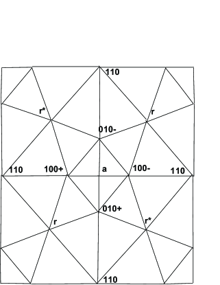
Figure 10: Universal covering space of $\overline{\mathcal{S}}_{3}$. Here $\bf r$ stands for the ideal point in the $(1/3)$-rabbit region, $\bf r^{*}$ for its complex conjugate, and $\bf a$ for the ideal point in the airplane region. Note that the $180^{\circ}$ rotation ${\mathcal{I}}$ interchanges $\overline{100}+$ and $\overline{100}-$, and also interchanges $\overline{010}+$ and $\overline{010}-$, but fixes the remaining four ideal points.

This cell structure can be described as follows. Let $~{}{\mathcal{S}}~{}$ stand either for the curve $~{}\overline{\mathcal{S}}_{p}~{}$ or for the quotient curve $~{}\overline{\mathcal{S}}_{p}/{\mathcal{I}}$,  where $~{}{\mathcal{I}}:F_{a,v}\mapsto F_{-a,-v}~{}$ is the canonical involution. Let $~{}V~{}$ be the finite set consisting of all ideal points in $~{}{\mathcal{S}}$, and for each $~{}{\mathbf{v}}\in V~{}$ let $~{}{\mathcal{E}}_{\mathbf{v}}\subset{\mathcal{S}}$  be the associated escape region. Given two points $~{}{\mathbf{v}},\,{\mathbf{v}}^{\prime}\in V$,  consider all paths $P\subset{\mathcal{S}}$ from ${\mathbf{v}}$ to ${\mathbf{v}}^{\prime}$ which satisfy the following two conditions:

• $~{}P~{}$ is disjoint from the closure $\overline{\mathcal{E}}_{\mathbf{w}}$ for all ${\mathbf{w}}$ other than ${\mathbf{v}}$ and ${\mathbf{v}}^{\prime}$.

• The intersections $P\cap{\mathcal{E}}_{\mathbf{v}}$ and $P\cap{\mathcal{E}}_{{\mathbf{v}}^{\prime}}$ are both connected.

Choose one representative from each homotopy class of such paths $P$ as an edge from ${\mathbf{v}}$ to ${\mathbf{v}}^{\prime}$. Conjecturally, these vertices and edges form the 1-skeleton of the required cell subdivision. In any case, this certainly works for periods $p\leq 4$.

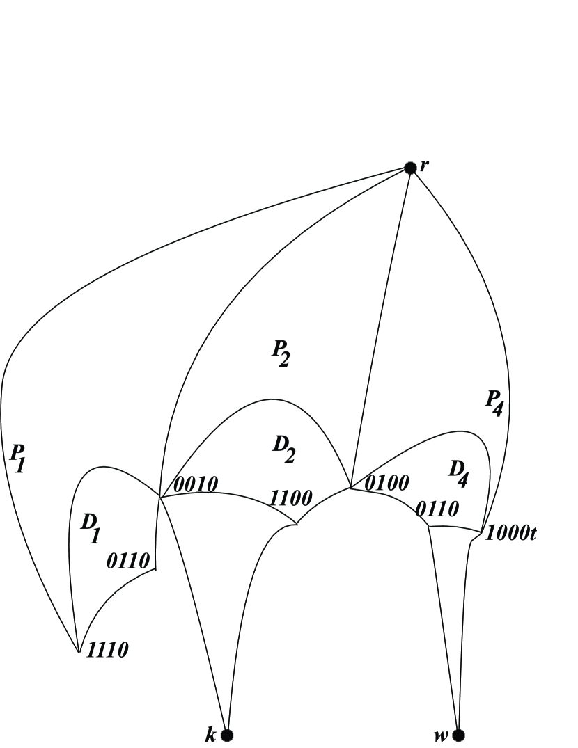
Figure 11: Part of $\overline{\mathcal{S}}_{4}$, illustrating the cell structure. Here $k,\,r,\,w$ stand for the kokopelli, $(1/4)$-rabbit, and worm centers. The three top triangles are centered at parabolic points $P_{i}$, the next three at Type D centers $D_{i}$, and the bottom two at Type A centers.

As an example, the cell structure for the curve $~{}\overline{\mathcal{S}}_{4}/{\mathcal{I}}~{}$ has:

14 vertices (= ideal points), 68 edges, and  44 faces.

See Figure 12 for a diagram illustrating part of this cell complex, including 22 of the 44 faces and 12 of the 14 vertices. (Most of these vertices are shown in multiple copies.) The only vertices which are not included are the complex conjugates of $~{}r~{}$ and $~{}k$, which will be denoted by $~{}r^{*}~{}$ and $~{}k^{*}$.  (All of the other vertices are self-conjugate.) One can obtain the full cell complex from this partial diagram in three steps as follows:

Figure 12: Schematic picture of the cell structure for half of $~{}\overline{\mathcal{S}}_{4}/{\mathcal{I}}$.  Here each vertex is represented by a circle containing a brief label for the corresponding escape region. In particular, the kneading sequences $~{}\overline{0010}\,,~{}\overline{0100}\,,~{}\ldots\,,~{}\overline{1110}~{}$ in lexicographical order are labeled simply by the integers $1,\,2\,,\ldots,\,7$.

• Take a second “complex conjugate” copy of this diagram, with the two interior vertices of the complex conjugate diagram labeled as $~{}r^{*}$  and $~{}k^{*}$  respectively.

• Glue these two diagrams together along the ten emphasized edges. (Each emphasized edge represents a one real parameter family of mappings $~{}F_{a,v}~{}$, where $~{}a~{}$ and $~{}v~{}$ are either both real or both pure imaginary. Compare §9.) The resulting surface will have twelve temporary boundary circles, labeled in pairs by Greek letters.

• Now glue each of these boundary circles onto the other boundary circle which has the same label, matching the two so that the result will be an oriented surface. (In most cases, this means gluing an edge from the original diagram onto an edge from the complex conjugate diagram. However, there is one exception: Each edge with label $\beta$ must be glued to the other $\beta$ edge from the same diagram.)

The result of this construction will be a closed oriented surface. In particular, the given edge identifications will force the required vertex identifications.

Evidently complex conjugation operates as an orientation reversing involution of this surface. The fixed points of this involution (made up out of the ten emphasized edges in Figure 12) consist of two circles, which represent all possible “real” cubic maps in $~{}{\mathcal{S}}_{4}/{\mathcal{I}}$. (Compare §9.) One of these circles has just two vertices $\,1\,$ and $\,3\,$,  while the other has eight vertices, listed in cyclic order as $~{}~{}2\,,~{}{\rm w}\,,~{}4_{\rm t}\,,~{}5\,,~{}7\,,~{}6\,,~{}4_{\rm s}\,,~{}{\rm d}\,$.

Note that this combinatorial structure is closely related to the dynamics:At the center of each triangular face, three escape regions come together, either at a parabolic point or around a hyperbolic component of Type A or D. Similarly, at the center of each quadrilateral face, four escape regions come together around a hyperbolic component of Type B.

Given this cell structure, we can easily compute the Euler characteristic

$$\chi(\overline{\mathcal{S}}_{4}/{\mathcal{I}})~{}=~{}14-68+44~{}=~{}-10\,.$$

Setting $~{}\chi=2-2g$,  this corresponds to a genus of $~{}g(\overline{\mathcal{S}}_{4}/{\mathcal{I}})\,=\,6$. The curve $~{}\overline{\mathcal{S}}_{4}~{}$ itself is a two-fold branched covering of $~{}\overline{\mathcal{S}}_{4}/{\mathcal{I}}$,   ramified over the eight of the vertices (namely, those labeled  d, k, r, w, 5, and 7 in Figure 12, as well as the conjugate vertices $k^{*}$ and $r^{*}$). Thus the induced cell subdivision has Euler characteristic

$$\chi\big{(}\,\overline{\mathcal{S}}_{4}\big{)}~{}=~{}2-2g(\overline{\mathcal{S}}_{4})~{}=~{}(2\cdot 14-8)-2\cdot 68+2\cdot 44~{}=~{}-28\,,$$

corresponding to genus 15. (Compare Table 7.3.)

9 Real Cubic Maps

It will be convenient to say that the cubic map $F_{a,\,v}$ is  real  if $a$ and $v$ are real, so that $~{}F_{a,v}({\mathbb{R}})={\mathbb{R}}$,  and  pure imaginary  if $~{}a~{}$ and $~{}v~{}$ are pure imaginary,  so that $F_{a,v}(i{\mathbb{R}})=i{\mathbb{R}}$.

(In fact, every “pure imaginary” map $F_{ia,\,iv}$ is conjugate to a map

$$x~{}\mapsto~{}F_{ia,\,iv}(ix)/i~{}=~{}-x^{3}\;+\;3a^{2}\,x\;+\;(-2a^{3}+v)$$

with real coefficients. However, the coefficient of the cubic term in this conjugate map is $-1$ rather than $+1$. This leads to a drastic difference in real dynamical behavior.)

Note that the space of monic centered complex cubic polynomials has two commuting anti-holomorphic involutions: namely complex conjugation, which will be denoted by

$${\mathfrak{C}}^{+}\,:\,F_{a,v}\mapsto F_{\,\overline{a},\,\overline{v}}\,,$$

and the composition of ${\mathfrak{C}}^{+}$ with the standard involution ${\mathcal{I}}$, which will be denoted by

$${\mathfrak{C}}^{-}\,:\,F_{a,\,v}~{}\mapsto~{}F_{-\overline{a},\,-\overline{v}}\,.$$

The fixed points of ${\mathfrak{C}}^{+}$ are precisely the “real” polynomials, and the fixed points of ${\mathfrak{C}}^{-}$ are the “pure imaginary” polynomials. (There is only one common fixed point, namely the polynomial $F_{0,0}(z)=z^{3}$.)

Now let us specialize to the period $p$ curve ${\mathcal{S}}_{p}$, or to its smooth compactification $\overline{\mathcal{S}}_{p}$. Each of the involutions ${\mathfrak{C}}^{\pm}$ operates smoothly on the complex curves ${\mathcal{S}}_{p}\subset\overline{\mathcal{S}}_{p}$, reversing orientation. The fixed point set is a real analytic curve which will be denoted by ${\mathcal{S}}_{p}^{{\mathbb{R}}\pm}\subset\overline{\mathcal{S}}_{p}^{{\mathbb{R}}\pm}$. It is easy to check that the curves ${\mathcal{S}}_{p}^{{\mathbb{R}}+}$ and ${\mathcal{S}}_{p}^{{\mathbb{R}}-}$ are disjoint, provided that $p>1$. However the compactifications $\overline{\mathcal{S}}_{p}^{{\mathbb{R}}+}$ and $\overline{\mathcal{S}}_{p}^{{\mathbb{R}}-}$ intersect transversally at a number of ideal points.

We will prove the following.

Theorem 9.1.

Each connected component of ${\mathcal{S}}_{p}^{{\mathbb{R}}\pm}$ is a path joining two distinct ideal points $($or joining the unique ideal point to itself in the special case $p=1)$. Furthermore, each component intersects one and only one hyperbolic component of Type A or B, and contains the center point of this component.Thus there is a one-to-one correspondence between connected components of ${\mathcal{S}}_{p}^{{\mathbb{R}}\pm}$ and${\mathfrak{C}}^{\pm}$-invariant hyperbolic components of Type A or B.

In fact, any map which is the center of a hyperbolic component of Type A is strictly monotone. In the ${\mathfrak{C}}^{+}$-invariant case, it is monotone increasing, and hence cannot have any periodic point of period $p>1$. In the ${\mathfrak{C}}^{-}$-invariant case it is monotone decreasing, and hence cannot have any point of period $p>2$. Thus, if we exclude the very special cases ${\mathcal{S}}_{1}^{{\mathbb{R}}\pm}$ and ${\mathcal{S}}_{2}^{{\mathbb{R}}-}$, then we must have a hyperbolic component of Type B.

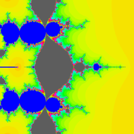
(a) A component of ${\mathcal{S}}_{4}^{{\mathbb{R}}+}$

(b) A component of ${\mathcal{S}}_{4}^{{\mathbb{R}}-}$

Figure 13: Examples of ${\mathfrak{C}}^{\pm}$ invariant components of Type B. In Case (a), the associated component of ${\mathcal{S}}_{4}^{{\mathbb{R}}+}$ is a horizontal line leading from the $\overline{1000}$t ideal point on the left to the $\overline{1010}$ ideal point which is off-screen on the right. (There is a slit to the left, since the $\overline{1000}$t escape region is locally a 3-fold branched covering of the $t$-parameter plane.) In Case (b), the associated component of ${\mathcal{S}}_{4}^{{\mathbb{R}}-}$ is a vertical line leading from the $\overline{0010}$ point below to the $\overline{0110}$ point above. $($These pictures are centered at $\,(a,v)~{}=(-.79263,\,1.19929)$ and $(a,v)~{}=~{}(0.743709\,i,\,0.029712\,i)$ respectively. $)$

Each component of Type B can be conveniently labelled by its Hubbard tree, together with a specification of the marked critical point $+a$ and the free critical point $-a$. This tree can be described as a piecewise linear map $~{}{\mathbf{f}}~{}$ from the interval $[0,\,p-1]$ to itself which takes integers to integers and is linear on each subinterval $[j,\,j+1]$. It will be convenient to extend $~{}{\mathbf{f}}~{}$ to a piecewise linear map from ${\mathbb{R}}$ to itself which has constant slope $>1$ outside of the interval $[0,\,p-1]$ in the ${\mathfrak{C}}^{+}$ invariant case, or constant slope $<-1$ in the ${\mathfrak{C}}^{-}$ invariant case. A map $~{}{\mathbf{f}}~{}$ of this type corresponds to a pair of components of Type B if and only if:

• ${\mathbf{f}}$ permutes the integers $\{0,\,1,\,\ldots,\,p-1\}$ cyclically, and

• ${\mathbf{f}}$ is  bimodal , i.e., with one local minimum and one local maximum.

To specify a unique component of Type B, we must also specify which of the two local extrema is to be the marked critical point. Let ${\bf a}_{0}$ be the marked critical point of ${\mathbf{f}}$ (or in other words the integer corresponding to $a_{0}$), and let $\widehat{\bf a}_{0}$ be the free critical point for ${\mathbf{f}}$. We will also use the notations ${\bf a}_{j}={\mathbf{f}}^{\circ j}({\bf a}_{0})$ and $\widehat{\bf a}_{j}={\mathbf{f}}^{\circ j}(\widehat{\bf a}_{0})$.

(a) with   $\widehat{\bf a}_{0}={\bf a}_{2}$

(b) with   ${\bf a}_{2}<\widehat{\bf a}_{0}$

Figure 14:

As an example, Figure 14(a) shows the graph for a typical Type B center in ${\mathcal{S}}_{5}^{{\mathbb{R}}+}$. The marked critical orbit is labelled as ${\bf a}_{0}\mapsto{\bf a}_{1}\mapsto\cdots\mapsto{\bf a}_{p-1}$, and the free critical point is labelled by a vertical dotted line. The information in this graph can be summarized by the inequalities

$${\bf a}_{1}<{\bf a}_{2}=\widehat{\bf a}_{0}<{\bf a}_{4}<{\bf a}_{0}<{\bf a}_{3}\,.$$

(Since this example is ${\mathfrak{C}}^{+}$ invariant, this is completely equivalent to the set of inequalities $a_{1}<a_{2}=\widehat{a}_{0}<a_{4}<a_{0}<a_{3}$.   In the ${\mathfrak{C}}^{-}$ invariant case, with the $a_{j}$ pure imaginary, we would write corresponding inequalities for the real numbers $a_{j}/i$.)

Definition. The  kneading sequence  associated with such a bimodal map with periodic marked critical point is a sequence of $p$ symbols which can be defined as follows. The free critical point $\widehat{\bf a}_{0}$ divides the real line into two halves. Assign the address 0 to every number on the same side as the marked critical point ${\bf a}_{0}$, and 1 to every point on the opposite side. (As an example, in Figures 14(a) and 14(b), everything to the right of the dotted line has address 0, and everything to the left has address 1.) Furthermore, define the address of the point $\widehat{\bf a}_{0}$ itself to be the symbol ★. The kneading sequence is then defined to be the sequence of addresses of the orbit points ${\bf a}_{1},\,{\bf a}_{2},\,\ldots,\,{\bf a}_{p}$ (where ${\bf a}_{p}={\bf a}_{0}$). Thus for a generic map, with $\widehat{\bf a}_{0}$ disjoint from the marked critical orbit, we obtain a sequence of zeros and ones. However, for the center point of any component of Type B (or in degenerate cases of Type A), the sequence will contain exactly one ★.

As an example, for Figure 14(a) the kneading sequence is 1★000. However, if we move the free critical point and the free critical value a little to the right, as indicated in Figure 14(b), leaving the rest of the graph unchanged, then the ordering becomes

$${\bf a}_{1}<{\bf a}_{2}<\widehat{\bf a}_{0}<{\bf a}_{4}<{\bf a}_{0}<{\bf a}_{3}\,,$$

and the kneading sequence will change to 11000, replacing ★ with 1. Similarly, if we move the free critical point a little to the left (still moving the free critical value to the right), we can replace ★ with 0. A similar argument applies to any component of Type B which is $~{}{\mathfrak{C}}^{\pm}$-invariant.

  

Figure 15: Graphs illustrating the transition from kneading sequence 1000 through  10★0  to  1010.

As a period 4 example, the relevant kneading sequences as we move from left to right near the middle of Figure 13(a) are illustrated in Figure 15.

The proof of Theorem 9.1 will depend on three lemmas.

Lemma 9.2 (Heckman).

No connected component of ${\mathcal{S}}_{p}^{{\mathbb{R}}\pm}$ can be a simple closed curve.

The proof is quite difficult. See [He].∎

    

Figure 16: Graphs of maps on the boundary of the connectedness locus within ${\mathcal{S}}_{p}^{{\mathbb{R}}+}~{}$ respectively $~{}{\mathcal{S}}_{p}^{{\mathbb{R}}-}$.

Lemma 9.3 (Milnor and Tresser).

Each connected component of ${\mathcal{S}}_{p}^{{\mathbb{R}}\pm}$ intersected with the connectedness locus is homeomorphic to a non-degenerate closed interval of real numbers. The two endpoints of this interval can be characterized as those maps in the interval for which the free critical value $~{}F(-a)~{}$ is an extreme point of the real or pure imaginary filled Julia set $($which is itself a closed interval—compare Figure 16$)$. It follows that this free critical value is a fixed point in the ${\mathfrak{C}}^{+}$-invariant case, and a period two point in the ${\mathfrak{C}}^{-}$-invariant case.

Proof. See [MTr, Lemma 7.2]. (The proof makes use of Lemma 9.2.)∎

Lemma 9.4.

For $~{}p>1~{}$ no two maps belonging to the same connected component of $~{}{\mathcal{S}}_{p}^{{\mathbb{R}}\pm}~{}$ can be conformally conjugate to each other. It follows that the connected components $P\subset{\mathcal{S}}_{p}^{{\mathbb{R}}\pm}$ occur in pairs, with each $P$ disjoint from ${\mathcal{I}}(P)$.

Proof. Note that two monic centered cubic polynomial maps are conformally conjugate if and only if they are either equal to each other, or carried one to the other by the involution ${\mathcal{I}}$. But if ${\mathcal{I}}$ interchanged two points in the same component $P$, then it would map $P$ onto itself, with a fixed point in the middle. This is impossible for $p>1$, since the only fixed point of $~{}{\mathcal{I}}(F_{a,v})=F_{-a,\,-v}$is the point $F_{0,0}\in{\mathcal{S}}_{1}$.∎

Proof of Theorem 9.1. If we use the canonical local parameter $t$, then the involution ${\mathfrak{C}}^{\pm}$ will transform $~{}t~{}$ to $~{}\pm\overline{t}+({\rm constant})$.  Hence the invariant curve ${\mathcal{S}}_{p}^{{\mathbb{R}}+}$ is represented by a horizontal line $\Im(t)={\rm constant}$, while ${\mathcal{S}}_{p}^{{\mathbb{R}}-}$ is represented by a vertical line $\Re(t)={\rm constant}$. (Compare Figure 13.) Clearly such a line can not have any limit point within the open surface ${\mathcal{S}}_{p}$. Since the connected component cannot be a simple closed curve, it can only be an infinite path $P$ which leads from one ideal point to another. We will see that these two ideal points must always be distinct when $p>1$, since they have different kneading invariants.

We next show that each component $P\subset{\mathcal{S}}_{p}^{{\mathbb{R}}\pm}$ contains at least one Type A or B center, that is, at least one map for which the free critical point $~{}\widehat{a}_{0}$ is equal to some point $~{}a_{j}~{}$ on the marked critical orbit. Otherwise, if the points $~{}a_{0},\,\ldots,\,a_{p-1}~{}$ and $~{}\widehat{a}_{0}~{}$ were pairwise distinct for all maps $~{}F\in P$,  then their ordering would be the same for all $~{}F\in P$.

We know that the left hand end of $P$ is contained in some escape component ${\mathcal{E}}_{1}$, and that the right hand end is contained in some escape component ${\mathcal{E}}_{2}$. Each of these components must map to itself under ${\mathfrak{C}}^{\pm}$. It follows from Lemma 3.1 that each escape region is conformally diffeomorphic to ${\mathbb{C}}{\smallsetminus}\overline{\mathbb{D}}$. Furthermore, if the escape region is ${\mathfrak{C}}^{\pm}$-invariant, then we can choose this conformal diffeomorphism so that ${\mathfrak{C}}^{\pm}$ corresponds to the involution $~{}z\mapsto\pm\overline{z}$ of ${\mathbb{C}}{\smallsetminus}\overline{\mathbb{D}}$.  Thus the fixed point set will correspond to the real axis in the ${\mathfrak{C}}^{+}$ case, or the imaginary axis in the ${\mathfrak{C}}^{-}$ case. It follows that the intersection ${\mathcal{E}}_{h}\cap P$ is always a path leading from the ideal point to some boundary point of ${\mathcal{E}}_{h}$. It then follows from Lemma 9.3 that the remaining portion of $P$, its intersection with the connectedness locus, is a closed interval of real numbers, bounded by two post-critically finite maps. Hence each of these boundary maps is uniquely determined, up to conjugacy, by its Hubbard tree. If there were no center points of Type A or B within this path $P$, then the two endpoints of $P$ intersected with the connectness locus would have to have isomorphic Hubbard trees. But this is impossible by Lemma 9.4; hence $P$ must contain a Type A or B center.

Finally, we must prove that there cannot be two such Type A or B centers on the path $P$. Otherwise, as $F$ varies over the subinterval $P^{\prime}$ joining two consecutive centers, the $p+1$ points $~{}a_{0},\,a_{1},\,\ldots,\,a_{p-1}~{}$ and $\widehat{a}_{0}$ would vary smoothly and remain distinct. But, among all possible variations, there is only one way of converging to a Type A or B center. Suppose for example that one of the endpoints of $P^{\prime}$ is topologically conjugate to the map of Figure 14(a), and suppose as in Figure 14(b) that we have $a_{1}<a_{2}<\widehat{a}_{0}<a<a_{4}<a_{0}<a_{3}$ for the points $F\in P^{\prime}$. Since only one of the two endpoints of the interval $[a_{2},\,a_{4}]$ is a local maximum, we can converge to a Type B center only by letting $\widehat{a}_{0}$ converge to $a_{2}$. This shows that the two endpoints of the interval $P^{\prime}$ must have the same Hubbard tree. But this is impossible by Lemma 9.4. The argument in the general case is completely analogous.

Finally, it follows from the discussion of Figures 14(a) and 14(b) that the two endpoints of the path $P$ must be ideal points with kneading sequences which differ in exactly one entry. Hence these two endpoints are certainly distinct.$\quad\square$

Corollary 9.5.

A connected component in ${\mathcal{S}}_{p}^{{\mathbb{R}}\pm}$ is uniquely determined by the ordering of the points ${\bf a}_{0},\,{\bf a}_{1},\,\ldots,\,{\bf a}_{p-1}$ in the marked critical orbit.

The proof is immediate. If the graph associated with this ordering has an interior local maximum or minimum at a point ${\bf a}_{j}$ with $j\neq 0$, then we must set $~{}\widehat{\bf a}_{0}={\bf a}_{j}$.  Otherwise, $\widehat{\bf a}_{0}$ must be one of the two endpoints, and only one of the two is compatible with ${\mathfrak{C}}^{\pm}$ invariance. In either case, the Hubbard tree and hence the associated Type B component is uniquely determined.$\quad\square$

Remark 9.6.

Notice in Figure 13(a) [and 13(b)] that there is also a small component of Type D on the real [or imaginary] axis, immediately to the left [or below] the big component. In fact, for periods $p\geq 3$, every ${\mathfrak{C}}^{\pm}$-invariant Type B component is associated with a ${\mathfrak{C}}^{\pm}$-invariant Type D component which is immediately adjacent to it, consisting of maps for which both attracting orbits have period $p$. The common boundary point is a parabolic map, with parabolic orbit of period $p$ on the boundary of the cycle of attracting Fatou components. (Compare [MTr, Lemma 7.1].)

The associated Hubbard tree (or graph) can easily be constructed from the piecewise linear map $~{}f~{}$ for the Type B center. Suppose for example, as in Figure 14(a), that $f$ has a local maximum $\widehat{\bf a}_{1}=f(\widehat{\bf a}_{0})$ at the free critical point. Consider a one parameter family of modified piecewise linear functions, as in Figure 14(b), as follows. Choose some small $\epsilon>0$, and replace the original free critical point $\widehat{\bf a}_{0}={\bf a}_{k}$ by $~{}\widehat{\bf a}_{0}={\bf a}_{k}\pm\epsilon\,$;  but set the free critical value $f_{t}(\widehat{\bf a}_{0})$ equal to $f({\bf a}_{k})+t={\bf a}_{k+1}+t$ for small $t>0$, leaving all of the marked orbit points ${\bf a}_{j}$ unchanged. Then as $t$ increases, for each $j\leq p$ the forward image $f_{t}^{\circ j}(\widehat{\bf a}_{0})$ will move linearly to the left or right. Choose the sign in the equation $\widehat{\bf a}_{0}={\bf a}_{k}\pm\epsilon$ so that $f_{t}^{\circ p}(\widehat{a}_{0})$ will move towards $\widehat{\bf a}_{0}$. For some first value $t_{0}$, we must have the precise equality $f_{t_{0}}^{\circ p}(\widehat{\bf a}_{0})=\widehat{\bf a}_{0}$. Then $f_{t_{0}}$ represents the required Type D center, with both periodic orbits periodic of period $p$.

Araceli Bonifant; Mathematics Department, University of Rhode Island, Kingston, R.I., 02881. e-mail: bonifant@math.uri.edu

Jan Kiwi; Facultad de Matemáticas, Pontificia Universidad Católica, Casilla 306, Correo 22, Santiago de Chile, Chile. e-mail: jkiwi@puc.cl

John Milnor; Institute for Mathematical Sciences, Stony Brook University, Stony Brook, NY. 11794-3660. e-mail: jack@math.sunysb.edu

References

- [AC] D. A. Aruliah and R. M. Corless, Numerical parameterization of affine varieties using ODE’s, International Conference on Symbolic and Algebraic Computation. Proceedings 2004 International Symposium on Symbolic and Algebraic Computation, Santander, Spain, 2004, 12–18.
- [Br] B. Branner, Cubic polynomials, turning around the connectedness locus, pp. 391–427 of “Topological Methods in Mathematics” (edit. Goldberg and Phillips), Publish or Perish, 1993.
- [BM] A. Bonifant and J. Milnor, Cubic polynomial maps with periodic critical orbit, Part III: External rays, in preparation.
- [BH] B. Branner and J. H. Hubbard, The iteration of cubic polynomials II, patterns and parapatterns, Acta Math. 169 (1992) 229–325.
- [DMS] L. DeMarco and A. Schiff, Enumerating the basins of infinity for cubic polynomials. To appear, Special Volume of Journal of Difference Equations and Applications.
- [H] D. Harris, Turning curves for critically recurrent cubic polynomials, Nonlinearity 12 2 (1999), 411–418.
- [He] C. Heckman, Monotonicity and the construction of quasiconformal conjugacies in the real cubic family, Thesis, Stony Brook 1996.
- [IK] H. Inou and J. Kiwi, Combinatorics and topology of straightening maps I: compactness and bijectivity, ArXiv:0809.1262.
- [IKR] H. Inou, J. Kiwi and P. Roesch, work in preparation.
- [K1] J. Kiwi, Puiseux series polynomial dynamics and iteration of complex cubic polynomials, Ann. Inst. Fourier (Grenoble) 56 (2006) 1337–1404.
- [K2] J. Kiwi, manuscript in preparation.
- [M] J. Milnor, Cubic Polynomial Maps with Periodic Critical Orbit, Part I, In: “Complex Dynamics Families and Friends”, ed. D. Schleicher, A. K. Peters 2009, pp. 333-411.
- [MTr] ——— and C. Tresser, On entropy and monotonicity for real cubic maps, Comm. Math. Phys. 209 (2000) 123-178.
- [MTh] ——– and W. Thurston, On iterated maps of the interval, In: “Dynamical systems”, Alexander, J.C. (ed.). Lecture Notes in Mathematics N1342. Berlin: Springer, 1988, pp. 465-563.
- [R] J. Rivera-Letelier, Dynamique des fonctions rationnelles sur des corps locaux, Geometric methods in dynamics. II. Astérisque No. 287 (2003), xv, 147–230.