The Intersection of Two Halfspaces Has
High Threshold Degree

Abstract

The threshold degree of a Boolean function $f\colon\{0,1\}^{n}\to\{-1,+1\}$ is the least degree of a real polynomial $p$ such that $f(x)\equiv\operatorname{sgn}p(x).$ We construct two halfspaces on $\{0,1\}^{n}$ whose intersection has threshold degree $\Theta(\sqrt{n}),$ an exponential improvement on previous lower bounds. This solves an open problem due to Klivans (2002) and rules out the use of perceptron-based techniques for PAC learning the intersection of two halfspaces, a central unresolved challenge in computational learning. We also prove that the intersection of two majority functions has threshold degree $\Omega(\log n),$ which is tight and settles a conjecture of O’Donnell and Servedio (2003).

Our proof consists of two parts. First, we show that for any nonconstant Boolean functions $f$ and $g,$ the intersection $f(x)\wedge g(y)$ has threshold degree $O(d)$ if and only if $\|f-F\|_{\infty}+\|g-G\|_{\infty}<1$ for some rational functions $F,$ $G$ of degree $O(d).$ Second, we settle the least degree required for approximating a halfspace and a majority function to any given accuracy by rational functions.

Our technique further allows us to make progress on Aaronson’s challenge (2008) and contribute strong direct product theorems for polynomial representations of composed Boolean functions of the form $F(f_{1},...,f_{n}).$ In particular, we give an improved lower bound on the approximate degree of the AND-OR tree.

1 Introduction

Representations of Boolean functions by real polynomials play an important role in theoretical computer science, with applications ranging from complexity theory to quantum computing and learning theory. The surveys in [7, 40, 13, 43] offer a glimpse into the diversity of these results and techniques. We study one such representation scheme known as sign-representation. Specifically, fix a Boolean function $f\colon X\to\{-1,+1\}$ for some finite set $X\subset\mathbb{R}^{n},$ such as the hypercube $X=\{-1,+1\}^{n}.$ The threshold degree of $f,$ denoted $\operatorname{deg_{\pm}}(f),$ is the least degree of a polynomial $p(x_{1},\dots,x_{n})$ such that

$$f(x)=\operatorname{sgn}p(x)$$

for each $x\in X.$ In other words, the threshold degree of $f$ is the least degree of a real polynomial that represents $f$ in sign.

The formal study of this complexity measure and of sign-representations in general began in 1969 with the seminal work of Minsky and Papert [30], who examined the threshold degree of several common functions. Since then, sign-representations have found a variety of applications in theoretical computer science. Paturi and Saks [35] and later Siu et al. [47] used Boolean functions with high threshold degree to obtain size-depth trade-offs for threshold circuits. The well-known result, due to Beigel et al. [9], that $\mathsf{PP}$ is closed under intersection is also naturally interpreted in terms of threshold degree. In another development, Aspnes et al. [6] used the notion of threshold degree and its relaxations to obtain oracle separations for $\mathsf{PP}$ and to give an insightful new proof of classical lower bounds for $\mathsf{AC}^{0}.$ Krause and Pudlák [26, 27] used random restrictions to show that the threshold degree gives lower bounds on the weight and density of perceptrons and their generalizations, which are well-studied computational models.

Learning theory is another area in which the threshold degree of Boolean functions is of considerable interest. Specifically, functions with low threshold degree can be efficiently PAC learned under arbitrary distributions via linear programming. The current fastest algorithm for PAC learning polynomial-size DNF formulas, due to Klivans and Servedio [21], is an illustrative example: it is based precisely on an upper bound on the threshold degree of this concept class.

The threshold degree has recently become a versatile tool in communication complexity. The starting point in this line of work is the Degree/Discrepancy Theorem [41, 42], which states that any Boolean function with high threshold degree induces a communication problem with low discrepancy and thus high communication complexity in almost all models. This result was used in [41] to show the optimality of Allender’s simulation of $\mathsf{AC}^{0}$ by majority circuits [4], thus solving an open problem of Krause and Pudlák [26]. Known lower bounds on the threshold degree have played an important role in recent progress [44, 38] on unbounded-error communication complexity, which is considerably more powerful than the models above.

In summary, the threshold degree has a variety of applications in circuit complexity, learning theory, and communication complexity. Nevertheless, analyzing the threshold degree has remained a difficult task, and Minsky and Papert’s symmetrization technique from 1969 has been essentially the only method available. Unfortunately, symmetrization only applies to symmetric Boolean functions and certain derivations thereof. In a recent tutorial presented at the FOCS’08 conference, Aaronson [2] re-posed the challenge of developing new analytic techniques for multivariate real polynomials that represent Boolean functions. We make significant progress on this challenge in the context of sign-representation, contributing a number of strong direct product theorems for the threshold degree. As an application, we construct two halfspaces on $\{0,1\}^{n}$ whose intersection has threshold degree $\Omega(\sqrt{n}),$ which solves an open problem due to Klivans [19] and rules out the use of perceptron-based techniques for PAC learning the intersection of even two halfspaces (a central unresolved challenge in computational learning theory). We give a detailed description of our results in Sections 1.1–1.3, followed by a discussion of our techniques in Section 1.4.

1.1 Results for general compositions

Our first result is a general direct product theorem for the threshold degree of composed functions.

Theorem 1.1 (Threshold degree).

Consider functions $f\colon X\to\{-1,+1\}$ and $F\colon\{-1,+1\}^{k}\to\{-1,+1\},$ where $X\subset\mathbb{R}^{n}$ is a finite set. Then

$$\operatorname{deg_{\pm}}(F(f,\dots,f))\geqslant\operatorname{deg_{\pm}}(F)\operatorname{deg_{\pm}}(f).$$

Theorem 1.1 gives the best possible lower bound that depends on $\operatorname{deg_{\pm}}(F)$ and $\operatorname{deg_{\pm}}(f)$ alone. In particular, the bound is tight whenever $F=\text{\rm PARITY}$ or $f=\text{\rm PARITY}.$ To our knowledge, the only previous direct product theorem of any kind for the threshold degree was the XOR lemma in [33], which states that the XOR of $k$ copies of a given function $f\colon X\to\{-1,+1\}$ has threshold degree $k\operatorname{deg_{\pm}}(f).$

We are able to generalize Theorem 1.1 to the notion of $\epsilon$-approximate degree $\operatorname{\deg_{\epsilon}}(F),$ which is the least degree of a real polynomial $p$ with $\|F-p\|_{\infty}\leqslant\epsilon.$ This notion plays a fundamental role in complexity theory, learning theory, and quantum computing and was also re-posed as an analytic challenge in Aaronson’s tutorial [2]. We have:

Theorem 1.2 (Approximate degree).

Fix functions $f\colon X\to\{-1,+1\}$ and $F\colon\{-1,+1\}^{k}\to\{-1,+1\},$ where $X\subset\mathbb{R}^{n}$ is a finite set. Then for $0<\epsilon<1,$

$$\deg_{\epsilon}(F(f,\dots,f))\geqslant\deg_{\epsilon}(F)\operatorname{deg_{\pm}}(f).$$

Again, Theorem 1.2 gives the best lower bound that depends on $\deg_{\epsilon}(F)$ and $\operatorname{deg_{\pm}}(f)$ alone. For example, the stated bound is tight for any function $F$ when $f=\text{\rm PARITY}.$ In Section 3.1, we prove various other results involving bounded-error and small-bias approximation, as well as compositions of the form $F(f_{1},\dots,f_{k})$ where $f_{1},\dots,f_{k}$ may all be distinct.

We use Theorem 1.2 to obtain an improved lower bound on the approximate degree of the well-studied AND-OR tree, given by

$$f(x)=\bigvee_{i=1}^{n}\bigwedge_{j=1}^{n}x_{ij}.$$ (1.1)

Prior to this work, the best lower bound was $\Omega(n^{0.66\dots}),$ due to Ambainis [5]. Preceding it were lower bounds of $\Omega(\sqrt{n})$ due to Nisan and Szegedy [32] and $\Omega(\sqrt{n\log n})$ due to Shi [46]. We improve the standing lower bound from $\Omega(n^{0.66\dots})$ to $\Omega(n^{0.75}),$ the best upper bound being $O(n)$ due to Høyer et al. [16].

Theorem 1.3 (AND-OR Tree).

Define $f\colon\{-1,+1\}^{n^{2}}\to\{-1,+1\}$ by (1.1). Then

$$\deg_{1/3}(f)=\Omega(n^{0.75}).$$

Furthermore, the proof of Theorem 1.3 is simpler and more modular than the previous lower bound [5], which was based on the collision and element distinctness problems.

1.2 Results for specific compositions

While Theorems 1.1 and 1.2 give the best lower bounds that depend on $\operatorname{deg_{\pm}}(F),$ $\operatorname{deg_{\pm}}(f),$ and $\operatorname{\deg_{\epsilon}}(F)$ alone, much stronger lower bounds can be derived in some cases by exploiting additional structure of $F$ and $f.$ Consider the special but illustrative case of the conjunction of two functions. In other words, we are given functions $f\colon X\to\{-1,+1\}$ and $g\colon Y\to\{-1,+1\}$ for some finite sets $X,Y\subset\mathbb{R}^{n}$ and would like to determine the threshold degree of their conjunction, $(f\wedge g)(x,y)=f(x)\wedge g(y).$ A simple and elegant method for sign-representing $f\wedge g,$ due to Beigel et al. [9], is to use rational approximation. Specifically, let $p_{1}(x)/q_{1}(x)$ and $p_{2}(y)/q_{2}(y)$ be rational functions of degree $d$ that approximate $f$ and $g,$ respectively, in the following sense:

$$\max_{x\in X}\left|f(x)-\frac{p_{1}(x)}{q_{1}(x)}\right|\,+\,\max_{y\in Y}\left|g(y)-\frac{p_{2}(y)}{q_{2}(y)}\right|\,<\,1.$$ (1.2)

Letting $-1$ and $+1$ correspond to “true” and “false,” respectively, we obtain:

$$f(x)\wedge g(y) \equiv\operatorname{sgn}\{1+f(x)+g(y)\}\rule{0.0pt}{19.91692pt}\equiv\operatorname{sgn}\left\{1+\frac{p_{1}(x)}{q_{1}(x)}+\frac{p_{2}(y)}{q_{2}(y)}\right\}.$$ (1.3)

Multiplying the last expression in braces by the positive quantity $q_{1}(x)^{2}q_{2}(y)^{2}$ gives

$$\quad f(x)\wedge g(y)\equiv\operatorname{sgn}\left\{q_{1}(x)^{2}q_{2}(y)^{2}\right.\\ \left.+p_{1}(x)q_{1}(x)q_{2}(y)^{2}+p_{2}(y)q_{1}(x)^{2}q_{2}(y)\right\},\quad$$

whence $\operatorname{deg_{\pm}}(f\wedge g)\leqslant 4d.$ In summary, if $f$ and $g$ can be approximated as in (1.2) by rational functions of degree at most $d,$ then the conjunction $f\wedge g$ has threshold degree at most $4d.$

It is natural to ask whether there exists a better construction. After all, given a sign-representing polynomial $p(x,y)$ for $f(x)\wedge g(y),$ there is no reason to expect that $p$ arises from the sum of two independent rational functions as in (1.3). Indeed, $x$ and $y$ can be tightly coupled inside $p(x,y)$ and can interact in complicated ways. Our next result is that, surprisingly, no such interactions can beat the simple construction above. In other words, the sign-representation based on rational functions always achieves the optimal degree, up to a small constant factor.

Theorem 1.4 (Conjunctions of functions).

Let $f\colon X\to\{-1,+1\}$ and $g\colon Y\to\{-1,+1\}$ be given functions, where $X,Y\subset\mathbb{R}^{n}$ are arbitrary finite sets. Assume that $f$ and $g$ are not identically false. Let $d=\operatorname{deg_{\pm}}(f\wedge g).$ Then there exist degree-$4d$ rational functions

$$\frac{p_{1}(x)}{q_{1}(x)},\quad\frac{p_{2}(y)}{q_{2}(y)}$$

that satisfy (1.2).

Via repeated applications of Theorem 1.4, we are able to obtain analogous results for conjunctions $f_{1}\wedge f_{2}\wedge\cdots\wedge f_{k}$ for any Boolean functions $f_{1},f_{2},\dots,f_{k}$ and any $k.$ Our results further extend to compositions $F(f_{1},\dots,f_{k})$ for various $F$ other than $F=\text{\rm AND},$ such as halfspaces and read-once AND/OR/NOT formulas. We defer a more detailed description of these extensions to Section 3.4, limiting this overview to the following representative special case.

Theorem 1.5 (Extension to multiple functions).

Let $f_{1},f_{2},\dots,f_{k}$ be nonconstant Boolean functions on finite sets $X_{1},X_{2},\dots,X_{k}\subset\mathbb{R}^{n},$ respectively. Let $F\colon\{-1,+1\}^{k}\to\{-1,+1\}$ be a halfspace or a read-once AND/OR/NOT formula. Assume that $F$ depends on all of its $k$ inputs and that the composition $F(f_{1},f_{2},\dots,f_{k})$ has threshold degree $d.$ Then there is a degree-$D$ rational function $p_{i}/q_{i}$ on $X_{i},$ $i=1,2,\dots,k,$ such that

$$\sum_{i=1}^{k}\;\max_{x_{i}\in X_{i}}\left|f_{i}(x_{i})-\frac{p_{i}(x_{i})}{q_{i}(x_{i})}\right|<1,$$

where $D=8d\log 2k.$

Theorem 1.5 is close to optimal. For example, when $F=\text{\rm AND},$ the upper bound on $D$ is tight up to a factor of $\Theta(k\log k)$; for all $F$ in the statement of the theorem, it is tight up to a polynomial in $k.$ See Remark 3.22 for details.

Theorems 1.4 and 1.5 contribute a strong technique for proving lower bounds on the threshold degree, via rational approximation. Prior to this paper, it was a substantial challenge to analyze the threshold degree even for compositions of the form $f\wedge g.$ Indeed, we are only aware of the work in [30, 33], where the threshold degree of $f\wedge g$ was studied for the special case $f=g=\text{\sc majority}.$ The main difficulty in those previous works was analyzing the unintuitive interactions between $f$ and $g.$ Our results remove this difficulty, even in the general setting of compositions $F(f_{1},f_{2},\dots,f_{k})$ for arbitrary $f_{1},f_{2},\dots,f_{k}$ and various combining functions $F.$ Specifically, Theorems 1.4 and 1.5 make it possible to study the base functions $f_{1},f_{2},\dots,f_{k}$ individually, in isolation. Once their rational approximability is understood, one immediately obtains lower bounds on the threshold degree of $F(f_{1},f_{2},\dots,f_{k}).$

1.3 Results for intersections of two halfspaces

As an application of our direct product theorems in Section 1.2, we obtain the first strong lower bounds on the threshold degree of intersections of halfspaces, i.e., intersections of functions of the form $f(x)=\operatorname{sgn}(\sum\alpha_{i}x_{i}-\theta)$ for some reals $\alpha_{1},\dots,\alpha_{n},\theta.$ In light of Theorem 1.4, this task amounts to proving that rational functions of low degree cannot approximate a given halfspace. We accomplish this in the following theorem, where the notation $\operatorname{rdeg}_{\epsilon}(f)$ stands for the least degree of a rational function $A$ with $\|f-A\|_{\infty}\leqslant\epsilon.$

Theorem 1.6 (Approximation of a halfspace).

Let $f\colon\{-1,+1\}^{n^{2}}\to\{-1,+1\}$ be given by

$$f(x)=\operatorname{sgn}\left(1+\sum_{i=1}^{\phantom{A}n\phantom{A}}\sum_{j=1}^{n}2^{i}x_{ij}\right).$$ (1.4)

Then for $1/3<\epsilon<1,$

$$\operatorname{rdeg}_{\epsilon}(f)=\Theta\left(1+\frac{\phantom{A}n\phantom{A}}{\log\{1/(1-\epsilon)\}}\right).$$

Furthermore, for all $\epsilon>0,$

$$\operatorname{rdeg}_{\epsilon}(f)\leqslant 64n\lceil\log_{2}n\rceil+1.$$

The function (1.4) is known as the canonical halfspace. Thus, Theorem 1.6 shows that a rational function of degree $\Theta(n)$ is necessary and sufficient for approximating the canonical halfspace within $1/3.$ The upper bound in this theorem follows readily from classical work by Newman [31], and it is the lower bound that has required of us technical novelty and effort. The best previous degree lower bound for constant-error approximation for any halfspace was $\Omega(\log n/\log\log n),$ obtained implicitly in [33]. We complement Theorem 1.6 with a full solution for another common halfspace, the majority function.

Theorem 1.7 (Approximation of majority).

Let $\text{\rm MAJ}_{n}\colon\{-1,+1\}^{n}\to\{-1,+1\}$ denote the majority function. Then

$$\operatorname{rdeg}_{\epsilon}(\text{\rm MAJ}_{n})=\begin{cases}\displaystyle\Theta\left(\log\left\{\frac{2n}{\log(1/\epsilon)}\right\}\cdot\log\frac{1}{\epsilon}\right),&\qquad 2^{-n}<\epsilon<1/3,\\ \rule{0.0pt}{28.45274pt}\displaystyle\Theta\left(1+\frac{\log n}{\log\{1/(1-\epsilon)\}}\right),&\qquad 1/3\leqslant\epsilon<1.\end{cases}$$

Again, the upper bound in Theorem 1.7 is relatively straightforward. Indeed, an upper bound of $O(\log\{1/\epsilon\}\log n)$ for $0<\epsilon<1/3$ was known and used in the complexity literature long before our work [35, 47, 9, 20], and we only somewhat tighten that upper bound and extend it to all $\epsilon.$ Our primary contribution in Theorem 1.7, then, is a matching lower bound on the degree, which requires considerable effort. The closest previous line of research concerns continuous approximation of the sign function on $[-1,-\epsilon]\cup[\epsilon,1],$ which unfortunately gives no insight into the discrete case. For example, the lower bound derived by Newman [31] in the continuous setting is based on the integration of relevant rational functions with respect to a suitable weight function, which has no meaningful discrete analogue. We discuss our solution in greater detail at the end of the introduction.

Our first application of these lower bounds for rational approximation is to construct an intersection of two halfspaces with high threshold degree. In what follows, the symbol $f\wedge f$ denotes the conjunction of two independent copies of a given function $f.$

Theorem 1.8 (Intersection of two halfspaces).

Let $f\colon\{-1,+1\}^{n^{2}}\to\{-1,+1\}$ be given by (1.4). Then

$$\operatorname{deg_{\pm}}(f\wedge f)=\Omega(n).$$

The lower bound in Theorem 1.8 is tight and matches the construction by Beigel et al. [9]. Prior to our work, only an $\Omega(\log n/\log\log n)$ lower bound was known on the threshold degree of the intersection of two halfspaces, due to O’Donnell and Servedio [33], preceded in turn by an $\omega(1)$ lower bound of Minsky and Papert [30]. Note that Theorem 1.8 requires the difficult part of Theorem 1.6, namely, the lower bound for the rational approximation of a halfspace.

Theorem 1.8 solves an open problem in computational learning theory, due to Klivans [19]. In more detail, recall that Boolean functions with low threshold degree can be efficiently PAC learned under arbitrary distributions, by expressing an unknown function as a perceptron with unknown weights and solving the associated linear program [21, 20]. Now, a central challenge in the area is PAC learning the intersection of two halfspaces under arbitrary distributions, which remains unresolved despite much effort and solutions to some restrictions of the problem, e.g., [28, 48, 20, 23]. Prior to this paper, it was unknown whether intersections of two halfspaces on $\{0,1\}^{n}$ are amenable to learning via perceptron-based techniques. Specifically, Klivans [19, §7] asked for a lower bound of $\Omega(\log n)$ or better on the threshold degree of the intersection of two halfspaces. We solve this problem with a lower bound of $\Omega(\sqrt{n}),$ thereby ruling out the use of perceptron-based techniques for learning the intersection of two halfspaces in subexponential time. To our knowledge, Theorem 1.8 is the first unconditional, structural lower bound for PAC learning the intersection of two halfspaces; all previous hardness results for the problem were based on complexity-theoretic assumptions [10, 3, 25, 18]. We complement Theorem 1.8 as follows.

Theorem 1.9 (Mixed intersection).

Let $f\colon\{-1,+1\}^{n^{2}}\to\{-1,+1\}$ be given by (1.4). Let $g\colon\{-1,+1\}^{\lceil\sqrt{n}\rceil}\to\{-1,+1\}$ be the majority function. Then

$$\operatorname{deg_{\pm}}(f\wedge g)=\Theta(\sqrt{n}).$$

In words, even if one of the halfspaces in Theorem 1.8 is replaced by a majority function, the threshold degree will remain high, resulting in a challenging learning problem. Finally, we have:

Theorem 1.10 (Intersection of two majorities).

Consider the majority function $\text{\rm MAJ}_{n}\colon\{-1,+1\}^{n}\to\{-1,+1\}.$ Then

$$\operatorname{deg_{\pm}}(\text{\rm MAJ}_{n}\wedge\text{\rm MAJ}_{n})=\Omega(\log n).$$

Theorem 1.10 is tight, matching the construction of Beigel et al. [9]. It settles a conjecture of O’Donnell and Servedio [33], who gave a lower bound of $\Omega(\log n/\log\log n)$ with completely different techniques and conjectured that the true answer was $\Omega(\log n).$ Theorems 1.8–1.10 are of course also valid for disjunctions rather than conjunctions. Furthermore, Theorems 1.8 and 1.10 remain tight with respect to conjunctions of any constant number of functions.

Finally, we believe that the lower bounds for rational approximation in Theorems 1.6 and 1.7 are of independent interest. Rational functions are classical objects with various applications in theoretical computer science [9, 35, 47, 20, 1], and yet our ability to prove strong lower bounds for the rational approximation of Boolean functions has seen little progress since the seminal work in 1964 by Newman [31]. To illustrate some of the counterintuitive phenomena involved in rational approximation, consider the familiar function $\text{\rm OR}_{n}\colon\{0,1\}^{n}\to\{-1,+1\},$ given by $\text{\rm OR}_{n}(x)=1\Leftrightarrow x=0.$ A well-known result of Nisan and Szegedy [32] states that $\deg_{1/3}(f)=\Theta(\sqrt{n}),$ meaning that a polynomial of degree $\Theta(\sqrt{n})$ is required for approximation within $1/3.$ At the same time, we claim that $\operatorname{rdeg}_{\epsilon}(f)=1$ for all $0<\epsilon<1.$ Indeed, let

$$A_{M}(x)=\frac{1-M\sum x_{i}}{1+M\sum x_{i}}.$$

Then $\|f-A_{M}\|_{\infty}\to 0$ as $M\to\infty.$ This example illustrates that proving lower bounds for rational functions can be a difficult and unintuitive task. We hope that Theorems 1.6 and 1.7 in this paper will spur further progress on the rational approximation of Boolean functions.

1.4 Our techniques

We use one set of techniques to obtain our direct product theorems for the threshold degree (Sections 1.1 and 1.2) and another, unrelated set of techniques to analyze the rational approximation of halfspaces (Section 1.3). We will give a separate overview of the technical development in each case.

Direct product theorems. In symmetrization, one takes an assumed multivariate polynomial $p$ that sign-represents a given symmetric function and converts $p$ into a univariate polynomial, which is amenable to direct analysis. No such approach works for the function compositions of this paper, whose sign-representing polynomials can have complicated structure and will not simplify in a meaningful way. This leads us to pursue a completely different approach.

Specifically, our results are based on a thorough study of the linear programming dual of the sign-representation problems at hand. The challenge in our work is to bring out, through the dual representation, analytic properties that will obey a direct product theorem. Depending on the context (Theorem 1.1, 1.2, or 1.4), the property in question can be nonnegativity, correlation, orthogonality, certain quotient structure, or a combination of several of these. A strength of this approach is that it works with the sign-representation problem itself (over which we have considerable control) rather than an assumed sign-representing polynomial (whose structure we can no longer control in a meaningful way). We are confident that this approach will find other applications.

As a concrete illustration, we briefly describe the idea behind Theorem 1.4. The dual object with which we work there is a certain problem of finding, in the positive spans of two given matrices, two vectors whose corresponding entries have comparable magnitude. By an analytic argument, we are able to prove that this intermediate problem has the sought direct-product property, giving the missing link between sign-representation and rational approximation. Thus, by working with the dual, we implicitly decompose any sign-representation $p(x,y)$ of the function $f(x)\wedge g(y)$ into individual rational approximants for $f$ and $g,$ regardless of how tightly the $x$ and $y$ parts are coupled inside $p.$

Rational approximation. Our proof of Theorem 1.6 is built around two key ideas. The first is a new technique for placing lower bounds on the degree of a given polynomial $p\in\mathbb{R}[x_{1},x_{2},\dots,x_{n}]$ with prescribed approximate behavior, whereby one constructs a degree-nonincreasing linear map $M\colon\mathbb{R}[x_{1},x_{2},\dots,x_{n}]\to\mathbb{R}[x]$ and argues that $Mp$ has high degree. This technique is crucial to proving Theorem 1.6, which is not amenable to standard techniques such as symmetrization. As applied in this work, the technique amounts to constructing random variables $\mathbf{x}_{1},\mathbf{x}_{2},\dots,\mathbf{x}_{n}$ in Euclidean space that, on the one hand, satisfy the linear dependence $\sum 2^{i}\mathbf{x}_{i}\equiv\mathbf{z}$ for a suitably fixed vector $\mathbf{z}$ and, on the other hand, in expectation look independent to any low-degree polynomial $p\in\mathbb{R}[x_{1},x_{2},\dots,x_{n}].$ We pass, then, from $p$ to a univariate polynomial by observing that $\operatorname*{\mathbf{E}}[p(\mathbf{x}_{1},\dots,\mathbf{x}_{n})]=q(\mathbf{z})$ for some univariate polynomial $q$ of degree no greater than the degree of $p.$ This technique is a substantial departure from previous methods and shows promise on other problems involving approximation by polynomials or rational functions.

Second, we are able to prove that the rational approximation of the sign function has a self-reducibility property on the discrete domain. More specifically, we are able to give an explicit solution to the dual of the rational approximation problem by distributing the nodes as in known positive results. What makes this program possible in the first place is our ability to zero out the dual object on the complementary domain, which is where the above map $M\colon\mathbb{R}[x_{1},x_{2},\dots,x_{n}]\to\mathbb{R}[x]$ plays a crucial role. This dual approach, too, departs entirely from previous analyses. In particular, recall that Newman’s lower-bound analysis is specialized to the continuous domain and does not extend to the setting of Theorem 1.7, let alone Theorem 1.6.

Recent progress

A recent follow-up paper [45] proves that the intersection of two halfspaces on $\{0,1\}^{n}$ has threshold degree $\Theta(n),$ improving on the lower bound of $\Omega(\sqrt{n})$ in this work. We have also learned that the inequality $\deg_{\epsilon}(F(f,\dots,f))\geqslant\operatorname{\deg_{\epsilon}}(F)\operatorname{deg_{\pm}}(f)$ was derived independently by Lee [29] in a recent work on read-once Boolean formulas.

2 Preliminaries

Throughout this work, the symbol $t$ refers to a real variable, whereas $u,$ $v,$ $w,$ $x,$ $y,$ $z$ refer to vectors in $\mathbb{R}^{n}$ and in particular in $\{-1,+1\}^{n}.$ We adopt the following standard definition of the sign function:

$$\operatorname{sgn}t=\begin{cases}-1,&t<0,\\ 0,&t=0,\\ 1,&t>0.\end{cases}$$

We will also have occasion to use the following modified sign function:

$$\operatorname{\widetilde{sgn}}t=\begin{cases}-1,&t<0,\\ 1,&t\geqslant 0.\end{cases}$$

Equations and inequalities involving vectors in $\mathbb{R}^{n},$ such as $x<y$ or $x\geqslant 0,$ are to be interpreted component-wise, as usual.

Throughout this manuscript, we view Boolean functions as mappings $f\colon X\to\{-1,+1\}$ for some finite set $X,$ where $-1$ and $+1$ correspond to “true” and “false,” respectively. If $\mu_{1},\dots,\mu_{k}$ are probability distributions on finite sets $X_{1},\dots,X_{k},$ respectively, then $\mu_{1}\times\cdots\times\mu_{k}$ stands for the probability distribution on $X_{1}\times\cdots\times X_{k}$ given by

$$(\mu_{1}\times\cdots\times\mu_{k})(x_{1},\dots,x_{k})=\prod_{i=1}^{k}\mu_{i}(x_{i}).$$

The majority function on $n$ bits, $\text{\rm MAJ}_{n}\colon\{-1,+1\}^{n}\to\{-1,+1\},$ is given by

$$\text{\rm MAJ}_{n}(x)=\begin{cases}1,&\sum x_{i}>0,\\ -1,&\text{otherwise.}\end{cases}$$

The symbol $P_{k}$ stands for the family of all univariate real polynomials of degree up to $k.$ The following combinatorial identity is well-known.

Fact 2.1.

For every integer $n\geqslant 1$ and every polynomial $p\in P_{n-1},$

$$\sum_{i=0}^{n}{n\choose i}(-1)^{i}p(i)=0.$$

This fact can be verified by repeated differentiation of the real function

$$(t-1)^{n}=\sum_{i=0}^{n}{n\choose i}(-1)^{n-i}t^{i}$$

at $t=1,$ as explained in [33].

For a real function $f$ on a finite set $X,$ we write $\|f\|_{\infty}=\max_{x\in X}|f(x)|.$ For a subset $X\subseteq\mathbb{R}^{n},$ we adopt the notation $-X=\{-x:x\in X\}.$ We say that a set $X\subseteq\mathbb{R}^{n}$ is closed under negation if $X=-X.$ Given a function $f\colon X\to\mathbb{R},$ where $X\subseteq\mathbb{R}^{n}$ is closed under negation, we say that $f$ is odd (respectively, even) if $f(-x)=-f(x)$ for all $x\in X$ (respectively, $f(-x)=f(x)$ for all $x\in X$).

Given functions $f\colon X\to\{-1,+1\}$ and $g\colon Y\to\{-1,+1\},$ recall that the function $f\wedge g\colon X\times Y\to\{-1,+1\}$ is given by $(f\wedge g)(x,y)=f(x)\wedge g(y).$ The function $f\vee g$ is defined analogously. Observe that in this notation, $f\wedge f$ and $f$ are completely different functions, the former having domain $X\times X$ and the latter $X.$ These conventions extend in the obvious way to any number of functions. For example, $f_{1}\wedge f_{2}\wedge\cdots\wedge f_{k}$ is a Boolean function with domain $X_{1}\times X_{2}\times\cdots\times X_{k},$ where $X_{i}$ is the domain of $f_{i}.$ Generalizing further, we let the symbol $F(f_{1},\dots,f_{k})$ denote the Boolean function on $X_{1}\times X_{2}\times\cdots\times X_{k}$ obtained by composing a given function $F\colon\{-1,+1\}^{k}\to\{-1,+1\}$ with the functions $f_{1},f_{2},\dots,f_{k}.$ Finally, recall that the negated function $\overline{f}\colon X\to\{-1,+1\}$ is given by $\overline{f}(x)=-f(x).$

2.1 Sign-representation and approximation by polynomials

By the degree of a multivariate polynomial $p$ on $\mathbb{R}^{n},$ denoted $\deg p,$ we shall always mean the total degree of $p,$ i.e., the greatest total degree of any monomial of $p.$ The degree of a rational function $p(x)/q(x)$ is the maximum of $\deg p$ and $\deg q.$ Given a function $f\colon X\to\{-1,+1\},$ where $X\subset\mathbb{R}^{n}$ is a finite set, the threshold degree $\operatorname{deg_{\pm}}(f)$ of $f$ is defined as the least degree of a multivariate polynomial $p$ such that $f(x)p(x)>0$ for all $x\in X.$ In words, the threshold degree of $f$ is the least degree of a polynomial that represents $f$ in sign. Equivalent terms in the literature include “strong degree” [6], “voting polynomial degree” [26], “polynomial threshold function degree” [34], and “sign degree” [12]. Crucial to understanding the threshold degree is the following result, which is a well-known corollary to Gordan’s transposition theorem [15].

Theorem 2.2 (Gordan [15]).

Let $X\subset\mathbb{R}^{n}$ be a finite set, $f\colon X\to\{-1,+1\}$ a given function. Then $\operatorname{deg_{\pm}}(f)>d$ if and only if there exists a probability distribution $\mu$ on $X$ such that

$$\sum_{x\in X}\mu(x)f(x)p(x)=0$$

for every polynomial $p$ of degree up to $d.$ Equivalently, $\operatorname{deg_{\pm}}(f)>d$ if and only if there exists a map $\psi\colon X\to\mathbb{R},$ $\psi\not\equiv 0,$ such that $f(x)\psi(x)\geqslant 0$ on $X$ and

$$\sum_{x\in X}\psi(x)p(x)=0$$

for every polynomial $p$ of degree up to $d.$

Theorem 2.2 has a short proof using linear programming duality, as explained in [41, §2.2].

The threshold degree is closely related to another analytic notion. Let $f\colon X\to\{-1,+1\}$ be given, for a finite subset $X\subset\mathbb{R}^{n}.$ The $\epsilon$-approximate degree of $f,$ denoted $\operatorname{\deg_{\epsilon}}(f),$ is the least degree of a polynomial $p$ such that $\lvert f(x)-p(x)\rvert\leqslant\epsilon$ for all $x\in X.$ The relationship between the threshold degree and approximate degree is an obvious one:

$$\operatorname{deg_{\pm}}(f)=\lim_{\epsilon\nearrow 1}\deg_{\epsilon}(f).$$ (2.1)

We will need the following dual characterization of the approximate degree.

Theorem 2.3.

Fix $\epsilon\geqslant 0.$ Let $f\colon X\to\{-1,+1\}$ be given, $X\subset\mathbb{R}^{n}$ a finite set. Then $\operatorname{\deg_{\epsilon}}(f)>d$ if and only if there exists a function $\psi\colon X\to\mathbb{R}$ such that

$$\sum_{x\in X}|\psi(x)|=1,$$

$$\sum_{x\in X}\psi(x)f(x)>\epsilon,$$

and, for every polynomial $$p d,$$ of degree up to

$$\sum_{x\in X}\psi(x)p(x)=0.$$

Theorem 2.3 follows readily from linear programming duality, as explained in [42, §3]. Theorem 2.2 can be derived from Theorem 2.3 in view of (2.1).

2.2 Approximation by rational functions

Consider a function $f\colon X\to\{-1,+1\},$ where $X\subseteq\mathbb{R}^{n}$ is an arbitrary set. For $d\geqslant 0,$ we define

$$R(f,d)\,=\,\inf_{\rule{0.0pt}{7.0pt}p,q}\,\sup_{x\in X}\left\lvert f(x)-\frac{p(x)}{q(x)}\right\rvert,$$

where the infimum is over multivariate polynomials $p$ and $q$ of degree up to $d$ such that $q$ does not vanish on $X.$ In words, $R(f,d)$ is the least error in an approximation of $f$ by a multivariate rational function of degree up to $d.$ We will also take an interest in the related quantity

$$R^{+}(f,d)\,=\,\inf_{\rule{0.0pt}{7.0pt}p,q}\,\sup_{x\in X}\left\lvert f(x)-\frac{p(x)}{q(x)}\right\rvert,$$

where the infimum is over multivariate polynomials $p$ and $q$ of degree up to $d$ such that $q$ is positive on $X.$ These two quantities are related in a straightforward way:

$$R^{+}(f,2d)\leqslant R(f,d)\leqslant R^{+}(f,d).$$ (2.2)

The second inequality here is trivial. The first follows from the fact that every rational approximant $p(x)/q(x)$ of degree $d$ gives rise to a degree-$2d$ rational approximant with the same error and a positive denominator, namely, $\{p(x)q(x)\}/q(x)^{2}.$ The infimum in the definitions of $R(f,d)$ and $R^{+}(f,d)$ cannot in general be replaced by a minimum [39], even when $X$ is a finite subset of $\mathbb{R}.$ This is in contrast to the more familiar setting of a finite-dimensional normed linear space, where least-error approximants are guaranteed to exist. We now recall Newman’s classical construction of a rational approximant to the sign function [31].

Theorem 2.4 (Newman).

Fix $N>1.$ Then for every integer $k\geqslant 1,$ there is a rational function $S(t)$ of degree $k$ such that

$$\max_{1\leqslant|t|\leqslant N}|\operatorname{sgn}t-S(t)|\leqslant 1-N^{-1/k}$$ (2.3)

and the denominator of $S$ is positive on $[-N,-1]\cup[1,N].$

Proof (adapted from Newman [31]).

Consider the univariate polynomial

$$p(t)=\prod_{i=1}^{k}\big{(}t+N^{(2i-1)/(2k)}\big{)}.$$

By examining every interval $[N^{i/(2k)},N^{(i+1)/(2k)}],$ where $i=0,1,\dots,2k-1,$ one sees that

$$p(t)\geqslant\frac{N^{1/(2k)}+1}{N^{1/(2k)}-1}\,\lvert p(-t)\rvert,\qquad 1\leqslant t\leqslant N.$$ (2.4)

Letting

$$S(t)=N^{-1/(2k)}\cdot\frac{p(t)-p(-t)}{p(t)+p(-t)},$$

one has (2.3). The positivity of the denominator of $S$ on $[-N,-1]\cup[1,N]$ is a consequence of (2.4). ∎

A useful consequence of Newman’s theorem is the following general statement on decreasing the error in rational approximation.

Theorem 2.5.

Let $f\colon X\to\{-1,+1\}$ be given, where $X\subseteq\mathbb{R}^{n}.$ Let $d$ be a given integer, $\epsilon=R(f,d).$ Then for $k=1,2,3,\dots,$

$$R(f,kd)\leqslant 1-\left(\frac{1-\epsilon}{1+\epsilon}\right)^{1/k}.$$

Proof.

We may assume that $\epsilon<1,$ the theorem being trivial otherwise. Let $S$ be the degree-$k$ rational approximant to the sign function for $N=(1+\epsilon)/(1-\epsilon),$ as constructed in Theorem 2.4. Let $A_{1},A_{2},\dots,A_{m},\dots$ be a sequence of rational functions on $X$ of degree at most $d$ such that $\sup_{X}|f-A_{m}|\to\epsilon$ as $m\to\infty.$ The theorem follows by considering the sequence of approximants $S(A_{m}(x)/\{1-\epsilon\})$ as $m\to\infty.$ ∎

2.3 Symmetrization

Let $S_{n}$ denote the symmetric group on $n$ elements. For $\sigma\in S_{n}$ and $x\in\mathbb{R}^{n}$, we denote $\sigma x=(x_{\sigma(1)},\ldots,x_{\sigma(n)})\in\mathbb{R}^{n}.$ The following is a generalized form of Minsky and Papert’s symmetrization argument [30], as formulated in [38].

Proposition 2.6 (cf. Minsky and Papert).

Let $n_{1},\dots,n_{k}$ be positive integers. Let $\phi\colon\{0,1\}^{n_{1}}\times\cdots\times\{0,1\}^{n_{k}}\to\mathbb{R}$ be a polynomial of degree $d.$ Then there is a polynomial $p$ on $\mathbb{R}^{k}$ of degree at most $d$ such that for all $x$ in the domain of $\phi,$

$$\operatorname*{\mathbf{E}}_{\sigma_{1}\in S_{n_{1}},\dots,\sigma_{k}\in S_{n_{k}}}\left[\phi\big{(}\sigma_{1}x_{1},\dots,\sigma_{k}x_{k}\big{)}\right]=p\big{(}\dots,x_{i,1}+\cdots+x_{i,n_{i}},\dots\big{)}.$$

We now obtain a form of the symmetrization argument for rational approximation.

Proposition 2.7.

Let $n_{1},\dots,n_{k}$ be positive integers, and $\alpha,\beta$ distinct reals. Let $G\colon\{\alpha,\beta\}^{n_{1}}\times\cdots\times\{\alpha,\beta\}^{n_{k}}\to\{-1,+1\}$ be a function such that $G(x_{1},\dots,x_{k})\equiv G(\sigma_{1}x_{1},\dots,\sigma_{k}x_{k})$ for all $\sigma_{1}\in S_{n_{1}},\dots,\sigma_{k}\in S_{n_{k}}.$ Let $d$ be a given integer. Then for each $\epsilon>R^{+}(G,d),$ there exists a rational function $p/q$ on $\mathbb{R}^{k}$ of degree at most $d$ such that for all $x$ in the domain of $G,$ one has

$$\left\lvert G(x)-\frac{p(\dots,x_{i,1}+\cdots+x_{i,n_{i}},\dots)}{q(\dots,x_{i,1}+\cdots+x_{i,n_{i}},\dots)}\right\rvert<\epsilon$$

and $q(\dots,x_{i,1}+\cdots+x_{i,n_{i}},\dots)>0.$

Proof.

Clearly, we may assume that $\epsilon<1.$ Using the linear bijection $(\alpha,\beta)\leftrightarrow(0,1)$ if necessary, we may further assume that $\alpha=0$ and $\beta=1.$ Since $\epsilon>R^{+}(G,d),$ there are polynomials $P,Q$ of degree up to $d$ such that for all $x$ in the domain of $G,$ one has $Q(x)>0$ and

$$(1-\epsilon)Q(x)<G(x)P(x)<(1+\epsilon)Q(x).$$

By Proposition 2.6, there exist polynomials $p,q$ on $\mathbb{R}^{k}$ of degree at most $d$ such that

$$\operatorname*{\mathbf{E}}_{\sigma_{1}\in S_{n_{1}},\ldots,\sigma_{k}\in S_{n_{k}}}\left[P\big{(}\sigma_{1}x_{1},\dots,\sigma_{k}x_{k}\big{)}\right]=p\big{(}\dots,x_{i,1}+\cdots+x_{i,n_{i}},\dots\big{)}$$

and

$$\operatorname*{\mathbf{E}}_{\sigma_{1}\in S_{n_{1}},\ldots,\sigma_{k}\in S_{n_{k}}}\left[Q\big{(}\sigma_{1}x_{1},\dots,\sigma_{k}x_{k}\big{)}\right]=q\big{(}\dots,x_{i,1}+\cdots+x_{i,n_{i}},\dots\big{)}$$

for all $x$ in the domain of $G.$ Then the required properties of $p$ and $q$ follow immediately from the corresponding properties of $P$ and $Q.$ ∎

3 Direct product theorems

In the several subsections that follow, we prove our direct product theorems for polynomial representations of composed Boolean functions. General compositions are treated in Section 3.1, followed by a study of conjunctions and other specific compositions in Sections 3.2–3.5.

3.1 General compositions

We begin our study with general compositions of the form $F(f_{1},\dots,f_{k}).$ Our focus in this section will be on results that depend only on the threshold or approximate degrees of $F,f_{1},\dots,f_{k}.$ In later sections, we will exploit additional structure of the functions involved. The following result settles Theorems 1.1 and 1.2 from the Introduction.

Theorem 3.1.

Let $f\colon X\to\{-1,+1\}$ and $F\colon\{-1,+1\}^{k}\to\{-1,+1\}$ be given functions, where $X\subset\mathbb{R}^{n}$ is a finite set. Then for $0<\epsilon<1,$

$$\deg_{\epsilon}(F(f,\dots,f))\geqslant\deg_{\epsilon}(F)\operatorname{deg_{\pm}}(f).$$ (3.1)

In particular,

$$\operatorname{deg_{\pm}}(F(f,\dots,f))\geqslant\operatorname{deg_{\pm}}(F)\operatorname{deg_{\pm}}(f).$$ (3.2)

Proof.

Recall that the threshold degree is a limiting case of the approximate degree, as given by (2.1). Hence, one obtains (3.2) by letting $\epsilon\nearrow 1$ in (3.1). In the remainder of the proof, we focus on (3.1) alone.

Put $D=\operatorname{\deg_{\epsilon}}(F)$ and $d=\operatorname{deg_{\pm}}(f).$ By Theorem 2.3, there exists a map $\Psi\colon\{-1,+1\}^{k}\to\mathbb{R}$ such that

$$\sum_{z\in\{-1,+1\}^{k}}\lvert\Psi(z)\rvert=1,$$ (3.3)

$$\sum_{z\in\{-1,+1\}^{k}}\Psi(z)F(z)>\epsilon,$$ (3.4)

and $\sum\Psi(z)p(z)=0$ for every polynomial $p$ of degree less than $D.$ By Theorem 2.2, there exists a distribution $\mu$ on $X$ such that $\sum\mu(x)f(x)p(x)=0$ for every polynomial $p$ of degree less than $d.$

Now, define $\zeta\colon X^{k}\to\mathbb{R}$ by

$$\zeta(\dots,x_{i},\dots)=2^{k}\Psi(\dots,f(x_{i}),\dots)\prod_{i=1}^{k}\mu(x_{i}).$$

We claim that

$$\sum_{X^{k}}\zeta(\dots,x_{i},\dots)p(\dots,x_{i},\dots)=0$$ (3.5)

for every polynomial $p$ of degree less than $Dd.$ By linearity, it suffices to consider a polynomial $p$ of the form $p(\dots,x_{i},\dots)=\prod p_{i}(x_{i}),$ where $\sum\deg p_{i}<Dd.$ Since $\Psi$ is orthogonal on $\{-1,+1\}^{k}$ to all polynomials of degree less than $D,$ we have the representation

$$\Psi(z)=\sum_{\begin{subarray}{c}S\subseteq\{1,\dots,k\},\\ |S|\geqslant D\end{subarray}}\hat{\Psi}(S)\prod_{i\in S}z_{i}$$

for some reals $\hat{\Psi}(S).$ As a result,

$$\sum_{X^{k}}\zeta(\dots,x_{i},\dots)p(\dots,x_{i},\dots)\\ =2^{k}\sum_{|S|\geqslant D}\hat{\Psi}(S)\prod_{i\in S}\underbrace{\left(\sum_{x_{i}\in X}^{\phantom{A}}\mu(x_{i})f(x_{i})p_{i}(x_{i})\right)}\prod_{i\notin S}\left(\sum_{x_{i}\in X}^{\phantom{A}}\mu(x_{i})p_{i}(x_{i})\right).$$ (3.6)

Since $\sum\deg p_{i}<Dd,$ the pigeonhole principle implies that $\deg p_{i}<d$ for more than $k-D$ indices $i\in\{1,\dots,k\}.$ As a result, for each set $S$ in the outer summation of (3.6), at least one of the underbraced factors vanishes (recall that $f$ is orthogonal on $X$ with respect to $\mu$ to all polynomials of degree less than $d$). This gives (3.5).

We may assume that $f$ is not a constant function, the theorem being trivial otherwise. It follows that $\operatorname{deg_{\pm}}(f)\geqslant 1$ and $\sum_{X}\mu(x)f(x)=0.$ Now, define a product distribution $\lambda$ on $X^{k}$ by $\lambda(\dots,x_{i},\dots)=\prod\mu(x_{i}).$ Since $\sum_{X}\mu(x)f(x)=0,$ it follows that the string $(\dots,f(x_{i}),\dots)$ is distributed uniformly on $\{-1,+1\}^{k}$ when $(\dots,x_{i},\dots)\sim\lambda.$ As a result,

$$\sum_{X^{k}}|\zeta(\dots,x_{i},\dots)|=2^{k}\operatorname*{\mathbf{E}}_{z\in\{-1,+1\}^{k}}[\lvert\Psi(\dots,z_{i},\dots)\rvert]=1,$$ (3.7)

where the last equality holds by (3.3). Similarly,

$$\sum_{X^{k}}\zeta(\dots,x_{i},\dots)F(\dots,f(x_{i}),\dots)\\ =2^{k}\operatorname*{\mathbf{E}}_{z\in\{-1,+1\}^{k}}[\Psi(\dots,z_{i},\dots)F(\dots,z_{i},\dots)]>\epsilon,\qquad$$ (3.8)

where the inequality holds by (3.4). Now (3.1) follows from (3.5), (3.7), (3.8), and Theorem 2.3. ∎

Remark.

In Theorem 3.1 and elsewhere in this paper, we consider Boolean functions on finite subsets of $\mathbb{R}^{n},$ which is the setting of primary interest in computational complexity. It is useful to keep in mind, however, that approximation and sign-representation problems on compact infinite sets and other well-behaved infinite sets are easily reduced to the finite case.

We now consider the so-called AND-OR tree, given by $f(x)=\bigvee_{i=1}^{n}\bigwedge_{j=1}^{n}x_{ij}.$ We improve the standing lower bound on the approximate degree of $f$ from $\Omega(n^{0.66\dots})$ to $\Omega(n^{0.75}),$ the best upper bound being $O(n).$

Theorem 1.3 (restated). Let $f\colon\{-1,+1\}^{n^{2}}\to\{-1,+1\}$ be given by $f(x)=\bigvee_{i=1}^{n}\bigwedge_{j=1}^{n}x_{ij}.$ Then

$$\deg_{1/3}(f)=\Omega(n^{0.75}).$$

Proof.

Without loss of generality, assume that $n=4m^{2}$ for some integer $m.$ Define $g\colon\{-1,+1\}^{4m^{3}}\to\{-1,+1\}$ by

$$g(x)=\bigvee_{i=1}^{m}\bigwedge_{j=1}^{4m^{2}}x_{ij}.$$

Let $G\colon\{-1,+1\}^{4m}\to\{-1,+1\}$ be given by $G(x)=x_{1}\vee\cdots\vee x_{4m}.$ A well-known result of Minsky and Papert [30] states that $\operatorname{deg_{\pm}}(g)=m.$ Also, Nisan and Szegedy [32] proved that $\deg_{1/3}(G)=\Theta(\sqrt{m}).$ Since $f=G(g,\dots,g),$ it follows by Theorem 3.1 that $\deg_{1/3}(f)=\Omega(m\sqrt{m}),$ as desired. ∎

We now further develop the ideas of Theorem 3.1 to obtain a more general result on the approximation of composed functions by polynomials. This generalization is based on a combinatorial property of Boolean functions known as certificate complexity. For a string $x\in\{-1,+1\}^{k}$ and a set $S\subseteq\{1,2,\dots,k\}$ whose distinct elements are $i_{1}<i_{2}<\cdots<i_{|S|},$ we adopt the notation $x|_{S}=(x_{i_{1}},x_{i_{2}},\dots,x_{i_{|S|}})\in\{0,1\}^{|S|}.$ For a Boolean function $F\colon\{-1,+1\}^{k}\to\{-1,+1\}$ and a point $x\in\{-1,+1\}^{k},$ the certificate complexity of $F$ at $x,$ denoted $C_{x}(F),$ is the minimum size of a subset $S\subseteq\{1,2,\dots,k\}$ such that $F(x)=F(y)$ for all $y\in\{-1,+1\}^{k}$ with $x|_{S}=y|_{S}.$ The certificate complexity of $F,$ denoted $C(F),$ is the maximum $C_{x}(F)$ over all $x.$ In the degenerate case when $F$ is constant, we have $C(F)=0.$ At the other extreme, the parity function $F\colon\{-1,+1\}^{k}\to\{-1,+1\}$ satisfies $C(F)=k,$ which is the maximum possible. The following proposition is immediate from the definition of certificate complexity.

Proposition 3.2.

Let $F\colon\{-1,+1\}^{k}\to\{-1,+1\}$ be a given Boolean function. Let $y\in\{-1,+1\}^{k}$ be a random string whose $i$th bit is set to $-1$ with probability $\alpha_{i}$ and to $+1$ otherwise, independently for each $i.$ Then for every $x\in\{-1,+1\}^{k},$

$$\operatorname*{\mathbf{P}}_{y}[F(x_{1},\dots,x_{k})=F(x_{1}y_{1},\dots,x_{k}y_{k})]\geqslant\min_{i_{1}<i_{2}<\cdots<i_{C_{x}(F)}}\prod_{j=1}^{C_{x}(F)}(1-\alpha_{i_{j}}).$$

Proof.

Fix a set $S\subseteq\{1,2,\dots,k\}$ of cardinality $C_{x}(F)$ such that $F(x)=F(y)$ whenever $x|_{S}=y|_{S}.$ Then clearly $\operatorname*{\mathbf{P}}_{y}[F(\dots,x_{i},\dots)=F(\dots,x_{i}y_{i},\dots)]\geqslant\operatorname*{\mathbf{P}}_{y}[y|_{S}=(1,1,\dots,1)],$ and the bound follows. ∎

We can now state and prove the desired generalization of Theorem 3.1.

Theorem 3.3.

Let $f\colon X\to\{-1,+1\}$ and $F\colon\{-1,+1\}^{k}\to\{-1,+1\}$ be given functions, where $X\subset\mathbb{R}^{n}$ is a finite set. Then for each $\epsilon,\delta>0,$

$$\deg_{\epsilon+\eta-2+2(1-\delta)^{C(F)}}(F(f,\dots,f)) \geqslant\deg_{\epsilon}(F)\deg_{1-\delta}(f)$$ (3.9)

for some $\eta=\eta(\epsilon,F)>0.$

Remark 3.4.

One recovers Theorem 3.1 by letting $\delta\searrow 0$ in (3.9). We also note that (3.9) is considerably stronger than Theorem 3.1: functions $\{-1,+1\}^{k}\to\{-1,+1\}$ are known, such as odd-max-bit [8], with threshold degree $1$ and $(1-\delta)$-approximate degree $k^{\Omega(1)}$ for $\delta$ as small as $\delta=\exp\{-k^{\Omega(1)}\}.$ Another advantage of Theorem 3.3 is that the $(1-\delta)$-approximate degree is easier to bound from below than the threshold degree [8, 49, 24, 36, 37], even for $\delta$ exponentially small. For $\delta$ small, the $(1-\delta)$-approximate degree is essentially equivalent to a notion known as perceptron weight [30, 8, 49, 27, 20, 22, 24, 12, 36, 37].

Proof of Theorem 3.3.

Let $D=\operatorname{\deg_{\epsilon}}(F)$ and $d=\deg_{1-\delta}(f)>0.$ Theorem 2.3 provides a map $\Psi\colon\{-1,+1\}^{k}\to\mathbb{R}$ such that

$$\sum_{z\in\{-1,+1\}^{k}}\lvert\Psi(z)\rvert=1,$$ (3.10)

$$\sum_{z\in\{-1,+1\}^{k}}\Psi(z)F(z)>\epsilon+\eta$$ (3.11)

for some $\eta=\eta(\epsilon,F)>0,$ and $\sum_{z\in\{-1,+1\}^{k}}\Psi(z)p(z)=0$ for every polynomial $p$ of degree less than $D.$ Analogously, there exists a map $\psi\colon X\to\mathbb{R}$ such that

$$\sum_{x\in X}|\psi(x)|=1,$$ (3.12)

$$\sum_{x\in X}\psi(x)f(x)>1-\delta,$$ (3.13)

and $\sum_{x\in X}\psi(x)p(x)=0$ for every polynomial $p$ of degree less than $d.$

Define $\zeta\colon X^{k}\to\mathbb{R}$ by

$$\zeta(\dots,x_{i},\dots)=2^{k}\,\Psi(\dots,\operatorname{\widetilde{sgn}}\psi(x_{i}),\dots)\prod_{i=1}^{k}\lvert\psi(x_{i})\rvert.$$

By the same argument as in Theorem 3.1, we have

$$\sum_{X^{k}}\zeta(\dots,x_{i},\dots)p(\dots,x_{i},\dots)=0$$ (3.14)

for every polynomial $p$ of degree less than $Dd.$

Let $\mu$ be the distribution on $X^{k}$ given by $\mu(\dots,x_{i},\dots)=\prod\,\lvert\psi(x_{i})\rvert.$ Since $\psi$ is orthogonal to the constant polynomial $1,$ the string $(\dots,\operatorname{\widetilde{sgn}}\psi(x_{i}),\dots)$ is distributed uniformly over $\{-1,+1\}^{k}$ when one samples $(\dots,x_{i},\dots)$ according to $\mu.$ As a result,

$$\sum_{X^{k}}\,\lvert\zeta(\dots,x_{i},\dots)\rvert=\sum_{z\in\{-1,+1\}^{k}}\lvert\Psi(z)\rvert=1,$$ (3.15)

where the final equality uses (3.10).

Define $A_{+1}=\{x\in X:\psi(x)>0,f(x)=-1\}$ and $A_{-1}=\{x\in X:\psi(x)<0,f(x)=+1\}.$ Since $\psi$ is orthogonal to the constant polynomial $1,$ it follows from (3.12) that

$$\sum_{x:\psi(x)<0}\lvert\psi(x)\rvert=\sum_{x:\psi(x)>0}\lvert\psi(x)\rvert=\frac{1}{2}.$$

In light of (3.13), we see that $\sum_{x\in A_{+1}}\lvert\psi(x)\rvert<\delta/2$ and $\sum_{x\in A_{-1}}\lvert\psi(x)\rvert<\delta/2.$ Now, for any given $z\in\{-1,+1\}^{k},$ the following two random variables are identically distributed:

• the string $(\dots,f(x_{i}),\dots)$ when one chooses $(\dots,x_{i},\dots)\sim\mu$ and conditions on the event that $(\dots,\operatorname{\widetilde{sgn}}\psi(x_{i}),\dots)=z$;

• the string $(\dots,y_{i}z_{i},\dots),$ where $y\in\{-1,+1\}^{k}$ is a random string whose $i$th bit independently takes on $-1$ with probability $2\sum_{x\in A_{z_{i}}}\lvert\psi(x)\rvert<\delta.$

Proposition 3.2 now implies that for each $z\in\{-1,+1\}^{k},$

$$\left\lvert\operatorname*{\mathbf{E}}_{\mu}\Big{[}F(\dots,f(x_{i}),\dots)\mid(\dots,\operatorname{\widetilde{sgn}}\psi(x_{i}),\dots)=z\Big{]}\right.\\ \left.\phantom{\operatorname*{\mathbf{E}}_{\mu}}-F(\dots,\operatorname{\widetilde{sgn}}\psi(x_{i}),\dots)\right\rvert\leqslant 2-2(1-\delta)^{C(F)}.\qquad$$ (3.16)

We are now prepared to complete the proof. We have

$$\sum_{X^{k}} \zeta(\dots,x_{i}\dots)F(\dots,f(x_{i}),\dots)$$

$$=2^{k}\operatorname*{\mathbf{E}}_{\mu}\Big{[}\Psi(\dots,\operatorname{\widetilde{sgn}}\psi(x_{i}),\dots)F(\dots,f(x_{i}),\dots)\Big{]}$$

$$\geqslant\sum_{z\in\{-1,+1\}^{k}}\Psi(z)F(z)-2\{1-(1-\delta)^{C(F)}\}\sum_{z\in\{-1,+1\}^{k}}\lvert\Psi(z)\rvert$$

$$>\epsilon+\eta-2+2(1-\delta)^{C(F)},$$ (3.17)

where the last two inequalities use (3.16), (3.10), and (3.11). In view of Theorem 2.3, the exhibited properties (3.14), (3.15), and (3.17) of $\zeta$ force (3.9). ∎

Theorems 3.1 and 3.3 complement known upper bounds for the approximation of composed functions. The following theorem is due to Buhrman et al. [11], who studied the approximation of Boolean functions with perturbed inputs. We include the proof from [11] and slightly generalize it to any given parameters.

Theorem 3.5 (cf. Buhrman et al.).

Fix functions $F\colon\{-1,+1\}^{k}\to\{-1,+1\}$ and $f\colon X\to\{-1,+1\},$ where $X\subset\mathbb{R}^{n}$ is finite. Then for all $\Delta,\delta\geqslant 0,$

$$\deg_{\eta(\Delta,\delta)}(F(f,\dots,f))\leqslant\deg_{\Delta}(F)\deg_{\delta}(f),$$ (3.18)

where

$$\eta(\Delta,\delta)=\Delta+2-2\left(1-\frac{\delta}{1+\delta}\right)^{C(F)}.$$ (3.19)

In particular,

$$\deg_{1/3}(F(f,\dots,f))\\ \leqslant\deg_{1/3}(F)\deg_{1/3}(f)\cdot O(\log\{1+\deg_{1/3}(F)\}).\qquad$$ (3.20)

Proof (adapted from Buhrman et al.)..

Fix polynomials $P$ and $p$ on $\{-1,+1\}^{k}$ and $X,$ respectively. As usual, $P$ may be assumed to be multilinear in view of its domain. Define $\Phi\colon X^{k}\to\mathbb{R}$ by

$$\Phi(\dots,x_{i},\dots)=P\left(\dots,\frac{1}{1+\|f-p\|_{\infty}}p(x_{i}),\dots\right).$$

Fix any input $(\dots,x_{i},\dots)\in X^{k}$ and consider a random variable $y\in\{-1,+1\}^{k}$ whose $i$th bit takes on $-1$ with probability

$$\alpha_{i}=\frac{1}{2}-\frac{f(x_{i})p(x_{i})}{2(1+\|f-p\|_{\infty})}\leqslant\frac{\|f-p\|_{\infty}}{1+\|f-p\|_{\infty}},$$

independently for each $i.$ Then

$$\lvert\Phi(\dots,x_{i},\dots) -F(\dots,f(x_{i}),\dots)\rvert$$

$$=\left|\operatorname*{\mathbf{E}}_{y}[P(\dots,y_{i}f(x_{i}),\dots)-F(\dots,f(x_{i}),\dots)]\right|$$

$$\leqslant\|P-F\|_{\infty}+\left|\operatorname*{\mathbf{E}}_{y}[F(\dots,y_{i}f(x_{i}),\dots)-F(\dots,f(x_{i}),\dots)]\right|$$

$$\leqslant\|P-F\|_{\infty}+2-2\left(1-\frac{\|f-p\|_{\infty}}{1+\|f-p\|_{\infty}}\right)^{C(F)},$$

where the first and last steps in the derivation follow by the multilinearity of $P$ and by Proposition 3.2, respectively. This completes the proof of (3.18).

Taking $\Delta=1/6$ and $\delta=1/(12C(F))$ in (3.18) gives

$$\deg_{1/3}(F(f,\dots,f))\leqslant\deg_{1/6}(F)\deg_{1/(12C(F))}(f).$$

Basic approximation theory [14] shows that for each $\epsilon>0,$ there exists a univariate polynomial of degree $O(\log\frac{1}{\epsilon})$ that sends $[-\frac{4}{3},-\frac{2}{3}]\to[-1-\epsilon,-1+\epsilon]$ and $[\frac{2}{3},\frac{4}{3}]\to[1-\epsilon,1+\epsilon].$ As a result, we obtain

$$\deg_{1/3}(F(f,\dots,f))\leqslant\deg_{1/3}(F)\deg_{1/3}(f)\cdot O(\log\{1+C(F)\}),$$

which is equivalent to (3.20) because $C(F)$ is known to be within a polynomial of $\deg_{1/3}(F)$ for every Boolean function $F\colon\{-1,+1\}^{k}\to\{-1,+1\},$ as discussed in detail in the survey article [13]. ∎

Compositions with k distinct functions.

We now consider compositions of the form $F(f_{1},\dots,f_{k}),$ where the functions $f_{1},\dots,f_{k}$ may all be distinct. For a function $F\colon\{-1,+1\}^{k}\to\mathbb{R}$ and a vector $v=(v_{1},\dots,v_{k})$ of nonnegative integers, define the $(\epsilon,v)$-approximate degree $\deg_{\epsilon,v}(F)$ to be the least $D$ for which there is a polynomial $P(x_{1},\dots,x_{k})$ with

$$P\in\operatorname{span}\left\{\prod_{i\in S}x_{i}:S\subseteq\{1,2,\dots,k\},\;\sum_{i\in S}^{\phantom{S}}v_{i}\leqslant D\right\}$$

and $\|F-P\|_{\infty}\leqslant\epsilon.$ Note that the $\epsilon$-approximate degree of $F$ is the $(\epsilon,v)$-approximate degree of $F$ for $v=(1,1,\dots,1).$ It is clear that

$$\deg_{\epsilon,v}(F)\geqslant\min_{i_{1}<i_{2}<\cdots<i_{\deg_{\epsilon}(F)}}\{v_{i_{1}}+v_{i_{2}}+\cdots+v_{i_{\deg_{\epsilon}(F)}}\},$$

with an arbitrary gap achievable between the right and left members of the inequality. We will also need the following generalized version of Theorem 2.3, due to Ioffe and Tikhomirov [17].

Theorem 3.6 (Ioffe and Tikhomirov).

Let $X$ be a finite set. Fix any family $\Phi$ of functions $X\to\mathbb{R}$ and an additional function $f\colon X\to\mathbb{R}.$ Then

$$\min_{\phi\in\operatorname{span}(\Phi)}\|f-\phi\|_{\infty}=\max_{\psi}\left\{\sum_{x\in X}f(x)\psi(x)\right\},$$

where the maximum is over all functions $\psi\colon X\to\mathbb{R}$ such that

$$\sum_{x\in X}|\psi(x)|\leqslant 1$$

and, for each $\phi\in\Phi,$

$$\sum_{x\in X}\phi(x)\psi(x)=0.$$

A short proof of Theorem 3.6 can be found, e.g., in [42, §3]. With this setup in place, we obtain the following analogues of Theorems 3.3 and 3.5 for compositions of the form $F(f_{1},\dots,f_{k}).$

Theorem 3.7.

Fix nonconstant functions $F\colon\{-1,+1\}^{k}\to\{-1,+1\}$ and $f_{i}\colon X_{i}\to\{-1,+1\},$ $i=1,2,\dots,k,$ where each $X_{i}\subset\mathbb{R}^{n}$ is finite. Then for $\epsilon,\delta>0,$ one has

$$\deg_{\epsilon+\eta-2+2(1-\delta)^{C(F)}}(F(f_{1},\dots,f_{k})) \geqslant\deg_{\epsilon,v}(F)$$ (3.21)

for some $\eta=\eta(\epsilon,F)>0,$ where $v=(\deg_{1-\delta}(f_{1}),\dots,\deg_{1-\delta}(f_{k})).$

Proof.

Let $D=\deg_{\epsilon,v}(F)$ and $d_{i}=\deg_{1-\delta}(f_{i}).$ Theorem 3.6 provides a map $\Psi\colon\{-1,+1\}^{k}\to\mathbb{R}$ such that

$$\sum_{z\in\{-1,+1\}^{k}}\lvert\Psi(z)\rvert=1,$$ (3.22)

$$\sum_{z\in\{-1,+1\}^{k}}\Psi(z)F(z)>\epsilon+\eta$$

for some $\eta=\eta(\epsilon,F)>0,$ and

$$\Psi(z)=\sum_{S\in\mathcal{S}}\hat{\Psi}(S)\prod_{i\in S}z_{i}$$

for some reals $\hat{\Psi}(S),$ where $\mathcal{S}=\{S\subseteq\{1,2,\dots,k\}:\sum_{i\in S}d_{i}\geqslant D\}.$ Analogously, there are maps $\psi_{i}\colon X_{i}\to\mathbb{R},$ $i=1,2,\dots,k,$ such that

$$\sum_{x_{i}\in X_{i}}|\psi_{i}(x_{i})|=1,$$

$$\sum_{x_{i}\in X_{i}}\psi_{i}(x_{i})f_{i}(x_{i})>1-\delta,$$

and $\sum_{x_{i}\in X_{i}}\psi_{i}(x_{i})p(x_{i})=0$ for every polynomial $p$ of degree less than $d_{i}.$

Define $\zeta\colon X_{1}\times\cdots\times X_{k}\to\mathbb{R}$ by

$$\zeta(\dots,x_{i},\dots)=2^{k}\,\Psi(\dots,\operatorname{\widetilde{sgn}}\psi_{i}(x_{i}),\dots)\prod_{i=1}^{k}\lvert\psi_{i}(x_{i})\rvert.$$

By an argument analogous to that in Theorem 3.1, we have

$$\sum_{X_{1}\times\cdots\times X_{k}}\zeta(\dots,x_{i},\dots)p(\dots,x_{i},\dots)=0$$ (3.23)

for every polynomial $p$ of degree less than $D.$

Let $\mu$ be the distribution on $X_{1}\times\cdots\times X_{k}$ given by $\mu(\dots,x_{i},\dots)=\prod\,\lvert\psi_{i}(x_{i})\rvert.$ Since each $\psi_{i}$ is orthogonal to the constant polynomial $1,$ the string $(\dots,\operatorname{\widetilde{sgn}}\psi_{i}(x_{i}),\dots)$ is distributed uniformly over $\{-1,+1\}^{k}$ when one samples $(\dots,x_{i},\dots)$ according to $\mu.$ As a result,

$$\sum_{X_{1}\times\cdots\times X_{k}}\,\lvert\zeta(\dots,x_{i},\dots)\rvert=\sum_{z\in\{-1,+1\}^{k}}\lvert\Psi(z)\rvert=1,$$ (3.24)

where the final equality uses (3.22).

By an argument analogous to that in Theorem 3.3, we obtain

$$\sum_{X_{1}\times\cdots\times X_{k}} \zeta(\dots,x_{i}\dots)F(\dots,f_{i}(x_{i}),\dots)>\epsilon+\eta-2+2(1-\delta)^{C(F)}.$$ (3.25)

In view of Theorem 2.3, the exhibited properties (3.23), (3.24), and (3.25) of $\zeta$ complete the proof. ∎

Remark 3.8.

Analogous to the earlier development, taking $\delta\searrow 0$ in Theorem 3.7 yields the lower bound $\deg_{\epsilon}(F(f_{1},\dots,f_{k}))\geqslant\deg_{\epsilon,v}(F)$ for each $\epsilon>0,$ where $v=(\operatorname{deg_{\pm}}(f_{1}),\dots,\operatorname{deg_{\pm}}(f_{k})).$

Theorem 3.9.

Fix functions $F\colon\{-1,+1\}^{k}\to\{-1,+1\}$ and $f_{i}\colon X_{i}\to\{-1,+1\},$ $i=1,2,\dots,k,$ where each $X_{i}\subset\mathbb{R}^{n}$ is finite. Then for all $\Delta,\delta\geqslant 0,$

$$\deg_{\eta(\Delta,\delta)}(F(f_{1},\dots,f_{k}))\leqslant\deg_{\Delta,v}(F),$$

where $v=(\deg_{\delta}(f_{1}),\dots,\deg_{\delta}(f_{k}))$ and

$$\eta(\Delta,\delta) =\Delta+2-2\left(1-\frac{\delta}{1+\delta}\right)^{C(F)}.$$ (3.26)

In particular,

$$\deg_{1/3}(F(f_{1},\dots,f_{k}))=\deg_{{1/3},v}(F)\cdot O(\log\{1+\deg_{1/3}(F)\})$$ (3.27)

for $v=(\deg_{1/3}(f_{1}),\dots,\deg_{1/3}(f_{k})).$

Proof.

Fix a real polynomial $P$ on $\{-1,+1\}^{k}$ and polynomials $p_{i}$ on $X_{i},$ respectively. As usual, $P$ may be assumed to be multilinear in view of its domain. Define $\Phi\colon X_{1}\times\cdots\times X_{k}\to\mathbb{R}$ by

$$\Phi(\dots,x_{i},\dots)=P\left(\dots,\frac{1}{1+\|f_{i}-p_{i}\|_{\infty}}p_{i}(x_{i}),\dots\right).$$

The remainder of the proof is analogous to that of Theorem 3.5, with the obvious notational changes and an optimal choice of approximants $P,p_{1},\dots,p_{k}.$ ∎

Bounds using block sensitivity.

Several results above can be sharpened somewhat using the notion of block sensitivity, denoted $\operatorname{bs}(F)$ for a function $F\colon\{-1,+1\}^{k}\to\{-1,+1\}$ and defined as the maximum number of nonempty disjoint subsets $S_{1},S_{2},S_{3},\dots\subseteq\{1,2,\dots,k\}$ such that on some input $x\in\{-1,+1\}^{k},$ flipping the bits in any one set $S_{i}$ changes the value of the function. We have:

Proposition 3.10.

Let $F\colon\{-1,+1\}^{k}\to\{-1,+1\}$ be a given Boolean function. Let $y\in\{-1,+1\}^{k}$ be a random string whose $i$th bit is set to $-1$ with probability at most $\alpha,$ independently for each $i.$ Then for every $x\in\{-1,+1\}^{k},$

$$\operatorname*{\mathbf{P}}_{y}[F(x_{1},\dots,x_{k})\neq F(x_{1}y_{1},\dots,x_{k}y_{k})]\leqslant 2\alpha\operatorname{bs}(F).$$

Proof.

By monotonicity, we may assume that each bit of $y$ takes on $-1$ with probability exactly $\alpha.$ For a fixed integer $r$ and a uniformly random string $y\in\{-1,+1\}^{k}$ with $\lvert\{i:y_{i}=-1\}\rvert=r,$ the probability that $F(\dots,x_{i},\dots)\neq F(\dots,x_{i}y_{i},\dots)$ is clearly at most $\operatorname{bs}(F)/\lfloor k/r\rfloor\leqslant 2r\operatorname{bs}(F)/k.$ Averaging over $r$ gives the sought bound. ∎

Since by definition $C(F)\geqslant\operatorname{bs}(F)$ for every function $F\colon\{-1,+1\}^{k}\to\{-1,+1\},$ use of Proposition 3.10 instead of Proposition 3.2 can lead to sharper bounds in some results of this section. Specifically, Theorems 3.3, 3.5, 3.7, and 3.9 remain valid with (3.9) replaced by

$$\deg_{\epsilon+\eta-4\delta\operatorname{bs}(F)}(F(f,\dots,f)) \geqslant\deg_{\epsilon}(F)\deg_{1-\delta}(f);$$ (3.28)

with (3.19) and (3.26) replaced by

$$\eta(\Delta,\delta)=\Delta+\frac{4\delta\operatorname{bs}(F)}{1+\delta};$$ (3.29)

and with (3.21) replaced by

$$\deg_{\epsilon+\eta-4\delta\operatorname{bs}(F)}(F(f_{1},\dots,f_{k})) \geqslant\deg_{\epsilon,v}(F).$$ (3.30)

In particular, we obtain from Theorem 3.3 that

$$\deg_{1/3}(F(f,\dots,f)) \geqslant\deg_{2/3}(F)\deg_{1-(12\operatorname{bs}(F))^{-1}}(f)$$

$$\geqslant\deg_{1/3}(F)\deg_{1/3}(f)\cdot\Omega\left(\frac{1}{1+\operatorname{bs}(F)}\right).$$

3.2 Auxiliary results on rational approximation

In this section, we prove a number of auxiliary facts about uniform approximation and sign-representation. This preparatory work will set the stage for our analysis of conjunctions of functions. We start by spelling out the exact relationship between the rational approximation and sign-representation of a Boolean function.

Theorem 3.11.

Let $f\colon X\to\{-1,+1\}$ be a given function, where $X\subset\mathbb{R}^{n}$ is finite. Then for every integer $d,$

$$\operatorname{deg_{\pm}}(f)\leqslant d\quad\Leftrightarrow\quad R^{+}(f,d)<1.$$

Proof.

For the forward implication, let $p$ be a polynomial of degree at most $d$ such that $f(x)p(x)>0$ for every $x\in X.$ Letting $M=\max_{x\in X}|p(x)|$ and $m=\min_{x\in X}|p(x)|,$ we have

$$R^{+}(f,d)\leqslant\max_{x\in X}\left|f(x)-\frac{p(x)}{M}\right|\leqslant 1-\frac{m}{M}<1.$$

For the converse, fix a degree-$d$ rational function $p(x)/q(x)$ with $q(x)>0$ on $X$ and $\max_{X}\lvert f(x)-\{p(x)/q(x)\}\rvert<1.$ Then clearly $f(x)p(x)>0$ on $X.$ ∎

Our next observation amounts to reformulating the rational approximation of Boolean functions in a way that is more analytically pleasing.

Theorem 3.12.

Let $f\colon X\to\{-1,+1\}$ be a given function, where $X\subset\mathbb{R}^{n}$ is finite. Then for every integer $d\geqslant\operatorname{deg_{\pm}}(f),$ one has

$$R^{+}(f,d)=\inf_{c\geqslant 1}\;\frac{c^{2}-1}{c^{2}+1},$$

where the infimum is over all $c\geqslant 1$ for which there exist polynomials $p,q$ of degree up to $d$ such that $0<\frac{1}{c}q(x)\leqslant f(x)p(x)\leqslant cq(x)$ on $X.$

Proof.

In view of Theorem 3.11, the quantity $R^{+}(f,d)$ is the infimum over all $\epsilon<1$ for which there exist polynomials $p$ and $q$ of degree up to $d$ such that $0<(1-\epsilon)q(x)\leqslant f(x)p(x)\leqslant(1+\epsilon)q(x)$ on $X.$ Equivalently, one may require that

$$0<\frac{1-\epsilon}{\sqrt{1-\epsilon^{2}}}\,q(x)\leqslant f(x)p(x)\leqslant\frac{1+\epsilon}{\sqrt{1-\epsilon^{2}}}\,q(x).$$

Letting $c=c(\epsilon)=\sqrt{(1+\epsilon)/(1-\epsilon)},$ the theorem follows. ∎

We will now show that if a degree-$d$ rational approximant achieves error $\epsilon$ in approximating a given Boolean function, then a degree-$2d$ approximant can achieve error as small as $\epsilon^{2}.$ Note that this result is a refinement of Theorem 2.5 for small $k.$

Theorem 3.13.

Let $f\colon X\to\{-1,+1\}$ be a given function, where $X\subseteq\mathbb{R}^{n}.$ Let $d$ be a given integer. Then

$$R^{+}(f,2d)\leqslant\left(\frac{\epsilon}{1+\sqrt{1-\epsilon^{2}}}\right)^{2},$$

where $\epsilon=R(f,d).$

Proof.

The theorem is clearly true for $\epsilon=1.$ For $0\leqslant\epsilon<1,$ consider the univariate rational function

$$S(t)=\frac{4\sqrt{1-\epsilon^{2}}}{1+\sqrt{1-\epsilon^{2}}}\cdot\frac{t}{t^{2}+(1-\epsilon^{2})}.$$

Calculus shows that

$$\max_{\rule{0.0pt}{8.0pt}1-\epsilon\leqslant|t|\leqslant 1+\epsilon}|\operatorname{sgn}t-S(t)|=\left(\frac{\epsilon}{1+\sqrt{1-\epsilon^{2}}}\right)^{2}.$$

Fix a sequence $A_{1},A_{2},\dots$ of rational functions of degree at most $d$ such that $\sup_{x\in X}|f(x)-A_{m}(x)|\to\epsilon$ as $m\to\infty.$ Then $S(A_{1}(x)),S(A_{2}(x)),\dots$ is the sought sequence of approximants to $f,$ each a rational function of degree at most $2d$ with a positive denominator. ∎

Corollary 3.14.

Let $f\colon X\to\{-1,+1\}$ be a given function, where $X\subseteq\mathbb{R}^{n}.$ Then for all integers $d\geqslant 1$ and reals $t\geqslant 2,$

$$R^{+}(f,td)\leqslant R(f,d)^{t/2}.$$

Proof.

If $t=2^{k}$ for some integer $k\geqslant 1,$ then repeated applications of Theorem 3.13 yield $R^{+}(f,2^{k}d)\leqslant R(f,2^{k-1}d)^{2}\leqslant\cdots\leqslant R(f,d)^{2^{k}}.$ The general case follows because $2^{\lfloor\log t\rfloor}\geqslant t/2.$ ∎

3.3 Conjunctions of functions

In this section, we prove our direct product theorems for conjunctions of Boolean functions. Recall that a key challenge will be, given a sign-representation $\phi(x,y)$ of a composite function $f(x)\wedge g(y),$ to suitably break down $\phi$ and recover individual rational approximants of $f$ and $g.$ We now present an ingredient of our solution, namely, a certain fact about pairs of matrices based on Farkas’ Lemma. For the time being, we will formulate this fact in a clean and abstract way.

Theorem 3.15.

Fix matrices $A,B\in\mathbb{R}^{m\times n}$ and a real $c\geqslant 1.$ Consider the following system of linear inequalities in $u,v\in\mathbb{R}^{n}$:

$$\left.{\hskip 85.35826pt\begin{aligned} \frac{1}{c}\,Au\leqslant&Bv\leqslant cAu,\\ u&\geqslant 0,\\ v&\geqslant 0.\\ \end{aligned}\hskip 85.35826pt}\right\}$$ (3.31)

If $u=v=0$ is the only solution to (3.31), then there exist vectors $w\geqslant 0$ and $z\geqslant 0$ such that

$$w^{\sf T}A+z^{\sf T}B>c(z^{\sf T}A+w^{\sf T}B).$$

Proof.

If $u=v=0$ is the only solution to (3.31), then linear programming duality implies the existence of vectors $w\geqslant 0$ and $z\geqslant 0$ such that $w^{\sf T}A>cz^{\sf T}A$ and $z^{\sf T}B>cw^{\sf T}B.$ Adding the last two inequalities completes the proof. ∎

For clarity of exposition, we first prove the main result of this section for the case of two Boolean functions at least one of which is odd. While this case seems restricted, we will see that it captures the full complexity of the problem.

Theorem 3.16.

Let $f\colon X\to\{-1,+1\}$ and $g\colon Y\to\{-1,+1\}$ be given functions, where $X,Y\subset\mathbb{R}^{n}$ are arbitrary finite sets. Assume that $f\not\equiv 1$ and $g\not\equiv 1.$ Let $d=\operatorname{deg_{\pm}}(f\wedge g).$ If $f$ is odd, then

$$R^{+}(f,2d)+R^{+}(g,d)<1.$$

Proof.

We first collect some basic observations. Since $f\not\equiv 1$ and $g\not\equiv 1,$ we have $\operatorname{deg_{\pm}}(f)\leqslant d$ and $\operatorname{deg_{\pm}}(g)\leqslant d.$ Therefore, Theorem 3.11 implies that

$$R^{+}(f,d)<1,\qquad R^{+}(g,d)<1.$$ (3.32)

In particular, the theorem holds if $R^{+}(g,d)=0.$ In the remainder of the proof, we assume that $R^{+}(g,d)=\epsilon,$ where $0<\epsilon<1.$

By hypothesis, there exists a degree-$d$ polynomial $\phi$ such that $f(x)\wedge g(y)=\operatorname{sgn}\phi(x,y)$ for all $x\in X,$ $y\in Y.$ Define

$$X^{-}=\{x\in X:f(x)=-1\}.$$

Since $X$ is closed under negation and $f$ is odd, we have $f(x)=1\Leftrightarrow-x\in X^{-}.$ We will make several uses of this fact in what follows, without further mention.

Put

$$c=\sqrt{\frac{1+(1-\delta)\epsilon}{1-(1-\delta)\epsilon}},$$

where $\delta\in(0,1)$ is sufficiently small. Since $R^{+}(g,d)>(c^{2}-1)/(c^{2}+1),$ we know by Theorem 3.12 that there cannot exist polynomials $p,q$ of degree up to $d$ such that

$$0<\frac{1}{c}q(y)\leqslant g(y)p(y)\leqslant cq(y),\qquad y\in Y.$$ (3.33)

We claim, then, that there cannot exist reals $a_{x}\geqslant 0,$ $x\in X,$ not all zero, such that

$$\frac{1}{c}\sum_{x\in X^{-}}a_{-x}\phi(-x,y)\leqslant g(y)\sum_{x\in X^{-}}a_{x}\phi(x,y)\leqslant c\sum_{x\in X^{-}}a_{-x}\phi(-x,y),\quad y\in Y.$$

Indeed, if such reals $a_{x}$ were to exist, then (3.33) would hold for the polynomials $p(y)=\sum_{x\in X^{-}}a_{x}\phi(x,y)$ and $q(y)=\sum_{x\in X^{-}}a_{-x}\phi(-x,y).$ In view of the nonexistence of the $a_{x},$ Theorem 3.15 applies to the matrices

$$\Big{[}\phi(-x,y)\Big{]}_{y\in Y,\,x\in X^{-}},\qquad\Big{[}g(y)\phi(x,y)\Big{]}_{y\in Y,\,x\in X^{-}}$$

and guarantees the existence of nonnegative reals $\lambda_{y},\mu_{y}$ for $y\in Y$ such that

$$\sum_{y\in Y}\lambda_{y}\phi(-x,y)+\sum_{y\in Y}\mu_{y}g(y)\phi(x,y)\\ >c\left(\sum_{y\in Y}^{~{}}\mu_{y}\phi(-x,y)+\sum_{y\in Y}\lambda_{y}g(y)\phi(x,y)\right),\qquad x\in X^{-}.\qquad$$ (3.34)

Define polynomials $\alpha,\beta$ on $X$ by

$$\alpha(x) =\sum_{y\in g^{-1}(-1)}\{\lambda_{y}\phi(-x,y)-\mu_{y}\phi(x,y)\},$$

$$\beta(x) =\sum_{y\in g^{-1}(1)\phantom{-}}\{\lambda_{y}\phi(-x,y)+\mu_{y}\phi(x,y)\}.$$

Then (3.34) can be restated as

$$\alpha(x)+\beta(x)>c\{-\alpha(-x)+\beta(-x)\},\qquad x\in X^{-}.$$

Both members of this inequality are nonnegative, and thus $\{\alpha(x)+\beta(x)\}^{2}>c^{2}\{-\alpha(-x)+\beta(-x)\}^{2}$ for $x\in X^{-}.$ Since in addition $\alpha(-x)\leqslant 0$ and $\beta(-x)\geqslant 0$ for $x\in X^{-},$ we have

$$\{\alpha(x)+\beta(x)\}^{2}>c^{2}\{\alpha(-x)+\beta(-x)\}^{2},\qquad x\in X^{-}.$$

Letting $\gamma(x)=\{\alpha(x)+\beta(x)\}^{2},$ we see that

$$R^{+}(f,2d)\leqslant\max_{x\in X}\left|f(x)-\frac{c^{2}+1}{c^{2}}\cdot\frac{\gamma(-x)-\gamma(x)}{\gamma(-x)+\gamma(x)}\right|\leqslant\frac{1}{c^{2}}<1-\epsilon,$$

where the final inequality holds for all $\delta\in(0,1)$ small enough. ∎

Remark.

In Theorem 3.16 and elsewhere in this paper, the degree of a multivariate polynomial $p(x_{1},x_{2},\dots,x_{n})$ is defined as the greatest total degree of any monomial of $p.$ A related notion is the partial degree of $p,$ which is the maximum degree of $p$ in any one of the variables $x_{1},x_{2},\dots,x_{n}.$ One readily sees that the proof of Theorem 3.16 applies unchanged to this alternate notion. Specifically, if the conjunction $f(x)\wedge g(y)$ can be sign-represented by a polynomial of partial degree $d,$ then there exist rational functions $F(x)$ and $G(y)$ of partial degree $2d$ such that $\|f-F\|_{\infty}+\|g-G\|_{\infty}<1.$ In the same way, the program of Section 3.4 carries over, with cosmetic changes, to the notion of partial degree. Analogously, our proofs apply to hybrid definitions of degree, such as partial degree over blocks of variables. Other, more abstract notions of degree can also be handled. In the remainder of the paper, we will maintain our focus on total degree and will not elaborate further on its generalizations.

As promised, we will now remove the assumption, made in Theorem 3.16, about one of the functions being odd. The result that we are about to prove settles Theorem 1.4 from the Introduction.

Theorem 3.17.

Let $f\colon X\to\{-1,+1\}$ and $g\colon Y\to\{-1,+1\}$ be given functions, where $X,Y\subset\mathbb{R}^{n}$ are arbitrary finite sets. Assume that $f\not\equiv 1$ and $g\not\equiv 1.$ Let $d=\operatorname{deg_{\pm}}(f\wedge g).$ Then

$$R^{+}(f,4d)+R^{+}(g,2d)<1$$ (3.35)

and, by symmetry,

$$R^{+}(f,2d)+R^{+}(g,4d)<1.$$

Proof.

It suffices to prove (3.35). Define $X^{\prime}\subset\mathbb{R}^{n+1}$ by $X^{\prime}=\{(x,1),(-x,-1):x\in X\}.$ It is clear that $X^{\prime}$ is closed under negation. Let $f^{\prime}\colon X^{\prime}\to\{-1,+1\}$ be the odd Boolean function given by

$$f^{\prime}(x,b)=\begin{cases}f(x),&b=1,\\ -f(-x),&b=-1.\end{cases}$$

Let $\phi$ be a polynomial of degree no greater than $d$ such that $f(x)\wedge g(y)\equiv\operatorname{sgn}\phi(x,y).$ Fix an input $\tilde{x}\in X$ such that $f(\tilde{x})=-1.$ Then $f^{\prime}(x,b)\wedge g(y)\equiv\operatorname{sgn}\left\{K(1+b)\phi(x,y)+\phi(-x,y)\phi(\tilde{x},y)\right\}$ for a large enough constant $K\gg 1,$ whence

$$\operatorname{deg_{\pm}}(f^{\prime}\wedge g)\leqslant 2d.$$

Theorem 3.16 now yields $R^{+}(f^{\prime},4d)+R^{+}(g,2d)<1.$ Since $R^{+}(f,4d)\leqslant R^{+}(f^{\prime},4d)$ by definition, the proof is complete. ∎

Finally, we obtain an analogue of Theorem 3.17 for a conjunction of three and more functions.

Theorem 3.18.

Let $f_{1},f_{2},\dots,f_{k}$ be given Boolean functions on finite sets $X_{1},X_{2},\dots,X_{k}$ $\subset\mathbb{R}^{n},$ respectively. Assume that $f_{i}\not\equiv 1$ for $i=1,2,\dots,k.$ Let $d=\operatorname{deg_{\pm}}(f_{1}\wedge f_{2}\wedge\cdots\wedge f_{k}).$ Then

$$\sum_{i=1}^{k}R^{+}(f_{i},D)<1$$

for $D=8d\log 2k.$

Proof.

Since $f_{1},f_{2},\dots,f_{k}\not\equiv 1,$ it follows that for each pair of indices $i<j,$ the function $f_{i}\wedge f_{j}$ is a subfunction of $f_{1}\wedge f_{2}\wedge\cdots\wedge f_{k}.$ Theorem 3.17 now shows that for each $i<j,$

$$R^{+}(f_{i},4d)+R^{+}(f_{j},4d)<1.$$ (3.36)

Without loss of generality, $R^{+}(f_{1},4d)=\max_{i=1,\dots,k}R^{+}(f_{i},4d).$ Abbreviate $\epsilon=R^{+}(f_{1},4d).$ By (3.36),

$$R^{+}(f_{i},4d)<\min\left\{1-\epsilon,\frac{1}{2}\right\},\qquad i=2,3,\dots,k.$$

Now Corollary 3.14 implies that

$$\sum_{i=1}^{k}R^{+}(f_{i},D)\leqslant\epsilon+\sum_{i=2}^{k}R^{+}(f_{i},4d)^{1+\log k}<1.$$ ∎

3.4 Other combining functions

As we will now see, the development in Section 3.3 applies to many combining functions other than conjunctions. Disjunctions are an illustrative starting point. Consider two Boolean functions $f\colon X\to\{-1,+1\}$ and $g\colon Y\to\{-1,+1\},$ where $X,Y\subset\mathbb{R}^{n}$ are finite sets and $f,g\not\equiv-1.$ Let $d=\operatorname{deg_{\pm}}(f\vee g).$ Then, we claim that

$$R^{+}(f,4d)+R^{+}(g,4d)<1.$$ (3.37)

To see this, note first that the function $f\vee g$ has the same threshold degree as its negation, $\overline{f}\wedge\overline{g}.$ Applying Theorem 3.17 to the latter function shows that

$$R^{+}(\overline{f},4d)+R^{+}(\overline{g},4d)<1.$$

This is equivalent to (3.37) since approximating a function is the same as approximating its negation: $R^{+}(\overline{f},4d)=R^{+}(f,4d)$ and $R^{+}(\overline{g},4d)=R^{+}(g,4d).$ As in the case of conjunctions, (3.37) can be strengthened to

$$R^{+}(f,2d)+R^{+}(g,2d)<1$$

if at least one of $f,g$ is known to be odd. These observations carry over to disjunctions of multiple functions, $f_{1}\vee f_{2}\vee\cdots\vee f_{k}.$

The above discussion is still too specialized. In what follows, we consider composite functions $h(f_{1},f_{2},\dots,f_{k}),$ where $h\colon\{-1,+1\}^{k}\to\{-1,+1\}$ is any given Boolean function. We will shortly see that the results of the previous sections hold for various $h$ other than $h=\text{\rm AND}$ and $h=\text{\rm OR}.$

We start with some notation and definitions. Let $f,h\colon\{-1,+1\}^{k}\to\{-1,+1\}$ be given Boolean functions. Recall that $f$ is called a subfunction of $h$ if for some fixed strings $y,z\in\{-1,+1\}^{k},$ one has

$$f(x)=h(\dots,(x_{i}\wedge y_{i})\vee z_{i},\dots)$$

for each $x\in\{-1,+1\}^{k}.$ In words, $f$ can be obtained from $h$ by replacing some of the variables $x_{1},x_{2},\dots,x_{k}$ with fixed values ($-1$ or $+1$).

Definition 3.19.

A function $F\colon\{-1,+1\}^{k}\to\{-1,+1\}$ is AND-reducible if for each pair of indices $i,j,$ where $1\leqslant i\leqslant j\leqslant k,$ at least one of the eight functions

$$\begin{aligned} x_{i}&\wedge x_{j},\\ x_{i}&\wedge\overline{x_{j}},\\ \overline{x_{i}}&\wedge x_{j},\\ \overline{x_{i}}&\wedge\overline{x_{j}},\end{aligned}\quad\qquad\begin{aligned} x_{i}&\vee x_{j},\\ x_{i}&\vee\overline{x_{j}},\\ \overline{x_{i}}&\vee x_{j},\\ \overline{x_{i}}&\vee\overline{x_{j}}\end{aligned}$$

is a subfunction of $F(x).$

Theorem 3.20.

Let $f_{1},f_{2},\dots,f_{k}$ be nonconstant Boolean functions on finite sets $X_{1},X_{2},\dots,X_{k}\subset\mathbb{R}^{n},$ respectively. Let $F\colon\{-1,+1\}^{k}\to\{-1,+1\}$ be an AND-reducible function. Put $d=\operatorname{deg_{\pm}}(F(f_{1},f_{2},\dots,f_{k})).$ Then

$$\sum_{i=1}^{k}R^{+}(f_{i},D)<1$$

for $D=8d\log 2k.$

Proof.

Since $F$ is AND-reducible, it follows that for each pair of indices $i<j,$ one of the following eight functions is a subfunction of $F(f_{1},\dots,f_{k})$:

$$\begin{aligned} f_{i}&\wedge f_{j},\\ f_{i}&\wedge\overline{f_{j}},\\ \overline{f_{i}}&\wedge f_{j},\\ \overline{f_{i}}&\wedge\overline{f_{j}},\end{aligned}\quad\qquad\begin{aligned} f_{i}&\vee f_{j},\\ f_{i}&\vee\overline{f_{j}},\\ \overline{f_{i}}&\vee f_{j},\\ \overline{f_{i}}&\vee\overline{f_{j}}.\end{aligned}$$

By Theorem 3.17 (and the opening remarks of this section),

$$R^{+}(f_{i},4d)+R^{+}(f_{j},4d)<1.$$

The remainder of the proof is identical to the proof of Theorem 3.18, starting at equation (3.36). ∎

In summary, the development in Section 3.3 naturally extends to compositions $F(f_{1},f_{2},\dots,f_{k})$ for various $F.$ For a function $F\colon\{-1,+1\}^{k}\to\{-1,+1\}$ to be AND-reducible, $F$ must clearly depend on all of its inputs. This necessary condition is often sufficient, for example when $F$ is a read-once AND/OR/NOT formula or a halfspace. Hence, Theorem 1.5 from the Introduction is a corollary of Theorem 3.20.

Remark.

If more information is available about the combining function $F,$ Theorem 3.20 can be generalized to let some of $f_{1},\dots,f_{k}$ be constant functions. For example, some or all of the functions $f_{1},\dots,f_{k}$ in Theorem 3.18 can be identically true. Another direction for generalization is as follows. In Definition 3.19, one considers all the ${k\choose 2}$ distinct pairs of indices $(i,j).$ If one happens to know that $f_{1}$ is harder to approximate than $f_{2},\dots,f_{k},$ then one can relax Definition 3.19 to examine only the $k-1$ pairs $(1,2),(1,3),\dots,(1,k).$ We do not formulate these extensions as theorems, the fundamental technique being already clear.

3.5 Additional observations

Analogous to Section 3.1, our results here can be viewed as a technique for proving lower bounds on the threshold degree of composite functions $F(f_{1},f_{2},\dots,f_{k}).$ We make this view explicit in the following statement, which is the contrapositive of Theorem 3.20.

Theorem 3.21.

Let $f_{1},f_{2},\dots,f_{k}$ be nonconstant Boolean functions on finite sets $X_{1},X_{2},\dots,X_{k}\subset\mathbb{R}^{n},$ respectively. Let $F\colon\{-1,+1\}^{k}\to\{-1,+1\}$ be an AND-reducible function. Suppose that $\sum R^{+}(f_{i},D)\geqslant 1$ for some integer $D.$ Then

$$\operatorname{deg_{\pm}}(F(f_{1},f_{2},\dots,f_{k}))>\frac{D}{8\log 2k}.$$ (3.38)

Remark 3.22 (On the tightness of Theorem 3.21).

Theorem 3.21 is close to optimal. For example, when $F=\text{\rm AND},$ the lower bound in (3.38) is tight up to a factor of $\Theta(k\log k).$ This can be seen by the well-known argument [9] described in the Introduction. Specifically, fix an integer $D$ such that $\sum R^{+}(f_{i},D)<1.$ Then there exists a rational function $p_{i}(x_{i})/q_{i}(x_{i})$ on $X_{i},$ for $i=1,2,\dots,k,$ such that $q_{i}$ is positive on $X_{i}$ and

$$\sum_{i=1}^{k}\;\max_{x_{i}\in X_{i}}\left|f_{i}(x_{i})-\frac{p_{i}(x_{i})}{q_{i}(x_{i})}\right|<1.$$

As a result,

$$\bigwedge_{i=1}^{k}f_{i}(x_{i})\equiv\operatorname{sgn}\left(k-1+\sum_{i=1}^{k}f_{i}(x_{i})\right)\equiv\operatorname{sgn}\left(k-1+\sum_{i=1}^{k}\frac{p_{i}(x_{i})}{q_{i}(x_{i})}\right).$$

Multiplying by $\prod q_{i}(x_{i})$ yields

$$\bigwedge_{i=1}^{k}f_{i}(x_{i})\equiv\operatorname{sgn}\left((k-1)\prod_{i=1}^{k}q_{i}(x_{i})+\sum_{i=1}^{k}p_{i}(x_{i})\prod_{j\in\{1,\dots,k\}\setminus\{i\}}{q_{j}(x_{j})}\right),$$

whence $\operatorname{deg_{\pm}}(f_{1}\wedge f_{2}\wedge\cdots\wedge f_{k})\leqslant kD.$ This settles our claim regarding $F=\text{\rm AND}.$ For arbitrary AND-reducible functions $F\colon\{-1,+1\}^{k}\to\{-1,+1\},$ a similar argument (cf. Theorem 31 of Klivans et al. [20]) shows that the lower bound in (3.38) is tight up to a polynomial in $k.$

We close this section with one additional result.

Theorem 3.23.

Let $f\colon X\to\{-1,+1\}$ be a given function, where $X\subset\mathbb{R}^{n}$ is finite. Then for every integer $k\geqslant 2,$

$$\operatorname{deg_{\pm}}(\underbrace{f\wedge f\wedge\cdots\wedge f}_{k})\leqslant(8k\log k)\cdot\operatorname{deg_{\pm}}(f\wedge f).$$ (3.39)

Proof.

Put $d=\operatorname{deg_{\pm}}(f\wedge f).$ Theorem 3.17 implies that $R^{+}(f,4d)<1/2,$ whence $R^{+}(f,8d\log k)<1/k$ by Corollary 3.14. By the argument in Remark 3.22, this proves the theorem. ∎

To illustrate, let $\mathcal{C}$ be a given class of functions on $\{-1,+1\}^{n},$ such as halfspaces. Theorem 3.23 shows that the task of constructing a sign-representation for the intersections of up to $k$ members from $\mathcal{C}$ reduces to the case $k=2.$ In other words, solving the problem for $k=2$ essentially solves it for all $k.$ The dependence on $k$ in (3.39) is tight up to a factor of $16\log k,$ even in the simple case when $f$ is the OR function [30].

4 Rational approximation of a halfspace

In this section, we determine how well a rational function of any given degree can approximate the canonical halfspace. The lower bounds in Theorem 1.6, the main result to be proved in this section, are considerably more involved than the upper bounds. To help build some intuition in the former case, we first obtain the upper bounds (Section 4.1) and only then prove the lower bounds (Sections 4.2 and 4.3).

4.1 Upper bounds

As shown in the Introduction, the OR function on $n$ bits has $R^{+}(\text{\rm OR},1)=0.$ A similar example is the ODD-MAX-BIT function $f\colon\{0,1\}^{n}\to\{-1,+1\},$ due to Beigel [8], defined by

$$f(x)=\operatorname{sgn}\left(1+\sum_{i=1}^{n}(-2)^{i}x_{i}\right).$$

Indeed, letting

$$A_{M}(x)=\frac{1+\sum_{i=1}^{n}(-M)^{i}x_{i}}{1+\sum_{i=1}^{n}M^{i}x_{i}},$$

we have $\|f-A_{M}\|_{\infty}\to 0$ as $M\to\infty.$ Thus, $R^{+}(f,1)=0.$ With this construction in mind, we now turn to the canonical halfspace. We start with an auxiliary result that generalizes the argument just given.

Lemma 4.1.

Let $f\colon\{0,\pm 1,\pm 2\}^{n}\to\{-1,+1\}$ be the function given by $f(z)=\operatorname{sgn}(1+\sum_{i=1}^{n}2^{i}z_{i}).$ Then

$$R^{+}(f,64)=0.$$

Proof.

Consider the deterministic finite automaton in Figure 1. The automaton has two terminal states (labeled “$+$” and “$-$”) and three nonterminal states (the start state and two additional states). We interpret the output of the automaton to be $+1$ and $-1$ at the two terminal states, respectively, and $0$ otherwise. A string $z=(z_{n},z_{n-1},\dots,z_{1},0)\in\{0,\pm 1,\pm 2\}^{n+1},$ when read by the automaton left to right, forces it to output exactly $\operatorname{sgn}(\sum_{i=1}^{n}2^{i}z_{i}).$ If the automaton is currently at a nonterminal state, this state is determined uniquely by the last two symbols read. Hence, the output of the automaton on input $z=(z_{n},z_{n-1},\dots,z_{1},0)\in\{0,\pm 1,\pm 2\}^{n+1}$ is given by

$$\operatorname{sgn}\left(\sum_{i=0}^{n}2^{i}\alpha(z_{i+2},z_{i+1},z_{i})\right)$$

for a suitable map $\alpha\colon\{0,\pm 1,\pm 2\}^{3}\to\{0,-1,+1\},$ where we adopt the shorthand $z_{n+1}=z_{n+2}=z_{0}=0.$ Put

$$A_{M}(z)=\frac{1+\sum_{i=0}^{n}M^{i+1}\alpha(z_{i+2},z_{i+2},z_{i})}{1+\sum_{i=0}^{n}M^{i+1}\lvert\alpha(z_{i+2},z_{i+2},z_{i})\rvert}.$$

By interpolation, the numerator and denominator of $A_{M}$ can be represented by polynomials of degree no more than $4\times 4\times 4=64.$ On the other hand, we have $\|f-A_{M}\|_{\infty}\to 0$ as $M\to\infty.$ ∎

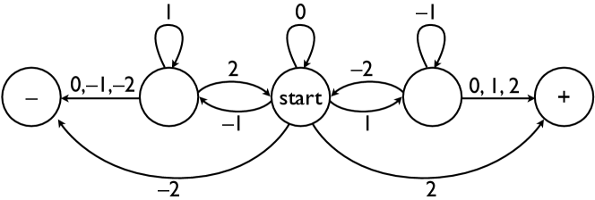
Figure 1: Finite automaton for the proof of Lemma 4.1.

We are now prepared to prove our desired upper bounds for halfspaces.

Theorem 4.2.

Let $f\colon\{-1,+1\}^{nk}\to\{-1,+1\}$ be the function given by

$$f(x)=\operatorname{sgn}\left(1+\sum_{i=1}^{n}\sum_{j=1}^{k}2^{i}x_{ij}\right).$$ (4.1)

Then

$$R^{+}(f,64k\lceil\log k\rceil+1)=0.$$ (4.2)

In addition, for all integers $d\geqslant 1,$

$$R^{+}(f,d)\leqslant 1-(k2^{n+1})^{-1/d}.$$ (4.3)

In particular, Theorem 4.2 settles all upper bounds on $\operatorname{rdeg}_{\epsilon}(f)$ in Theorem 1.6.

Proof of Theorem 4.2.

Theorem 2.4 immediately implies (4.3) in view of the representation (4.1). It remains to prove (4.2). In the degenerate case $k=1,$ we have $f\equiv x_{n1}$ and thus (4.2) holds. In what follows, we assume that $k\geqslant 2$ and put $\Delta=\lceil\log k\rceil.$ We adopt the convention that $x_{ij}\equiv 0$ for $i>n.$ For $\ell=0,1,2,\dots,$ define

$$S_{\ell}=\sum_{i=1}^{\Delta}\sum_{j=1}^{k}2^{i-1}x_{\ell\Delta+i,j}.$$

Then

$$\sum_{i=1}^{n}\sum_{j=1}^{k}2^{i-1}x_{ij}=\left(S_{0}+2^{2\Delta}S_{2}+2^{4\Delta}S_{4}+2^{6\Delta}S_{6}+\cdots\right)\\ +\left(2^{\Delta}S_{1}+2^{3\Delta}S_{3}+2^{5\Delta}S_{5}+2^{7\Delta}S_{7}+\cdots\right).$$ (4.4)

Now, each $S_{\ell}$ is an integer in $[-2^{2\Delta}+1,2^{2\Delta}-1]$ and therefore admits a representation as

$$S_{\ell}=z_{\ell,1}+2z_{\ell,2}+2^{2}z_{\ell,3}+\cdots+2^{2\Delta-1}z_{\ell,2\Delta},$$

where $z_{\ell,1},\dots,z_{\ell,2\Delta}\in\{-1,0,+1\}.$ Furthermore, each $S_{\ell}$ only depends on $k\Delta$ of the original variables $x_{ij},$ whence $z_{\ell,1},\dots,z_{\ell,2\Delta}$ can all be viewed as polynomials of degree at most $k\Delta$ in the original variables. Rewriting (4.4),

$$\sum_{i=1}^{n}\sum_{j=1}^{k}2^{i-1}x_{ij} =\left(\sum_{i\geqslant 1}2^{i-1}z_{\ell(i),j(i)}\right)+\left(\sum_{i\geqslant\Delta+1}2^{i-1}z_{\ell^{\prime}(i),j^{\prime}(i)}\right)$$

for appropriate indexing functions $\ell(i),\ell^{\prime}(i),j(i),j^{\prime}(i).$ Thus,

$$f(x)\equiv\operatorname{sgn}\left(1+\sum_{i=1}^{\Delta}2^{i}\underbrace{z_{\ell(i),j(i)}}+\sum_{i\geqslant\Delta+1}2^{i}\underbrace{\left(z_{\ell(i),j(i)}+z_{\ell^{\prime}(i),j^{\prime}(i)}\right)}\right).$$

Since the underbraced expressions range in $\{0,\pm 1,\pm 2\}$ and are polynomials of degree at most $k\Delta$ in the original variables, Lemma 4.1 implies (4.2). ∎

4.2 Preparatory work

This section sets the stage for our rational approximation lower bounds with some preparatory results about halfspaces. It will be convenient to establish some additional notation, for use in this section only. Here, we typeset real vectors in boldface ($\mathbf{x}_{1},\mathbf{x}_{2},\mathbf{z},\mathbf{v}$) to better distinguish them from scalars. The $i$th component of a vector $\mathbf{x}\in\mathbb{R}^{n}$ is denoted by $(\mathbf{x})_{i},$ while the symbol $\mathbf{x}_{i}$ is reserved for another vector from some enumeration. In keeping with this convention, we let $\mathbf{e}_{i}$ denote the vector with $1$ in the $i$th component and zeroes everywhere else. For $\mathbf{x},\mathbf{y}\in\mathbb{R}^{n},$ the vector $\mathbf{x}\mathbf{y}\in\mathbb{R}^{n}$ is given by $(\mathbf{x}\mathbf{y})_{i}\equiv(\mathbf{x})_{i}(\mathbf{y})_{i}.$ More generally, for a polynomial $p$ on $\mathbb{R}^{k}$ and vectors $\mathbf{x}_{1},\dots,\mathbf{x}_{k}\in\mathbb{R}^{n},$ we define $p(\mathbf{x}_{1},\dots,\mathbf{x}_{k})\in\mathbb{R}^{n}$ by $(p(\mathbf{x}_{1},\dots,\mathbf{x}_{k}))_{i}=p((\mathbf{x}_{1})_{i},\dots,(\mathbf{x}_{k})_{i}).$ The expectation of a random variable $\mathbf{x}\in\mathbb{R}^{n}$ is defined componentwise, i.e., the vector $\operatorname*{\mathbf{E}}[\mathbf{x}]\in\mathbb{R}^{n}$ is given by $(\operatorname*{\mathbf{E}}[\mathbf{x}])_{i}\equiv\operatorname*{\mathbf{E}}[(\mathbf{x})_{i}].$

For convenience, we adopt the notational shorthand $\alpha^{0}=1$ for all $\alpha\in\mathbb{R}.$ In particular, if $\mathbf{x}\in\mathbb{R}^{n}$ is a given vector, then $\mathbf{x}^{0}=(1,1,\dots,1)\in\mathbb{R}^{n}.$ A scalar $\alpha\in\mathbb{R},$ when interpreted as a vector, stands for $(\alpha,\alpha,\dots,\alpha).$ This shorthand allows one to speak of $\operatorname{span}\{1,\mathbf{z},\mathbf{z}^{2},\dots,\mathbf{z}^{k}\},$ for example, where $\mathbf{z}\in\mathbb{R}^{n}$ is a given vector.

Theorem 4.3.

Let $N$ and $m$ be positive integers. Then reals $\alpha_{0},\alpha_{1},\dots,\alpha_{4m}$ exist with the following property: for each $\mathbf{b}\in\{0,1\}^{N},$ there is a probability distribution $\mu_{\mathbf{b}}$ on $\{0,\pm 1,\dots,\pm m\}^{N}$ such that

$$\operatorname*{\mathbf{E}}_{\mathbf{v}\sim\mu_{\mathbf{b}}}[(2\mathbf{v}+\mathbf{b})^{d}]=(\alpha_{d},\alpha_{d},\dots,\alpha_{d}),\qquad d=0,1,2,\dots,4m.$$

Proof.

Let $\lambda_{0}$ and $\lambda_{1}$ be the distributions on $\{0,\pm 1,\dots,\pm m\}$ given by

$$\lambda_{0}(t)=16^{-m}{4m+1\choose 2m+2t},\qquad\lambda_{1}(t)=16^{-m}{4m+1\choose 2m+2t+1}.$$

Then for $d=0,1,\dots,4m,$ one has

$$\operatorname*{\mathbf{E}}_{t\sim\lambda_{0}}[(2t)^{d}]-\operatorname*{\mathbf{E}}_{t\sim\lambda_{1}}[(2t+1)^{d}]\\ =16^{-m}\sum_{t=0}^{4m+1}(-1)^{t}{4m+1\choose t}(t-2m)^{d}=0,\qquad$$ (4.5)

where (4.5) holds by Fact 2.1. Now, let $\mu_{\mathbf{b}}=\lambda_{(\mathbf{b})_{1}}\times\lambda_{(\mathbf{b})_{2}}\times\cdots\times\lambda_{(\mathbf{b})_{N}}.$ Then in view of (4.5), the theorem holds by letting $\alpha_{d}=\operatorname*{\mathbf{E}}_{\lambda_{0}}[(2t)^{d}]$ for $d=0,1,2,\dots,4m.$ ∎

Using the previous theorem, we will now establish another auxiliary result pertaining to halfspaces.

Theorem 4.4.

Put $\mathbf{z}=(-2^{n},-2^{n-1},\dots,-2^{0},2^{0},\dots,2^{n-1},2^{n})\in\mathbb{R}^{2n+2}.$ There are random variables $\mathbf{x}_{1},\mathbf{x}_{2},\dots,\mathbf{x}_{n+1}\in\{0,\pm 1,\pm 2,\dots,\pm(3n+1)\}^{2n+2}$ such that:

$$\sum_{i=1}^{n+1}2^{i-1}\mathbf{x}_{i}\equiv\mathbf{z}$$ (4.6)

and

$$\operatorname*{\mathbf{E}}\left[\prod_{i=1}^{n}\mathbf{x}_{i}^{d_{i}}\right]\in\operatorname{span}\{(1,1,\dots,1)\}$$ (4.7)

for $d_{1},\dots,d_{n}\in\{0,1,\dots,4n\}.$

Proof.

Let

$$\mathbf{x}_{i}=2\mathbf{y}_{i}-\mathbf{y}_{i-1}+\mathbf{e}_{n+1+i}-\mathbf{e}_{n+2-i},\qquad i=1,2,\dots,n+1,$$

where $\mathbf{y}_{0},\mathbf{y}_{1},\dots,\mathbf{y}_{n+1}$ are suitable random variables with $\mathbf{y}_{0}\equiv\mathbf{y}_{n+1}\equiv 0.$ Then property (4.6) is immediate. We will construct $\mathbf{y}_{0},\mathbf{y}_{1},\dots,\mathbf{y}_{n+1}$ such that the remaining property (4.7) holds as well.

Let $N=2n+2$ and $m=n$ in Theorem 4.3. Then reals $\alpha_{0},\alpha_{1},\dots,\alpha_{4n}$ exist with the property that for each $\mathbf{b}\in\{0,1\}^{2n+2},$ a probability distribution $\mu_{\mathbf{b}}$ can be found on $\{0,\pm 1,\dots,\pm n\}^{2n+2}$ such that

$$\operatorname*{\mathbf{E}}_{\mathbf{v}\sim\mu_{\mathbf{b}}}[(2\mathbf{v}+\mathbf{b})^{d}]=\alpha_{d}(1,1,\dots,1),\qquad d=0,1,\dots,4n.$$ (4.8)

Now, we will specify the distribution of $\mathbf{y}_{0},\mathbf{y}_{1},\dots,\mathbf{y}_{n}$ by giving an algorithm for generating $\mathbf{y}_{i}$ from $\mathbf{y}_{i-1}.$ First, recall that $\mathbf{y}_{0}\equiv\mathbf{y}_{n+1}\equiv 0.$ The algorithm for generating $\mathbf{y}_{i}$ given $\mathbf{y}_{i-1}$ $(i=1,2,\dots,n)$ is as follows.

• Let $\mathbf{u}$ be the unique integer vector such that $2\mathbf{u}-\mathbf{y}_{i-1}+\mathbf{e}_{n+1+i}-\mathbf{e}_{n+2-i}\in\{0,1\}^{2n+2}.$

• Draw a random vector $\mathbf{v}\sim\mu_{\mathbf{b}},$ where $\mathbf{b}=2\mathbf{u}-\mathbf{y}_{i-1}+\mathbf{e}_{n+1+i}-\mathbf{e}_{n+2-i}.$

• Set $\mathbf{y}_{i}=\mathbf{v}+\mathbf{u}.$

One easily verifies that $\mathbf{y}_{0},\mathbf{y}_{1},\dots,\mathbf{y}_{n+1}\in\{0,\pm 1,\dots,\pm 3n\}^{2n+2}.$

Let $R$ denote the resulting joint distribution of $(\mathbf{y}_{0},\mathbf{y}_{1},\dots,\mathbf{y}_{n+1}).$ Let $i\leqslant n.$ Then conditioned on any fixed value of $(\mathbf{y}_{0},\mathbf{y}_{1},\dots,\mathbf{y}_{i-1})$ in the support of $R,$ the random variable $\mathbf{x}_{i}$ is by definition independent of $\mathbf{x}_{1},\dots,\mathbf{x}_{i-1}$ and is distributed identically to $2\mathbf{v}+\mathbf{b},$ for some fixed vector $\mathbf{b}\in\{0,1\}^{2n+2}$ and a random variable $\mathbf{v}\sim\mu_{\mathbf{b}}.$ In view of (4.8), we conclude that

$$\operatorname*{\mathbf{E}}\left[\prod_{i=1}^{n}\mathbf{x}_{i}^{d_{i}}\right]=(1,1,\dots,1)\prod_{i=1}^{n}\alpha_{d_{i}}$$

for all $d_{1},d_{2},\dots,d_{n}\in\{0,1,\dots,4n\},$ which establishes (4.7). It remains to note that $\mathbf{x}_{1},\mathbf{x}_{2},\dots,\mathbf{x}_{n}\in\{-2n,-2n+1,\dots,-1,0,1,\dots,2n,2n+1\}^{2n+2},$ whereas $\mathbf{x}_{n+1}=-\mathbf{y}_{n}+\mathbf{e}_{2n+2}-\mathbf{e}_{1}\in\{0,\pm 1,\dots,\pm(3n+1)\}^{2n+2}.$ ∎

At last, we arrive at the main theorem of this section, which will play a crucial role in our analysis of the rational approximation of halfspaces.

Theorem 4.5.

For $i=0,1,2,\dots,n,$ define

$$A_{i} =\left\{(x_{1},\dots,x_{n+1})\in\{0,\pm 1,\dots,\pm(3n+1)\}^{n+1}\colon\quad\sum_{j=1}^{n+1}2^{j-1}x_{j}=2^{i}\right\}.$$

Let $p(x_{1},\dots,x_{n+1})$ be a real polynomial with sign $(-1)^{i}$ throughout $A_{i}$ $(i=0,1,2,\dots,n)$ and sign $(-1)^{i+1}$ throughout $-A_{i}$ $(i=0,1,2,\dots,n).$ Then

$$\deg p\geqslant 2n+1.$$

Proof.

For the sake of contradiction, suppose that $p$ has degree no greater than $2n.$ Put $\mathbf{z}=(-2^{n},-2^{n-1},\dots,-2^{0},2^{0},\dots,2^{n-1},2^{n}).$ Let $\mathbf{x}_{1},\dots,\mathbf{x}_{n+1}$ be the random variables constructed in Theorem 4.4. By (4.7) and the identity $\mathbf{x}_{n+1}\equiv 2^{-n}\mathbf{z}-\sum_{i=1}^{n}2^{i-n-1}\mathbf{x}_{i},$ we have

$$\operatorname*{\mathbf{E}}[p(\mathbf{x}_{1},\dots,\mathbf{x}_{n+1})]\in\operatorname{span}\{1,\mathbf{z},\mathbf{z}^{2},\dots,\mathbf{z}^{2n}\},$$

whence $\operatorname*{\mathbf{E}}[p(\mathbf{x}_{1},\dots,\mathbf{x}_{n+1})]=q(\mathbf{z})$ for a univariate polynomial $q\in P_{2n}.$ In view of (4.6) and the assumed sign behavior of $p,$ we have $\operatorname{sgn}q(2^{i})=(-1)^{i}$ and $\operatorname{sgn}q(-2^{i})=(-1)^{i+1},$ for $i=0,1,2,\dots,n.$ Therefore, $q$ has at least $2n+1$ roots. Since $q\in P_{2n},$ we arrive at a contradiction. It follows that the assumed polynomial $p$ does not exist. ∎

Remark 4.6.

The passage $p\mapsto q$ in the proof of Theorem 4.5 is precisely the linear degree-nonincreasing map $M\colon\mathbb{R}[x_{1},x_{2},\dots,x_{n+1}]\to\mathbb{R}[x]$ described previously in the Introduction.

4.3 Lower bounds

The purpose of this section is to prove that the canonical halfspace cannot be approximated well by a rational function of low degree. A starting point in our discussion is a criterion for inapproximability by low-degree rational functions, which is applicable not only to halfspaces but any odd Boolean functions on Euclidean space.

Theorem 4.7 (Criterion for inapproximability).

Fix a nonempty finite subset $S\subset\mathbb{R}^{m}$ with $S\cap-S=\varnothing.$ Define $f\colon S\cup-S\to\{-1,+1\}$ by

$$f(x)=\begin{cases}+1,&x\in S,\\ -1,&x\in-S.\end{cases}$$

Let $\psi$ be a real function such that

$$\psi(x)>\delta|\psi(-x)|, x\in S,$$ (4.9)

for some $\delta\in(0,1)$ and

$$\sum_{S\cup-S}\psi(x)u(x)=0$$ (4.10)

for every polynomial $u$ of degree at most $d.$ Then

$$R^{+}(f,d)\geqslant\frac{2\delta}{1+\delta}.$$

Proof.

Fix polynomials $p,q$ of degree at most $d$ such that $q$ is positive on $S\cup-S.$ Put

$$\epsilon=\max_{S\cup-S}\left|f(x)-\frac{p(x)}{q(x)}\right|.$$

We assume that $\epsilon<1$ since otherwise there is nothing to show. For $x\in S,$

$$(1-\epsilon)q(x)\leqslant p(x)\leqslant(1+\epsilon)q(x)$$ (4.11)

and

$$(1-\epsilon)q(-x)\leqslant-p(-x)\leqslant(1+\epsilon)q(-x).$$ (4.12)

Consider the polynomial $u(x)=q(x)+q(-x)+p(x)-p(-x).$ Equations (4.11) and (4.12) show that for $x\in S,$ one has $u(x)\geqslant(2-\epsilon)\{q(x)+q(-x)\}$ and $|u(-x)|\leqslant\epsilon\{q(x)+q(-x)\},$ whence

$$u (x)\geqslant\left(\frac{2}{\epsilon}-1\right)|u(-x)|, x\in S.$$ (4.13)

We also note that

$$u (x)>0, x\in S.$$ (4.14)

Since $u$ has degree at most $d,$ we have by (4.10) that

$$\sum_{x\in S}\{\psi(x)u(x)+\psi(-x)u(-x)\}=\sum_{S\cup-S}\psi(x)u(x)=0,$$

whence

$$\psi(x)u(x)\leqslant|\psi(-x)u(-x)|$$

for some $x\in S.$ At the same time, it follows from (4.9), (4.13), and (4.14) that

$$\psi(x)u(x)>\delta\left(\frac{2}{\epsilon}-1\right)\lvert\psi(-x)u(-x)\rvert, x\in S.$$

We immediately obtain $\delta(\{2/\epsilon\}-1)<1,$ as was to be shown. ∎

Remark 4.8.

The method of Theorem 4.7 amounts to reformulating (4.13) and (4.14) as a linear program and exhibiting a solution to its dual. The presentation above does not explicitly use the language of linear programs or appeal to duality, however, because our goal is solely to prove the correctness of our method and not its completeness.

Using the criterion of Theorem 4.7 and our preparatory work in Section 4.2, we now establish a key lower bound for the rational approximation of halfspaces within constant error.

Theorem 4.9.

Let $f\colon\{0,\pm 1,\dots,\pm(3n+1)\}^{n+1}\to\{-1,+1\}$ be given by

$$f(x)=\operatorname{sgn}\left(1+\sum_{i=1}^{n+1}2^{i}x_{i}\right).$$

Then

$$R^{+}(f,n)=\Omega(1).$$

Proof.

Let $A_{0},A_{1},\dots,A_{n}$ be as defined in Theorem 4.5. Put $A=\bigcup A_{i}$ and define $g\colon A\cup-A\to\{-1,+1\}$ by

$$g(x)=\begin{cases}(-1)^{i},&x\in A_{i},\\ (-1)^{i+1},&x\in-A_{i}.\end{cases}$$

Then $\operatorname{deg_{\pm}}(f)>2n$ by Theorem 4.5. As a result, Theorem 2.2 guarantees the existence of a function $\phi\colon A\cup-A\to\mathbb{R},$ not identically zero, such that

$$\phi(x)g(x)\geqslant 0,\qquad x\in A\cup-A,$$ (4.15)

and

$$\sum_{A\cup-A}\phi(x)u(x)=0$$ (4.16)

for every polynomial $u$ of degree at most $2n.$ Put

$$p(x)=\prod_{j=0}^{n-1}\left(-2^{j}\sqrt{2}+\sum_{i=1}^{n+1}2^{i-1}x_{i}\right)$$

and

$$\psi(x)=(-1)^{n}\{\phi(x)-\phi(-x)\}p(x).$$

Define $S=A\setminus\psi^{-1}(0).$ Then $S\neq\varnothing$ by (4.15) and the fact that $\phi$ is not identically zero on $A\cup-A.$ For $x\in S,$ we have $\psi(-x)\neq 0$ and

$$\frac{\lvert\psi(x)\rvert}{\lvert\psi(-x)\rvert}=\frac{\lvert p(x)\rvert}{\lvert p(-x)\rvert}>\left(\prod_{i=1}^{\infty}\frac{2^{i/2}-1}{2^{i/2}+1}\right)^{2}>\exp(-9\sqrt{2}),$$

where the final step uses the bound $(a-1)/(a+1)>\exp(-2.5/a),$ valid for $a\geqslant\sqrt{2}.$ It follows from (4.15) and the definition of $p$ that $\psi$ is positive on $S.$ Hence,

$$\psi(x)>\exp(-9\sqrt{2})\;\lvert\psi(-x)\rvert,\qquad x\in S.$$ (4.17)

For any polynomial $u$ of degree no greater than $n,$ we infer from (4.16) that

$$\sum_{S\cup-S}\psi(x)u(x)=(-1)^{n}\sum_{A\cup-A}\{\phi(x)-\phi(-x)\}u(x)p(x)=0.$$ (4.18)

Since $f$ is positive on $S$ and negative on $-S,$ the proof is now complete in view of (4.17), (4.18), and Theorem 4.7. ∎

We have reached the main result of this section, which extends Theorem 4.9 to any subconstant approximation error and to halfspaces on the hypercube.

Theorem 4.10.

Let $F\colon\{-1,+1\}^{m^{2}}\to\{-1,+1\}$ be given by

$$F(x)=\operatorname{sgn}\left(1+\sum_{i=1}^{m}\sum_{j=1}^{m}2^{i}x_{ij}\right).$$

Then for $d<m/14,$

$$R(F,d)\geqslant 1-2^{-\Theta(m/d)}.$$ (4.19)

Observe that Theorem 4.10 settles the lower bounds in Theorem 1.6 from the Introduction.

Proof of Theorem 4.10..

We may assume that $m\geqslant 14,$ the claim being trivial otherwise. Consider the function $G\colon\{-1,+1\}^{(n+1)(6n+2)}\to\{-1,+1\}$ given by

$$G(x)=\operatorname{sgn}\left(1+\sum_{i=1}^{n+1}\;\sum_{j=1}^{6n+2}2^{i}x_{ij}\right),$$

where $n=\lfloor(m-2)/6\rfloor.$ For every $\epsilon>R^{+}(G,n),$ Proposition 2.7 provides a rational function $A$ on $\mathbb{R}^{n+1}$ of degree at most $n$ such that, on the domain of $G,$

$$\left\lvert G(x)-A\left(\dots,\sum_{j=1}^{6n+2}x_{ij},\dots\right)\right\rvert<\epsilon$$

and the denominator of $A$ is positive. Letting $f$ be the function in Theorem 4.9, it follows that $|f(x_{1},\dots,x_{n+1})-A(2x_{1},\dots,2x_{n+1})|<\epsilon$ on the domain of $f,$ whence

$$R^{+}(G,n)=\Omega(1).$$ (4.20)

We now claim that either $G(x)$ or $-G(-x)$ is a subfunction of $F.$ For example, consider the following substitution for the variables $x_{ij}$ for which $i>n+1$ or $j>6n+2$:

$$x_{mj}\leftarrow(-1)^{j}, (1\leqslant j\leqslant m),$$

$$x_{ij}\leftarrow(-1)^{j+1}, (n+1<i<m,\quad 1\leqslant j\leqslant m),$$

$$x_{ij}\leftarrow(-1)^{j+1}, (1\leqslant i\leqslant n+1,\quad\,j>6n+2).$$

After this substitution, $F$ is a function of the remaining variables $x_{ij}$ and is equivalent to $G(x)$ if $m$ is even, and to $-G(-x)$ if $m$ is odd. In either case, (4.20) implies that

$$R^{+}(F,n)=\Omega(1).$$ (4.21)

Theorem 2.5 shows that

$$R(F,n/2)\leqslant 1-\left(\frac{1-R(F,d)}{2}\right)^{1/\lfloor n/(2d)\rfloor}$$

for $d=1,2,\dots,\lfloor n/2\rfloor,$ which yields (4.19) in light of (2.2) and (4.21). ∎

5 Rational approximation of the majority function

The goal of this section is to determine $R^{+}(\text{\rm MAJ}_{n},d)$ for each integer $d,$ i.e., to determine the least error to which a degree-$d$ multivariate rational function can approximate the majority function. As is frequently the case with symmetric Boolean functions such as majority, the multivariate problem of analyzing $R^{+}(\text{\rm MAJ}_{n},d)$ is equivalent to a univariate question. Specifically, given an integer $d$ and a finite set $S\subset\mathbb{R},$ we define

$$R^{+}(d,S)\,=\,\inf_{p,q}\,\max_{t\in S}\left\lvert\operatorname{sgn}t-\frac{p(t)}{q(t)}\right\rvert,$$

where the infimum ranges over $p,q\in P_{d}$ such that $q$ is positive on $S.$ In other words, we study how well a rational function of a given degree can approximate the sign function over a finite support. We give a detailed answer to this question in the following theorem:

Theorem 5.1 (Rational approximation of majority).

Let $n,d$ be positive integers. Abbreviate $R=R^{+}(d,\{\pm 1,\pm 2,\dots,\pm n\}).$ For $1\leqslant d\leqslant\log n,$

$$\exp\left\{-\Theta\left(\frac{1}{n^{1/(2d)}}\right)\right\}\leqslant R<\exp\left\{-\frac{1}{n^{1/d}}\right\}.$$

For $\log n<d<n,$

$$R=\exp\left\{-\Theta\left(\frac{d}{\log(2n/d)}\right)\right\}.$$

For $d\geqslant n,$

$$R=0.$$

Moreover, the rational approximant is constructed explicitly in each case.

Theorem 5.1 is the main result of this section. We establish it in the next two subsections, giving separate treatment to the cases $d\leqslant\log n$ and $d>\log n$ (see Theorems 5.3 and 5.8, respectively). In the concluding subsection, we give the promised proof that $R^{+}(d,\{\pm 1,\dots,\pm n\})$ and $R^{+}(\text{\rm MAJ}_{n},d)$ are essentially equivalent.

5.1 Low-degree approximation

We start by specializing the criterion of Theorem 4.7 to the problem of approximating the sign function on the set $\{\pm 1,\pm 2,\dots,\pm n\}.$

Theorem 5.2.

Let $d$ be an integer, $0\leqslant d\leqslant 2n-1.$ Fix a nonempty subset $S\subseteq\{1,2,\dots,n\}.$ Suppose that there exists a real $\delta\in(0,1)$ and a polynomial $r\in P_{\,2n-d-1}$ that vanishes on $\{-n,\dots,n\}\setminus(S\cup-S)$ and obeys

$$(-1)^{t}r(t)>\delta\lvert r(-t)\rvert,\qquad t\in S.$$ (5.1)

Then

$$R^{+}(d,S\cup-S)\geqslant\frac{2\delta}{1+\delta}.$$ (5.2)

Proof.

Define $f\colon S\cup-S\to\{-1,+1\}$ by $f(t)=\operatorname{sgn}t.$ Define $\psi\colon S\cup-S\to\mathbb{R}$ by $\psi(t)=(-1)^{t}{2n\choose n+t}r(t).$ Then (5.1) takes on the form

$$\psi(t)>\delta\lvert\psi(-t)\rvert,\qquad t\in S.$$ (5.3)

For every polynomial $u$ of degree at most $d,$ we have

$$\sum_{S\cup-S}\psi(t)u(t)=\sum_{t=-n}^{n}(-1)^{t}{2n\choose n+t}r(t)u(t)=0$$ (5.4)

by Fact 2.1. Now (5.2) is immediate from (5.3), (5.4), and Theorem 4.7. ∎

Using Theorem 5.2, we will now determine the optimal error in the approximation of the majority function by rational functions of degree up to $\log n.$ The case of higher degrees will be settled in the next subsection.

Theorem 5.3 (Low-degree rational approximation of majority).

Let $d$ be an integer, $1\leqslant d\leqslant\log n.$ Then

$$\exp\left\{-\Theta\left(\frac{1}{n^{1/(2d)}}\right)\right\}\leqslant R^{+}(d,\{\pm 1,\pm 2,\dots,\pm n\})<\exp\left\{-\frac{1}{n^{1/d}}\right\}.$$

Proof.

The upper bound is immediate from Newman’s Theorem 2.4. For the lower bound, put $\Delta=\lfloor n^{1/d}\rfloor\geqslant 2$ and $S=\{1,\Delta,\Delta^{2},\dots,\Delta^{d}\}.$ Define $r\in P_{\,2n-d-1}$ by

$$r(t)=(-1)^{n}\prod_{i=0}^{d-1}(t-\Delta^{i}\sqrt{\Delta})\prod_{i\in\{-n,\dots,n\}\setminus(S\cup-S)}(t-i).$$

For $j=0,1,2,\dots,d,$

$$\frac{|r(\Delta^{j})|}{|r(-\Delta^{j})|} =\prod_{i=0}^{j-1}\frac{\Delta^{j}-\Delta^{i}\sqrt{\Delta}}{\Delta^{j}+\Delta^{i}\sqrt{\Delta}}\;\prod_{i=j}^{d-1}\frac{\Delta^{i}\sqrt{\Delta}-\Delta^{j}}{\Delta^{i}\sqrt{\Delta}+\Delta^{j}}>\left(\prod_{i=1}^{\infty}\frac{\Delta^{i/2}-1}{\Delta^{i/2}+1}\right)^{2}$$

$$>\exp\left\{-5\sum_{i=1}^{\infty}\frac{1}{\Delta^{i/2}}\right\}>\exp\left\{-\frac{18}{\sqrt{\Delta}}\right\},$$

where we used the bound $(a-1)/(a+1)>\exp(-2.5/a),$ valid for $a\geqslant\sqrt{2}.$ Since $\operatorname{sgn}r(t)=(-1)^{t}$ for $t\in S,$ we conclude that

$$(-1)^{t}r(t)>\exp\left\{-\frac{18}{\sqrt{\Delta}}\right\}\lvert r(-t)\rvert,\qquad t\in S.$$

Since in addition $r$ vanishes on $\{-n,\dots,n\}\setminus(S\cup-S),$ we infer from Theorem 5.2 that $R^{+}(d,S\cup-S)\geqslant\exp\{-18/\sqrt{\Delta}\}.$ ∎

5.2 High-degree approximation

In the previous subsection, we determined the least error in approximating the majority function by rational functions of degree up to $\log n.$ Our goal here is to solve the case of higher degrees.

We start with some preparatory work. First, we need to accurately estimate products of the form $\prod_{i}(\Delta^{i}+1)/(\Delta^{i}-1)$ for all $\Delta>1.$ A suitable lower bound was already given by Newman [31, Lem. 1]:

Lemma 5.4 (Newman).

For all $\Delta>1,$

$$\prod_{i=1}^{n}\frac{\Delta^{i}+1}{\Delta^{i}-1}>\exp\left\{\frac{2(\Delta^{n}-1)}{\Delta^{n}(\Delta-1)}\right\}.$$

Proof.

Immediate from the bound $(a+1)/(a-1)>\exp(2/a),$ which is valid for $a>1.$ ∎

We will need a corresponding upper bound:

Lemma 5.5.

For all $\Delta>1,$

$$\prod_{i=1}^{\infty}\frac{\Delta^{i}+1}{\Delta^{i}-1}<\exp\left\{\frac{4}{\Delta-1}\right\}.$$

Proof.

Let $k\geqslant 0$ be an integer. By the binomial theorem, $\Delta^{i}\geqslant(\Delta-1)i+1$ for integers $i\geqslant 0.$ As a result,

$$\prod_{i=1}^{k}\frac{\Delta^{i}+1}{\Delta^{i}-1}\leqslant\prod_{i=1}^{k}\frac{1}{i}\left(i+\frac{2}{\Delta-1}\right)\leqslant{k+\left\lceil\frac{2}{\Delta-1}\right\rceil\choose k}.$$

Also,

$$\prod_{i=k+1}^{\infty}\frac{\Delta^{i}+1}{\Delta^{i}-1}<\prod_{i=0}^{\infty}\left(1+\frac{2}{(\Delta^{k+1}-1)\Delta^{i}}\right)<\exp\left\{\frac{2\Delta}{(\Delta^{k+1}-1)(\Delta-1)}\right\}.$$

Setting $k=k(\Delta)=\left\lfloor\frac{2}{\Delta-1}\right\rfloor,$ we conclude that

$$\prod_{i=1}^{\infty}\frac{\Delta^{i}+1}{\Delta^{i}-1}<\exp\left\{\frac{C}{\Delta-1}\right\},$$

where

$$C=\sup_{\Delta>1}\left\{(\Delta-1)\ln{k(\Delta)+\left\lceil\frac{2}{\Delta-1}\right\rceil\choose k(\Delta)}+\frac{2\Delta}{\Delta^{k(\Delta)+1}-1}\right\}<4.$$ ∎

We will also need the following binomial estimate.

Lemma 5.6.

Put $p(t)=\prod_{i=1}^{n}\left(t-i-\frac{1}{2}\right).$ Then

$$\max_{t=1,2,\dots,n+1}\left\lvert\frac{p(-t)}{p(t)}\right\rvert\leqslant\Theta(16^{n}).$$

Proof.

For $t=1,2,\dots,n+1,$ we have

$$|p(t)|=\frac{(2t-2)!(2n-2t+2)!}{4^{n}(t-1)!(n-t+1)!},\quad|p(-t)|=\frac{t!(2n+2t+1)!}{4^{n}(2t+1)!(n+t)!}.$$

As a result,

$$\left\lvert\frac{p(-t)}{p(t)}\right\rvert =\frac{t}{2t+1}\cdot\frac{\displaystyle{2n+2t+1\choose 2t}{2n+1\choose n+t}}{\displaystyle{2t-2\choose t-1}{2n-2t+2\choose n-t+1}}\leqslant\frac{\displaystyle\Theta\left(\frac{2^{4n}}{\sqrt{n}}\right)\Theta\left(\frac{2^{2n}}{\sqrt{n}}\right)}{\displaystyle\Theta\left(\frac{2^{2n}}{n}\right)},$$

which gives the sought bound. ∎

Our construction requires one additional ingredient.

Lemma 5.7.

Let $n,d$ be integers, $1\leqslant d\leqslant n/55.$ Consider the polynomial $p(t)=\prod_{i=1}^{d-1}(t-d\Delta^{i}\sqrt{\Delta}),$ where $\Delta=(n/d)^{1/d}.$ Then

$$\min_{j=1,\dots,d}\left|\frac{p(\lfloor d\Delta^{j}\rfloor)}{p(-\lfloor d\Delta^{j}\rfloor)}\right|>\exp\left\{-\frac{4\ln 3d}{\ln(n/d)}-\frac{8}{\sqrt{\Delta}-1}\right\}.$$

Proof.

Fix $j=1,2,\dots,d.$ Then for each $i=1,2,\dots,j-1,$

$$d\Delta^{j}-d\Delta^{i}\sqrt{\Delta}\geqslant d\left(\Delta^{j-i-\frac{1}{2}}-1\right)\geqslant\frac{1}{2}\,(j-i)\ln\frac{n}{d},$$

and thus

$$\prod_{i=1}^{j-1}\left(1-\frac{1}{d\Delta^{j}-d\Delta^{i}\sqrt{\Delta}}\right) \geqslant\exp\left\{-\frac{4}{\ln(n/d)}\sum_{i=1}^{j-1}\frac{1}{j-i}\right\}$$

$$\geqslant\exp\left\{-\frac{4\ln 3d}{\ln(n/d)}\right\}.$$ (5.5)

For brevity, let $\xi$ stand for the final expression in (5.5). Since $1\leqslant d\leqslant n/55,$ we have $\lfloor d\Delta^{j}\rfloor-d\Delta^{j-1}\sqrt{\Delta}>1.$ As a result,

$$\left|\frac{p(\lfloor d\Delta^{j}\rfloor)}{p(-\lfloor d\Delta^{j}\rfloor)}\right| \geqslant\prod_{i=1}^{j-1}\frac{d\Delta^{j}-1-d\Delta^{i}\sqrt{\Delta}}{d\Delta^{j}+d\Delta^{i}\sqrt{\Delta}}\;\;\prod_{i=j}^{d-1}\frac{d\Delta^{i}\sqrt{\Delta}-d\Delta^{j}}{d\Delta^{i}\sqrt{\Delta}+d\Delta^{j}}$$

$$\geqslant\xi\prod_{i=1}^{j-1}\frac{d\Delta^{j}-d\Delta^{i}\sqrt{\Delta}}{d\Delta^{j}+d\Delta^{i}\sqrt{\Delta}}\;\;\prod_{i=j}^{d-1}\frac{d\Delta^{i}\sqrt{\Delta}-d\Delta^{j}}{d\Delta^{i}\sqrt{\Delta}+d\Delta^{j}}$$ by (5.5)

$$>\xi\left(\prod_{i=1}^{\infty}\frac{\Delta^{i/2}-1}{\Delta^{i/2}+1}\right)^{2}$$

$$\geqslant\xi\exp\left\{-\frac{8}{\sqrt{\Delta}-1}\right\},$$

where the last inequality holds by Lemma 5.5. ∎

We have reached the main result of this subsection.

Theorem 5.8 (High-degree rational approximation of majority).

Let $d$ be an integer, $\log n<d\leqslant n-1.$ Then

$$R^{+}(d,\{\pm 1,\pm 2,\dots,\pm n\})=\exp\left\{-\Theta\left(\frac{d}{\log(2n/d)}\right)\right\}.$$

Also,

$$R^{+}(n,\{\pm 1,\pm 2,\dots,\pm n\})=0.$$

Proof.

The final statement in the theorem follows at once by considering the rational function $\{p(t)-p(-t)\}/\{p(t)+p(-t)\},$ where $p(t)=\prod_{i=1}^{n}(t+i).$

Now assume that $\log n<d<n/55.$ Let

$$k=\left\lceil\frac{d}{\log(n/d)}\right\rceil,\qquad\Delta=\left(\frac{n}{d}\right)^{1/d}.$$

Define sets

$$S_{1} =\{1,2,\dots,k\},$$

$$S_{2} =\rule{0.0pt}{11.38109pt}\{\lfloor d\Delta^{i}\rfloor\,:\,i=1,2,\dots,d\},$$

$$S_{\phantom{1}} =\rule{0.0pt}{11.38109pt}S_{1}\cup S_{2}.$$

Consider the polynomial

$$r(t)=(-1)^{n}r_{1}(t)r_{2}(t)\prod_{i\in\{-n,\dots,n\}\setminus(S\cup-S)}(t-i),$$

where

$$r_{1}(t)=\prod_{i=1}^{k}\left(t-i-\frac{1}{2}\right),\qquad r_{2}(t)=\prod_{i=1}^{d-1}(t-d\Delta^{i}\sqrt{\Delta}).$$

We have:

$$\min_{t\in S}\left|\frac{r(t)}{r(-t)}\right| \geqslant\min_{i=1,\dots,k+1}\left|\frac{r_{1}(i)}{r_{1}(-i)}\right|\cdot\min_{i=1,\dots,d}\left|\frac{r_{2}(\lfloor d\Delta^{i}\rfloor)}{r_{2}(-\lfloor d\Delta^{i}\rfloor)}\right|$$

$$>\exp\left\{-\frac{Cd}{\log(n/d)}\right\}$$

by Lemmas 5.6 and 5.7, where $C>0$ is an absolute constant. Since $\operatorname{sgn}p(t)=(-1)^{t}$ for $t\in S,$ we can restate this result as follows:

$$(-1)^{t}r(t)>\exp\left\{-\frac{Cd}{\log(n/d)}\right\}|r(-t)|,\qquad t\in S.$$

Since $r$ vanishes on $\{-n,\dots,n\}\setminus(S\cup-S)$ and has degree $\leqslant 2n-1-d,$ we infer from Theorem 5.2 that $R^{+}(d,S\cup-S)\geqslant\exp\left\{-Cd/\log(n/d)\right\}.$ This proves the lower bound for the case $\log n<d<n/55.$

To handle the case $n/55\leqslant d\leqslant n-1,$ a different argument is needed. Let

$$r(t)=(-1)^{n}\,t\,\prod_{i=1}^{d}\left(t-i-\frac{1}{2}\right)\prod_{i=d+2}^{n}(t^{2}-i^{2}).$$

By Lemma 5.6, there is an absolute constant $C>1$ such that

$$\left\lvert\frac{r(t)}{r(-t)}\right\rvert>C^{-d},\qquad t=1,2,\dots,d+1.$$

Since $\operatorname{sgn}r(t)=(-1)^{t}$ for $t=1,2,\dots,d+1,$ we conclude that

$$(-1)^{t}r(t)>C^{-d}|r(-t)|,\qquad t=1,2,\dots,d+1.$$

Since the polynomial $r$ vanishes on $\{-n,\dots,n\}\setminus\{\pm 1,\pm 2,\dots,\pm(d+1)\}$ and has degree $2n-1-d,$ we infer from Theorem 5.2 that

$$R^{+}(d,\{\pm 1,\pm 2,\dots,\pm(d+1)\})\geqslant C^{-d}.$$

This settles the lower bound for the case $n/55\leqslant d\leqslant n-1.$

It remains to prove the upper bound for the case $\log n<d\leqslant n-1.$ Here we always have $d\geqslant 2.$ Letting $k=\lfloor d/2\rfloor$ and $\Delta=(n/k)^{1/k},$ define $p\in P_{\,2k}$ by

$$p(t)=\prod_{i=1}^{k}(t+i)\prod_{i=1}^{k}(t+k\Delta^{i}).$$

Fix any point $t\in\{1,2,\dots,n\}$ with $p(-t)\neq 0.$ Letting $i^{*}$ be the integer with $k\Delta^{i^{*}}<t<k\Delta^{i^{*}+1},$ we have:

$$\frac{p(t)}{|p(-t)|} >\prod_{i=0}^{i^{*}}\frac{k\Delta^{i^{*}+1}+k\Delta^{i}}{k\Delta^{i^{*}+1}-k\Delta^{i}}\prod_{i=i^{*}+1}^{k}\frac{k\Delta^{i}+k\Delta^{i^{*}}}{k\Delta^{i}-k\Delta^{i^{*}}}\geqslant\prod_{i=1}^{k}\frac{\Delta^{i}+1}{\Delta^{i}-1}$$

$$>\exp\left\{\frac{2(\Delta^{k}-1)}{\Delta^{k}(\Delta-1)}\right\},$$

where the last inequality holds by Lemma 5.4. Substituting $\Delta=(n/k)^{1/k}$ and recalling that $k\geqslant\Theta(\log n),$ we obtain $p(t)>A|p(-t)|$ for $t=1,2,\dots,n,$ where

$$A=\exp\left\{\Theta\left(\frac{k}{\log(n/k)}\right)\right\}.$$

As a result, $R^{+}(2k,\{\pm 1,\pm 2,\dots,\pm n\})\leqslant 2A/(A^{2}+1),$ the approximant in question being

$$\frac{A^{2}-1}{A^{2}+1}\cdot\frac{p(t)-p(-t)}{p(t)+p(-t)}.$$ ∎

5.3 Equivalence of the majority and sign functions

It remains to prove the promised equivalence of the majority and sign functions, from the standpoint of approximating them by rational functions on the discrete domain. We have:

Theorem 5.9.

For every integer $d,$

$$R^{+}(\text{\rm MAJ}_{n},d) \leqslant R^{+}(d-2,\{\pm 1,\pm 2,\dots,\pm\lceil n/2\rceil\}),$$ (5.6)

$$R^{+}(\text{\rm MAJ}_{n},d) \geqslant R^{+}(d,\{\pm 1,\pm 2,\dots,\pm\lfloor n/2\rfloor\}).$$ (5.7)

Proof.

We prove (5.6) first. Fix a degree-$(d-2)$ approximant $p(t)/q(t)$ to $\operatorname{sgn}t$ on $S=\{\pm 1,\dots,\pm\lceil n/2\rceil\},$ where $q$ is positive on $S.$ For small $\delta>0,$ define

$$A_{\delta}(t)=\frac{t^{2}p(t)-\delta}{t^{2}q(t)+\delta}.$$

Then $A_{\delta}$ is a rational function of degree at most $d$ whose denominator is positive on $S\cup\{0\}.$ Finally, we have $A_{\delta}(0)=-1$ and

$$\lim_{\delta\to 0}\max_{t\in S}|\operatorname{sgn}t-A_{\delta}(t)|=\max_{t\in S}\left|\operatorname{sgn}t-\frac{p(t)}{q(t)}\right|.$$

Then $A_{\delta}(\frac{1}{2}\sum(x_{i}+1)-\lfloor n/2\rfloor)$ is the desired approximant for $\text{\rm MAJ}_{n}(x_{1},\dots,x_{n}).$

We now turn to the lower bound, (5.7). For every $\epsilon>R^{+}(\text{\rm MAJ}_{n},d),$ Proposition 2.7 gives a univariate rational function $p(t)/q(t)$ of degree at most $d$ such that for all $x\in\{-1,+1\}^{n},$ one has

$$\left\lvert\text{\rm MAJ}_{n}(x)-\frac{p(\sum x_{i})}{q(\sum x_{i})}\right\rvert<\epsilon$$

and $q(\sum x_{i})>0.$ Then

$$\max_{t=\pm 1,\pm 2,\dots,\pm\lfloor n/2\rfloor}\left|\operatorname{sgn}t-\frac{p(2t+n-2\lfloor n/2\rfloor)}{q(2t+n-2\lfloor n/2\rfloor)}\right|<\epsilon,$$

completing the proof of (5.7). ∎

Note that (2.2) and Theorems 5.3, 5.8, and 5.9 immediately imply Theorem 1.7 from the Introduction.

Remark 5.10.

The proof that we gave for the upper bound, (5.6), illustrates a useful property of univariate rational approximants $A(t)=p(t)/q(t)$ on a finite set $S.$ Specifically, given such an approximant and a point $t^{*}\notin S,$ there exists an approximant $A^{\prime}$ with $A^{\prime}(t^{*})=a$ for any prescribed value $a$ and $A^{\prime}\approx A$ everywhere on $S.$ One such construction is

$$A^{\prime}(t)=\frac{(t-t^{*})p(t)+a\delta}{(t-t^{*})q(t)+\delta}$$

for an arbitrarily small constant $\delta>0.$ Note that $A^{\prime}$ has degree only $1$ higher than the degree of the original approximant, $A.$ This phenomenon is in sharp contrast to approximation by polynomials, which do not possess this corrective ability.

6 Intersections of halfspaces

In this section, we prove our main theorems on the sign-representation of intersections of halfspaces and majority functions. In the two subsections that follow, we give results for the threshold degree as well as threshold density, another key complexity measure of a sign-representation.

6.1 Lower bounds on the threshold degree

We start by formalizing the elegant observation due to Beigel et al. [9], already described briefly in the Introduction.

Theorem 6.1 (Beigel, Reingold, and Spielman).

Let $f\colon X\to\{-1,+1\}$ and $g\colon Y\to\{-1,+1\}$ be given functions, where $X,Y\subset\mathbb{R}^{n}$ are finite sets. Let $d$ be an integer with $R^{+}(f,d)+R^{+}(g,d)<1.$ Then

$$\operatorname{deg_{\pm}}(f\wedge g)\leqslant 2d.$$

Proof.

Fix rational functions $p_{1}(x)/q_{1}(x)$ and $p_{2}(y)/q_{2}(y)$ of degree at most $d$ such that $q_{1}$ and $q_{2}$ are positive on $X$ and $Y,$ respectively, and

$$\max_{x\in X}\left|f(x)-\frac{p_{1}(x)}{q_{1}(x)}\right|+\max_{y\in Y}\left|g(y)-\frac{p_{2}(y)}{q_{2}(y)}\right|<1.$$

Then

$$f(x)\wedge g(y)\equiv\operatorname{sgn}\{1+f(x)+g(y)\}\equiv\operatorname{sgn}\left\{1+\frac{p_{1}(x)}{q_{1}(x)}+\frac{p_{2}(y)}{q_{2}(y)}\right\}.$$

Multiplying the last expression by the positive quantity $q_{1}(x)q_{2}(y),$ we obtain $f(x)\wedge g(y)\equiv\operatorname{sgn}\{q_{1}(x)q_{2}(y)+p_{1}(x)q_{2}(y)+p_{2}(y)q_{1}(x)\}.$ ∎

Recall that Theorem 3.17 gives an essentially exact converse to Theorem 6.1. We are now in a position to prove our main results on the threshold degree.

Theorem 6.2 (restatement of Theorems 1.8 and 1.10).

Consider the function $f\colon\{-1,+1\}^{n^{2}}\to\{-1,+1\}$ given by

$$f(x)=\operatorname{sgn}\left(1+\sum_{i=1}^{n}\sum_{j=1}^{n}2^{i}x_{ij}\right).$$

Let $g\colon\{-1,+1\}^{n}\to\{-1,+1\}$ be the majority function on $n$ bits. Then

$$\operatorname{deg_{\pm}}(f\wedge f) =\Omega(n),$$ (6.1)

$$\operatorname{deg_{\pm}}(\,g\,\wedge\,g\,) =\Omega(\log n).$$ (6.2)

Proof.

By Theorem 4.10, we have $R^{+}(f,\epsilon n)\geqslant 1/2$ for some constant $\epsilon>0,$ which settles (6.1) in view of Theorem 3.17.

Analogously, Theorems 5.1 and 5.9 show that $R^{+}(g,\epsilon\log n)\geqslant 1/2$ for some constant $\epsilon>0,$ which settles (6.2) in view of Theorem 3.17. ∎

Remark 6.3.

The lower bounds (6.1) and (6.2) are tight and match the constructions due to Beigel et al. [9]. These matching upper bounds can be seen as follows. By Theorem 4.2, we have $R^{+}(f,Cn)<1/2$ for some constant $C>0,$ which shows that $\operatorname{deg_{\pm}}(f\wedge f)=O(n)$ in view of Theorem 6.1. Analogously, Theorems 5.1 and 5.9 imply that $R^{+}(g,C\log n)<1/2$ for some constant $C>0,$ which shows that $\operatorname{deg_{\pm}}(g\wedge g)=O(\log n)$ in view of Theorem 6.1.

Furthermore, Theorem 6.1 generalizes immediately to conjunctions of $k=3$ and more functions. In particular, the lower bounds in (6.1) and (6.2) remain tight for intersections $f\wedge f\wedge\cdots\wedge f$ and $g\wedge g\wedge\cdots\wedge g$ featuring any constant number of functions.

We give one additional result, featuring the intersection of the canonical halfspace with a majority function.

Theorem 1.9 (restated). Let $f\colon\{-1,+1\}^{n^{2}}\to\{-1,+1\}$ be given by

$$f(x)=\operatorname{sgn}\left(1+\sum_{i=1}^{n}\sum_{j=1}^{n}2^{i}x_{ij}\right).$$

Let $g\colon\{-1,+1\}^{\lceil\sqrt{n}\rceil}\to\{-1,+1\}$ be the majority function on $\lceil\sqrt{n}\rceil$ bits. Then

$$\operatorname{deg_{\pm}}(f\wedge\,g\,) =\Theta(\sqrt{n}).$$ (6.3)

Proof.

We prove the lower bound first. Let $\epsilon>0$ be a suitably small constant. By Theorem 4.10, we have $R^{+}(f,\epsilon\sqrt{n})\geqslant 1-2^{-\sqrt{n}}.$ By Theorems 5.1 and 5.9, we have $R^{+}(g,\epsilon\sqrt{n})\geqslant 2^{-\sqrt{n}}.$ In view of Theorem 3.17, these two facts imply that $\operatorname{deg_{\pm}}(f\wedge g\,)=\Omega(\sqrt{n}).$

We now turn to the upper bound. It is clear that $R^{+}(g,\lceil\sqrt{n}\rceil)=0$ and $R^{+}(f,1)<1.$ It follows by Theorem 6.1 that $\operatorname{deg_{\pm}}(f\wedge g)=O(\sqrt{n}).$ ∎

6.2 Lower bounds on the threshold density

In addition to threshold degree, several other complexity measures are of interest when sign-representing Boolean functions by real polynomials. One such complexity measure is density, i.e., the number of distinct monomials in any polynomial that sign-represents a given function. Formally, for a given function $f\colon\{-1,+1\}^{n}\to\{-1,+1\},$ the threshold density $\operatorname{dns}(f)$ is the minimum $k$ such that

$$f(x)\equiv\operatorname{sgn}\left(\sum_{i=1}^{k}\lambda_{i}\prod_{j\in S_{i}}x_{j}\right)$$

for some sets $S_{1},\dots,S_{k}\subseteq\{1,2,\dots,n\}$ and some reals $\lambda_{1},\dots,\lambda_{k}.$ We will show that intersections of two halfspaces not only have high threshold degree but also high threshold density.

We start with the conjunction of two majority functions. Constructions in [9] show that the function $f(x,y)=\text{\rm MAJ}_{n}(x)\wedge\text{\rm MAJ}_{n}(y)$ can be sign-represented by a linear combination of $n^{O(\log n)}$ monomials, namely, the monomials of degree up to $O(\log n).$ Klivans and Sherstov [24, Thm. 1.2] complement this with a lower bound of $n^{\Omega(\log n/\log\log n)}$ on the number of distinct monomials needed. Our next result improves this lower bound to a tight $n^{\Theta(\log n)}.$

Theorem 6.4.

Let $f\colon\{-1,+1\}^{n}\times\{-1,+1\}^{n}\to\{-1,+1\}$ be given by $f(x,y)=\text{\rm MAJ}_{n}(x_{1},\dots,x_{n})\wedge\text{\rm MAJ}_{n}(y_{1},\dots,y_{n}).$ Then

$$\operatorname{dns}(f)=n^{\Omega(\log n)}.$$

Proof.

Identical to the proof of Klivans and Sherstov [24, §3.3, Thm. 1.2], with the only difference that Theorem 1.10 should be invoked in place of O’Donnell and Servedio’s earlier result [33] that $\operatorname{deg_{\pm}}(f)=\Omega(\log n/\log\log n).$ ∎

We will now derive an exponential lower bound on the threshold density of the intersection of two halfspaces. For this, we recall an elegant procedure for converting Boolean functions with high threshold degree into Boolean functions with high threshold density, discovered by Krause and Pudlák [26]. Their construction maps a given function $f\colon\{-1,+1\}^{n}\to\{-1,+1\}$ to the function $f^{\text{\rm KP}}\colon(\{-1,+1\}^{n})^{3}\to\{-1,+1\}$ given by

$$f^{\text{\rm KP}}(x,y,z)=f(\dots,(\overline{z_{i}}\wedge x_{i})\vee(z_{i}\wedge y_{i}),\dots).$$

We have:

Theorem 6.5 (Krause and Pudlák [26, Prop. 2.1]).

For every function $f\colon\{-1,+1\}^{n}\to\{-1,+1\},$

$$\operatorname{dns}(f^{\text{\rm KP}})\geqslant 2^{\operatorname{deg_{\pm}}(f)}.$$

Another ingredient in our analysis is the following observation.

Lemma 6.6 (Klivans and Sherstov [24]).

Let $f\colon\{-1,+1\}^{n}\to\{-1,+1\}$ be a given function. Consider any function $F\colon\{-1,+1\}^{m}\to\{-1,+1\}$ given by $F(x)=f(\chi_{1}(x),\dots,\chi_{n}(x)),$ where each $\chi_{i}$ is a parity function $\{-1,+1\}^{m}\to\{-1,+1\}$ or the negation of a parity function. Then

$$\operatorname{dns}(f)\geqslant\operatorname{dns}(F).$$

Proof (Klivans and Sherstov [24])..

Immediate from the definition of threshold density and the fact that the product of parity functions is another parity function. ∎

We are now in a position to prove the desired result for halfspaces.

Theorem 6.7.

Let $f_{n}\colon\{-1,+1\}^{n^{2}}\to\{-1,+1\}$ be given by

$$f_{n}(x)=\operatorname{sgn}\left(1+\sum_{i=1}^{n}\sum_{j=1}^{\phantom{A}n\phantom{A}}2^{i}x_{ij}\right).$$

Then

$$\operatorname{dns}(f_{n}\wedge f_{n}) =\exp\{\Omega(n)\},$$ (6.4)

$$\operatorname{dns}(f_{n}\wedge\text{\rm MAJ}_{\lceil\sqrt{n}\rceil}) =\exp\{\Omega(\sqrt{n})\}.$$ (6.5)

Remark 6.8.

In the proof below, it will be useful to keep in mind the following straightforward observation. Fix functions $f,g\colon\{-1,+1\}^{k}\to\{-1,+1\}$ and define functions $f^{\prime},g^{\prime}\colon\{-1,+1\}^{k}\to\{-1,+1\}$ by $f^{\prime}(x)=-f(-x)$ and $g^{\prime}(y)=-g(-y).$ Then we have $f^{\prime}(x)\wedge g^{\prime}(y)\equiv-(f(-x)\wedge g(-y))f(-x)g(-y),$ whence $\operatorname{dns}(f^{\prime}\wedge g^{\prime})\leqslant\operatorname{dns}(f\wedge g)\operatorname{dns}(f)\operatorname{dns}(g)$ and thus

$$\operatorname{dns}(f\wedge g)\geqslant\frac{\operatorname{dns}(f^{\prime}\wedge g^{\prime})}{\operatorname{dns}(f)\operatorname{dns}(g)}.$$ (6.6)

Similarly, we have $f(x)\wedge g^{\prime}(y)\equiv(f(x)\wedge g(-y))f(x),$ whence

$$\operatorname{dns}(f\wedge g)\geqslant\frac{\operatorname{dns}(f\wedge g^{\prime})}{\operatorname{dns}(f)}.$$ (6.7)

To summarize, (6.6) and (6.7) allow one to analyze the threshold density of $f\wedge g$ by analyzing the threshold density of $f^{\prime}\wedge g^{\prime}$ or $f^{\prime}\wedge g$ instead. Such a transition will be helpful in our case.

Proof of Theorem 6.7..

Put $m=\lfloor n/4\rfloor.$ The function ${f_{m}}^{\text{\rm KP}}\colon(\{-1,+1\}^{m^{2}})^{3}\to\{-1,+1\}$ has the representation

$${f_{m}}^{\text{\rm KP}}(x,y,z)=\operatorname{sgn}\left(1+\sum_{i=1}^{m}\sum_{j=1}^{\phantom{A}m\phantom{A}}2^{i}(x_{ij}+y_{ij}+x_{ij}z_{ij}-y_{ij}z_{ij})\right).$$

As a result,

$$\operatorname{dns}(f_{4m}\wedge f_{4m}) \geqslant\operatorname{dns}({f_{m}}^{\text{\rm KP}}\wedge{f_{m}}^{\text{\rm KP}})$$ by Lemma 6.6

$$=\operatorname{dns}((f_{m}\wedge f_{m})^{\text{\rm KP}})$$

$$\geqslant 2^{\operatorname{deg_{\pm}}(f_{m}\wedge f_{m})}$$ by Theorem 6.5

$$\geqslant\exp\{\Omega(m)\}$$ by Theorem 6.2.

By the same argument as in Theorem 4.10, the function $f_{4m}$ is a subfunction of $f_{n}(x)$ or $-f_{n}(-x).$ In the former case, (6.4) is immediate from the lower bound on $\operatorname{dns}(f_{4m}\wedge f_{4m}).$ In the latter case, (6.4) follows from the lower bound on $\operatorname{dns}(f_{4m}\wedge f_{4m})$ and Remark 6.8.

The proof of (6.5) is entirely analogous. ∎

Krause and Pudlák’s method in Theorem 6.5 naturally generalizes to linear combinations of conjunctions rather than parity functions. In other words, if a function $f\colon\{-1,+1\}^{n}\to\{-1,+1\}$ has threshold degree $d$ and $f^{\text{\rm KP}}(x,y,z)\equiv\operatorname{sgn}(\sum_{i=1}^{N}\lambda_{i}T_{i}(x,y,z))$ for some conjunctions $T_{1},\dots,T_{N}$ of the literals $x_{1},y_{1},z_{1},\dots,x_{n},y_{n},z_{n},\neg x_{1},\neg y_{1},\neg z_{1},\dots,\neg x_{n},\neg y_{n},\neg z_{n},$ then $N\geqslant 2^{\Omega(d)}.$ With this remark in mind, Theorems 6.4 and 6.7 and their proofs adapt easily to this alternate definition of density.

References

- [1] S. Aaronson. Quantum computing, postselection, and probabilistic polynomial-time. Proceedings of the Royal Society A, 461(2063):3473–3482, 2005.
- [2] S. Aaronson. The polynomial method in quantum and classical computing. In Proc. of the 49th Symposium on Foundations of Computer Science (FOCS), page 3, 2008.
- [3] M. Alekhnovich, M. Braverman, V. Feldman, A. R. Klivans, and T. Pitassi. Learnability and automatizability. In Proc. of the 45th Symposium on Foundations of Computer Science (FOCS), pages 621–630, 2004.
- [4] E. Allender. A note on the power of threshold circuits. In Proc. of the 30th Symposium on Foundations of Computer Science (FOCS), pages 580–584, 1989.
- [5] A. Ambainis. Polynomial degree and lower bounds in quantum complexity: Collision and element distinctness with small range. Theory of Computing, 1(1):37–46, 2005.
- [6] J. Aspnes, R. Beigel, M. L. Furst, and S. Rudich. The expressive power of voting polynomials. Combinatorica, 14(2):135–148, 1994.
- [7] R. Beigel. The polynomial method in circuit complexity. In Proc. of the Eigth Annual Conference on Structure in Complexity Theory, pages 82–95, 1993.
- [8] R. Beigel. Perceptrons, , and the polynomial hierarchy. Computational Complexity, 4:339–349, 1994.
- [9] R. Beigel, N. Reingold, and D. A. Spielman. is closed under intersection. J. Comput. Syst. Sci., 50(2):191–202, 1995.
- [10] A. L. Blum and R. L. Rivest. Training a 3-node neural network is NP-complete. Neural Networks, 5:117–127, 1992.
- [11] H. Buhrman, I. Newman, H. Röhrig, and R. de Wolf. Robust polynomials and quantum algorithms. Theory Comput. Syst., 40(4):379–395, 2007.
- [12] H. Buhrman, N. K. Vereshchagin, and R. de Wolf. On computation and communication with small bias. In Proc. of the 22nd Conf. on Computational Complexity (CCC), pages 24–32, 2007.
- [13] H. Buhrman and R. de Wolf. Complexity measures and decision tree complexity: A survey. Theor. Comput. Sci., 288(1):21–43, 2002.
- [14] A. Eremenko and P. Yuditskii. Uniform approximation of by polynomials and entire functions. J. d’Analyse Mathématique, 101:313–324, 2007.
- [15] P. Gordan. Über die Auflösung linearer Gleichungen mit reellen Coefficienten. Mathematische Annalen, 6:23–28, 1873.
- [16] P. Høyer, M. Mosca, and R. de Wolf. Quantum search on bounded-error inputs. In Proc. of the 30th International Colloquium on Automata, Languages, and Programming (ICALP), pages 291–299, 2003.
- [17] A. D. Ioffe and V. M. Tikhomirov. Duality of convex functions and extremum problems. Russ. Math. Surv., 23(6):53–124, 1968.
- [18] S. Khot and R. Saket. On hardness of learning intersection of two halfspaces. In Proc. of the 40th Symposium on Theory of Computing (STOC), pages 345–354, 2008.
- [19] A. R. Klivans. A Complexity-Theoretic Approach to Learning. PhD thesis, Massachusetts Institute of Technology, 2002.
- [20] A. R. Klivans, R. O’Donnell, and R. A. Servedio. Learning intersections and thresholds of halfspaces. J. Comput. Syst. Sci., 68(4):808–840, 2004.
- [21] A. R. Klivans and R. A. Servedio. Learning DNF in time . J. Comput. Syst. Sci., 68(2):303–318, 2004.
- [22] A. R. Klivans and R. A. Servedio. Toward attribute efficient learning of decision lists and parities. J. Machine Learning Research, 7:587–602, 2006.
- [23] A. R. Klivans and R. A. Servedio. Learning intersections of halfspaces with a margin. J. Comput. Syst. Sci., 74(1):35–48, 2008.
- [24] A. R. Klivans and A. A. Sherstov. Unconditional lower bounds for learning intersections of halfspaces. Machine Learning, 69(2–3):97–114, 2007.
- [25] A. R. Klivans and A. A. Sherstov. Cryptographic hardness for learning intersections of halfspaces. J. Comput. Syst. Sci., 75(1):2–12, 2009.
- [26] M. Krause and P. Pudlák. On the computational power of depth- circuits with threshold and modulo gates. Theor. Comput. Sci., 174(1–2):137–156, 1997.
- [27] M. Krause and P. Pudlák. Computing Boolean functions by polynomials and threshold circuits. Comput. Complex., 7(4):346–370, 1998.
- [28] S. Kwek and L. Pitt. PAC learning intersections of halfspaces with membership queries. Algorithmica, 22(1/2):53–75, 1998.
- [29] T. Lee. A note on the sign degree of formulas, September 2009. Manuscript at arXiv/cc.CS.
- [30] M. L. Minsky and S. A. Papert. Perceptrons: An Introduction to Computational Geometry. MIT Press, Cambridge, Mass., 1969.
- [31] D. J. Newman. Rational approximation to . Michigan Math. J., 11(1):11–14, 1964.
- [32] N. Nisan and M. Szegedy. On the degree of Boolean functions as real polynomials. Computational Complexity, 4:301–313, 1994.
- [33] R. O’Donnell and R. A. Servedio. New degree bounds for polynomial threshold functions. In Proc. of the 35th Symposium on Theory of Computing (STOC), pages 325–334, 2003.
- [34] R. O’Donnell and R. A. Servedio. Extremal properties of polynomial threshold functions. J. Comput. Syst. Sci., 74(3):298–312, 2008.
- [35] R. Paturi and M. E. Saks. Approximating threshold circuits by rational functions. Inf. Comput., 112(2):257–272, 1994.
- [36] V. V. Podolskii. Perceptrons of large weight. In Proc. of the Second International Computer Science Symposium in Russia (CSR), pages 328–336, 2007.
- [37] V. V. Podolskii. A uniform lower bound on weights of perceptrons. In Proc. of the Third International Computer Science Symposium in Russia (CSR), pages 261–272, 2008.
- [38] A. A. Razborov and A. A. Sherstov. The sign-rank of . In Proc. of the 49th Symposium on Foundations of Computer Science (FOCS), pages 57–66, 2008.
- [39] T. J. Rivlin. An Introduction to the Approximation of Functions. Dover Publications, New York, 1981.
- [40] M. E. Saks. Slicing the hypercube. Surveys in Combinatorics, pages 211–255, 1993.
- [41] A. A. Sherstov. Separating from depth-2 majority circuits. SIAM J. Comput., 38(6):2113–2129, 2009. Preliminary version in 39th STOC, 2007.
- [42] A. A. Sherstov. The pattern matrix method for lower bounds on quantum communication. In Proc. of the 40th Symposium on Theory of Computing (STOC), pages 85–94, 2008.
- [43] A. A. Sherstov. Communication lower bounds using dual polynomials. Bulletin of the EATCS, 95:59–93, 2008.
- [44] A. A. Sherstov. The unbounded-error communication complexity of symmetric functions. In Proc. of the 49th Symposium on Foundations of Computer Science (FOCS), pages 384–393, 2008.
- [45] A. A. Sherstov. Optimal bounds for sign-representing the intersection of two halfspaces by polynomials. Manuscript at arxiv/cs.CC, October 2009.
- [46] Y. Shi. Approximating linear restrictions of Boolean functions. Manuscript, 2002.
- [47] K.-Y. Siu, V. P. Roychowdhury, and T. Kailath. Rational approximation techniques for analysis of neural networks. IEEE Transactions on Information Theory, 40(2):455–466, 1994.
- [48] S. Vempala. A random sampling based algorithm for learning the intersection of halfspaces. In Proc. of the 38th Symposium on Foundations of Computer Science (FOCS), pages 508–513, 1997.
- [49] N. K. Vereshchagin. Lower bounds for perceptrons solving some separation problems and oracle separation of from . In Proc. of the Third Israel Symposium on Theory of Computing and Systems (ISTCS), pages 46–51, 1995.