Faint-end Quasar Luminosity Functions from Cosmological Hydrodynamic Simulations

Abstract

We investigate the predictions for the faint-end quasar luminosity function (QLF) and its evolution using fully cosmological hydrodynamic simulations which self-consistently follow star formation, black hole growth and associated feedback processes. We find remarkably good agreement between predicted and observed faint end of the optical and X-ray QLFs (the bright end is not accessible in our simulated volumes) at $z<2$. At higher redshifts our simulations tend to overestimate the QLF at the faintest luminosities. We show that although the low (high) luminosity ranges of the faint-end QLF are dominated by low (high) mass black holes, a wide range of black hole masses still contributes to any given luminosity range. This is consistent with the complex lightcurves of black holes resulting from the detailed hydrodynamics followed in the simulations. Consistent with the results on the QLFs, we find good agreement for the evolution of the comoving number density (in optical, soft and hard X-ray bands) of AGN for luminosities $\geq 10^{43}$ erg s^-1. However, the luminosity density evolution from the simulation appears to imply a peak at higher redshift than constrained from hard X-ray data (but not in optical). Our predicted excess at the faintest fluxes at $z\geq 2$ does not lead to an overestimate to the total X-ray background and its contribution is at most a factor of two larger than the unresolved fraction of the 2-8 keV background. Even though this could be explained by some yet undetected, perhaps heavily obscured faint quasar population, we show that our predictions for the faint sources at high redshifts (which are dominated by the low mass black holes) in the simulations are likely affected by resolution effects.

1 Introduction

In recent years quasars have been used as instrumental tools for probing properties of their host galaxies as well as large scale structure through cosmic time. The existence of black holes at the centre of most galaxies (Kormendy & Richstone, 1995) combined with the correlation between supermassive black holes and their parent galaxies (Magorrian et al., 1998; Ferrarese & Merritt, 2000; Gebhardt et al., 2000; Tremaine et al., 2002; Graham & Driver, 2007) significantly strengthen the link between the black hole and the formation and evolution of galaxies. Although the origins of these correlations are not completely understood, recent observational and computational studies point to the fundamental role of some form of quasar feedback for establishing them (e.g. Burkert & Silk, 2001; Granato et al., 2004; Sazonov et al., 2004; Springel et al., 2005a; Churazov et al., 2005; Kawata & Gibson, 2005; Di Matteo et al., 2005; Bower et al., 2006; Begelman et al., 2006; Croton et al., 2006; Malbon et al., 2007; Ciotti & Ostriker, 2007; Sijacki et al., 2007; Treu et al., 2007; Hopkins et al., 2007a; Okamoto et al., 2008).

One fundamental aspect of the study of quasars is the form and evolution of the Quasar Luminosity Function (QLF). Recent surveys, including SDSS (York et al., 2000) and the 2dF QSO Redshift Survey (Lewis et al., 2002), are now providing large samples over sufficient redshift ranges that the QLF shape and evolution can be investigated in detail. Also, numerous studies of the QLF have been made, covering the X-ray (Page et al., 1997; Miyaji et al., 2001; La Franca et al., 2002; Fiore et al., 2003; Ueda et al., 2003; Cowie et al., 2003; Barger et al., 2003b, 2005; La Franca et al., 2005; Silverman et al., 2008; Ebrero et al., 2009; Yencho et al., 2009), optical (Wolf et al., 2003; Croom et al., 2004; Richards et al., 2006), radio (Cirasuolo et al., 2005; Wall et al., 2005), and IR (Matute et al., 2006; Brown et al., 2006) bands. Overall these studies suggest that the spatial density of quasars undergoes a luminosity-dependent evolution, with the density of more luminous quasars peaking at higher redshift than the less luminous populations.

Theoretical investigation of the QLF has been done using semi-analytical models (e.g. Kauffmann & Haehnelt, 2000; Volonteri et al., 2003; Wyithe & Loeb, 2003; Granato et al., 2004; Malbon et al., 2007; Marulli et al., 2008; Bonoli et al., 2009). Since these models do not self-consistently follow black hole growth, the AGN lightcurves and luminosity have to be calculated via a specified prescription. The predominant method for modeling the quasars in this context is to treat quasars as radiating at a fixed fraction of their Eddington luminosity for a characteristic time-scale after a galaxy merger before shutting off completely due to feedback effects. The determination of the characteristic time-scale varies between methods. For example, Haiman et al. (2004) assume quasar radiation at the Eddington luminosity for a fixed time-scale of $2\times 10^{7}$ years for the radio-loud lifetime of the quasars. Volonteri et al. (2003) assume the quasar will maintain Eddington accretion until it has accreted a total mass proportional to the fifth power of the circular speed of the merged system. Wyithe & Loeb (2003) adopt a model where the quasars radiate at a fixed fraction of the Eddington luminosity for the dynamical time of the galactic disc, at which point the gas has been given more energy than its binding energy. These methods have produced promising results, but are all based on variants of the simple on-off model.

Hopkins et al. (2005a, b, c, 2006a, 2006b) took a different approach to modeling the QLF by analyzing the light curves of quasars in hydrodynamical galaxy merger simulations which included black hole growth, accretion and feedback (see Di Matteo et al., 2005; Springel et al., 2005b), and used the results to express the quasar lifetime as a differential time a quasar spends radiating in a logarithmic luminosity bin (Hopkins et al., 2005a, b, c). The quasar lifetimes were fit to a Schechter function dependent on both peak and current luminosity. In this way, quasars were modeled using detailed predictions from hydrodynamic simulations for their lightcurves and were shown to radiate at a range of luminosities both at and below their peak, rather than being restricted to radiating at a primarily constant peak luminosity.

Hopkins et al.’s approach found that using the predicted form for quasar lifetime, the faint-end of the QLF could be explained by quasars radiating well below their peak luminosities, rather than by quasars with low peak luminosities. In this case, to match the observational form of the QLF, the quasar creation rate must peak at the critical break luminosity of the QLF, with a very rapid drop-off for luminosities below the break (Hopkins et al., 2005b). This work provided a fundamentally different explanation for the physical source of the faint-end slope and the break luminosity while still reproducing the form and evolution of the observed QLF (Hopkins et al., 2006b). However, the conclusions were based upon data extracted from individual galaxy merger simulations and have yet to be investigated with cosmological hydrodynamical simulations.

In this paper we analyse fully cosmological hydrodynamic simulations which directly include modeling of black hole growth, accretion and associated feedback processes (as well as the dynamics of dark matter, dissipation, star formation and stellar feedback) and make predictions for the quasar luminosity function and its evolution. The simulations are currently among the largest, highest-resolution hydrodynamical simulations which include gas hydrodynamics, and have been shown already to reproduce many aspects of the black hole evolution, such as the mass function and accretion rate distribution, and in particular the assembly and evolution of the black hole galaxy correlations (Di Matteo et al., 2008). In this paper we compare the black hole luminosity functions and their evolution from the simulations with appropriate observations in various energy bands. This is both an important test for assessing the value of the simulations and for providing a physical context within which to interpret the observations and quasar evolution in general.

In Section 2 we describe the numerical modeling for the black holes accretion and luminosity (Section 2.1) and the simulation parameters used (Section 2.2). In Section 3 we present the results for the black hole luminosity function, comoving number density evolution, and luminosity density evolution, and compare with observational data. In Section 4 we discuss the implications of our simulation on the hard X-ray background, and in Section 5 we summarize and discuss our results.

2 Method

2.1 Numerical simulation

In this study, we analyse the set of simulations published in Di Matteo et al. (2008). Here we present a brief summary of the simulation code and the method used. We refer the reader to Di Matteo et al. (2008) for all details.

The code we use is the massively parallel cosmological TreePM–SPH code Gadget2 (Springel 2005), with the addition of a multi–phase modelling of the ISM, which allows treatment of star formation (Springel & Hernquist 2003), and black hole accretion and associated feedback processes (Springel et al. 2005, Di Matteo et al. 2005).

Black holes are simulated with collisionless particles that are created in newly emerging and resolved groups/galaxies. A friends–of–friends group finder is called at regular intervals on the fly (the time intervals are equally spaced in log $a$, with $\Delta\log{a}=\log{1.25}$), and employed to find groups of particles. Each group that does not already contain a black hole is provided with one by turning its densest particle into a sink particle with a seed black hole of fixed mass, $M=10^{5}h^{-1}$ M_⊙. The black hole particle then grows in mass via accretion of surrounding gas according to $\dot{M}_{\rm BH}=\frac{4\pi G^{2}M_{\rm BH}^{2}\rho}{(c_{s}^{2}+v^{2})^{3/2}}$ (Hoyle & Lyttleton, 1939; Bondi & Hoyle, 1944; Bondi, 1952), and by merging with other black holes.

For the simulations used here it is assumed that accretion is limited to a maximum of 3 times the Eddington rate. Note, very few sources accrete at this critical value, as seen in Fig. 1.

The accretion rate of each black hole is used to compute the bolometric luminosity, $L=\eta\dot{M}_{\rm BH}c^{2}$ (Shakura & Sunyaev, 1973). Here $\eta$ is the radiative efficiency, and it is fixed at 0.1 throughout the simulation and this analysis. Some coupling between the liberated luminosity and the surrounding gas is expected: in the simulation 5 per cent of the luminosity is (isotropically) deposited as thermal energy in the local black hole kernel, acting as a form of feedback energy (Di Matteo et al., 2005).

Note that to derive luminosities in specific wavebands (consistent with the observational constraints), we need to apply a bolometric correction to our quasar luminosities. We apply the bolometric correction from Hopkins et al. (2007b) (consistent with (Marconi et al., 2004)):

$$\frac{L}{L_{band}}=c_{1}\left(\frac{L}{10^{10}L_{\odot}}\right)^{k_{1}}+c_{2}\left(\frac{L}{10^{10}L_{\odot}}\right)^{k_{2}}$$ (1)

where c1 =(6.25, 17.87, 10.83), c2 = (9.00, 10.03, 6.08), k1 = (-0.37, 0.28, 0.28), k2 = (-0.012, -0.020, -0.020) for B-Band, 0.5-2 keV Soft X-ray band, and 2-10 keV Hard X-ray band, respectively.

2.2 Simulation parameters

Table 1: Numerical Parameters

Run	Boxsize	$N_{p}$	$m_{\rm DM}$	$m_{\rm gas}$	$\epsilon$
	$h^{-1}{\rm Mpc}$		$h^{-1}M_{\odot}$	$h^{-1}M_{\odot}$	$h^{-1}{\rm kpc}$
D4	33.75	$2\times 216^{3}$	$2.75\times 10^{8}$	$4.24\times 10^{7}$	6.25
D6	33.75	$2\times 486^{3}$	$2.75\times 10^{7}$	$4.24\times 10^{6}$	2.73
E6	50	$2\times 486^{3}$	$7.85\times 10^{7}$	$1.21\times 10^{7}$	4.12
$N_{p}$: Total number of particles
$m_{\rm DM}$: Mass of dark matter particles
$m_{\rm gas}$: Initial mass of gas particles
$\epsilon$: Comoving gravitational softening length

Three simulation runs are analysed in this paper to allow testing for resolution effects. The main parameters are listed in Table 1. The three runs were of moderate volume, with boxsizes of side length $33.75h^{-1}{\rm Mpc}$ (D6 and D4 simulations), and $50h^{-1}{\rm Mpc}$ (E6). For the D6 and E6 runs $N_{p}=$ $2\times 486^{3}$ particles were used, and the D4 used $2\times 216^{3}$. The moderate boxsizes prevent the simulations from being run below $z\sim 1$ ($z\sim 0.5$ for D4 run) to keep the fundamental mode linear, but provide a large enough scale to produce sufficiently luminous sources, albeit rare. The limitation on the boxsizes is necessary to allow for appropriate resolution to carry out the subgrid physics in a converged regime (for further details on the simulation methods, parameters and convergence studies see Di Matteo et al. (2008) and also the discussion at the end of this paper).

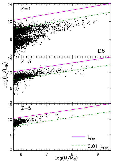
Figure 1: Relation between mass and bolometric luminosity for black holes in the D6 simulation for redshifts 1, 3, and 5. The lines show $\rm{L_{Edd}}$ (solid pink) and $\rm{0.01L_{Edd}}$ (dashed green).

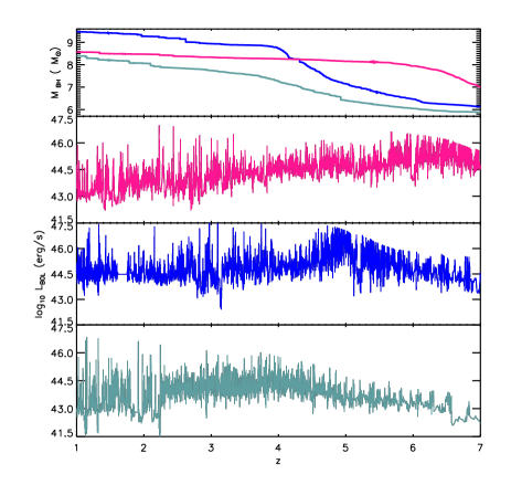
Figure 2: Example of lightcurves between z=1 and z=7 for three massive black holes in the D6 simulation. The top panel shows the growth of the black hole masses and bottom three panels (in corresponding colors) show the associated lightcurves for their bolometric luminosity.

3 Results

3.1 Mass-Luminosity Relation

In order to illustrate the range of properties of the black hole population in the simulations, in Fig. 1 we show the relation between black hole mass and luminosity for the whole sample of objects in the D6 simulation (at $z=1,3,\>\rm{and}\>5$). Note the D4 and E6 mass-luminosity relations are not plotted, but both produced similar results. There is some correlation, albeit weak, between luminosity and mass of black holes, however in most regimes a significant scatter is seen, implying a fair range of luminosities for a fixed black hole mass. This is the direct result of our simulations and in particular the complex lightcurves associated with the accretion history (and the evolution of the gas supply) which is followed in detail for all the black holes in our simulations. As an example, in Fig. 2 we show the black hole mass assembly history for three specific black holes in the D6 simulations and their associated lightcurves (in terms of bolometric luminosity). The high level of variability in the lightcurves is induced by the detailed hydrodynamics, interplay between gas inflows, associated accretion and feedback processes self-consistently modelled in the simulations (see also Di Matteo et al. (2008) for more examples of accretion and merger histories of black holes in the simulations). This implies that in turn we expect the same black holes, at different stages of activity, to contribute to different regions of the luminosity function.

3.2 Luminosity Functions

To illustrate the effect of different black hole populations to the QLF in detail, in Figure 3 we plot the relative contribution from the different black hole mass ranges to the luminosity function at $z=1$ and 3. At $z=1$, the black holes with mass below $10^{7}M_{\odot}$ provide the dominant contribution to the luminosity function for luminosities below $10^{9.5}L_{\odot}(10^{43}\rm{erg}\>\rm{s}^{-1})$, while higher masses dominate at larger luminosities. At higher redshift, the low mass black holes are the dominant contribution up to a higher luminosity ($10^{10.5}L_{\odot}$ at $z=3$), and have a more significant contribution to higher luminosities than they do at low redshift. Note that black holes with masses $<10^{7}M_{\odot}$ give rise to a significant steepening of the luminosity function below $\sim 10^{10}L_{\odot}$ (although this is sometimes below the current observational limits, it is an important effect in our results). In our numerical simulations we do not expect to resolve the accretion history on to the lowest mass black holes (as also shown by increased scatter in Fig. 1), where the gas dynamics are well resolved only well beyond the black hole accretion radius. For this reason, as well as the fact that the low-mass black holes correspond primarily to recently inserted seed particles which have yet to undergo critical accretion phases (i.e. dependent on our initial choice of this parameter), we will use only black holes with $M_{\rm BH}>10^{6}M_{\odot}$ for the rest of our analysis.

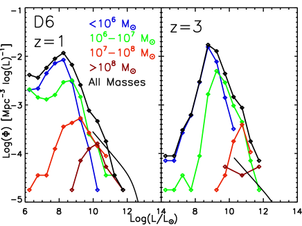
Figure 3: The luminosity function as computed for the D6 simulation at redshifts 1 and 3 for black holes restricted to the following ranges: Blue: $<10^{6}M_{\odot}$; Green: $10^{6}-10^{7}M_{\odot}$; Red: $10^{7}-10^{8}M_{\odot}$; Brown: $>10^{8}M_{\odot}$; Black: Full mass range. The Hopkins et al. (2007b) best-fitting bolometric QLF has also been plotted for comparison (Solid black line).

Fig. 4 shows the predictions from our simulations for the AGN luminosity functions for $z=0.5,1,2,3,4,5$, (note that only the D4 simulation is used at $z=0.5$). The first column shows the bolometric luminosity function derived directly from the simulations. The second and third columns show the luminosity function after applying the bolometric correction (Eq.1) to obtain the B-band (second column) and 2-10 keV hard X-ray band (third column) QLFs. Along with our predictions, we plot the observational data and the best-fitting QLFs from several studies for the hard X-ray and optical bands (see Fig. 4 caption for complete list of references).

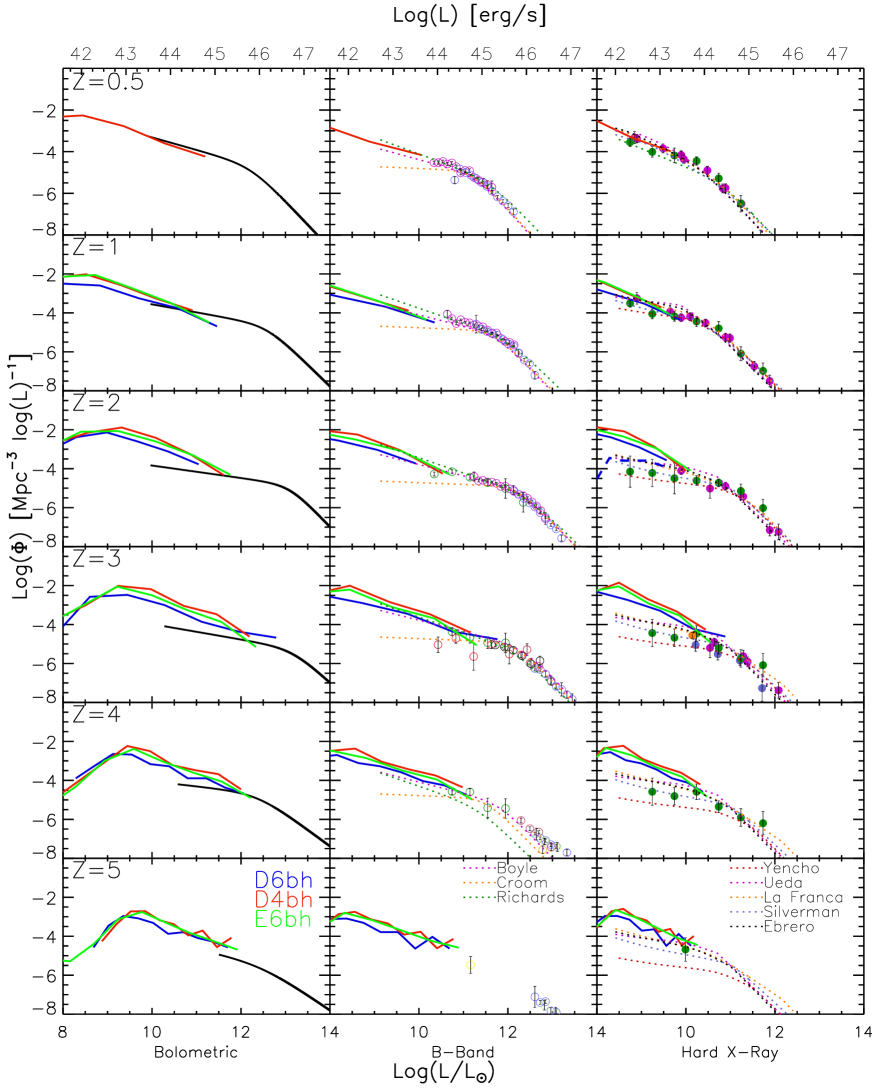
Figure 4: The black hole luminosity function for all three simulations (blue - D6 simulation; red - D4 simulation; green - E6 simulation) using sources with $M_{\rm BH}>10^{6}M_{\odot}$. The first column is the bolometric QLF computed directly from the simulation. The solid black line is the double-power law QLF function given in Hopkins et al. (2007b). The second and third columns show the luminosity function after applying a bolometric correction (Eq. 1) to produce the B-Band and Hard X-ray band. Open circles for optical bands are datapoints from the following studies: Bright purple - Richards et al. (2005); Blue - Richards et al. (2006); Dark Green - Wolf et al. (2003); Red - Hunt et al. (2004); Yellow - Cristiani et al. (2004); Orange - Kennefick et al. (1995); Dark Purple - Schmidt et al. (1995); Bright Green - Fan et al. (2001a, b, 2003, 2004); Black - Siana et al. (2006). Closed circles for hard X-ray bands are datapoints from the following studies: Pink - Ueda et al. (2003); Blue - Silverman et al. (2005); Green - Barger et al. (2005, 2003a, 2003b); Orange - Nandra et al. (2005). Dotted lines in the hard X-ray column are best-fitting LDDE functions from the following studies: Pink - Ueda et al. (2003); Orange - La Franca et al. (2005); Purple - Silverman et al. (2008); Black - Ebrero et al. (2009); Red - Yencho et al. (2009). Dotted lines in the B-Band column are best-fitting LDDE functions from the following studies: Pink - Boyle et al. (2000); Orange - Croom et al. (2004); Green - Richards et al. (2005). The dashed line in the hard X-ray at z=2 is the D6 QLF if only $M_{\rm BH}>10^{7.5}M_{\odot}$ are included.

The bolometric luminosities are compared to the best-fitting function computed by Hopkins et al. (2007b) who compiled all available data from observational studies across several bands, including the optical, mid-infrared, hard and soft X-ray bands, and fitted them to a double power law function (see Hopkins et al. (2007b) for the function and the table of redshift-dependent parameters). The best-fitting function is plotted consistent with the range of observed bolometric luminosities. This is why the minimum luminosity shown in these fit functions is redshift-dependent, and ranges from $9.97L_{\odot}$ at z=1 to $11.53L_{\odot}$ at z=6.

Comparing observed and predicted LFs, it is apparent that the simulations can only reproduce the ’faint-end’ of the LF: this is expected as the number density of AGNs in the ’bright-end’ is simply too low to be accessible in our simulated volumes. Thus our predictions are limited to a relatively small range of luminosities which can be compared directly to observational data, and the largest overlap is in the X-ray band, rather than in the B-band due to the significantly fainter AGN populations in the former. Related to this is the lack of predictions for the knee of the QLF, which occurs at a higher luminosity than the simulations produce.

Within the range of comparison, our predictions agree well with the data. Our simulations are fully consistent with the constraints from the B-band (albeit with very limited region of overlap). In the hard X-ray band, at $L\sim 10^{10}\L_{\odot}$ ($L\sim 10^{43.5}$ erg s^-1), close to the maximum luminosities probed with our simulations, there is also very good agreement. For $z\leq 1$ the overall shape and slope of the faint-end is also reproduced remarkably well. At $2\leq z\leq 4$ however, the slope predicted from the simulation is typically steeper than in the observed LFs. At $z>4$, if compared to the fits of the observations, the slopes are again consistent. The same result is found in the comparison with the bolometric luminosity functions (where indeed the hard X-ray data significantly dominates Hopkins’ fits in the low luminosity end) and where the discrepancy in the slope is the greatest at $z\sim 2$.

It is promising that the simulations agree well with the data at $z\leq 1$ where the observations in the ’faint-end’ are most complete and the bolometric corrections (which are derived from the local samples and have no redshift dependence) are most appropriately applied. The larger number of AGNs at the faintest luminosities (hence the steeper slopes) at higher redshifts may have two possible implications. One is that there is still a population of the faint, possibly heavily obscured AGN above $z=2$ that have not yet been detected. Alternatively, our simulations are actually overproducing the faint AGN population due to lack of appropriate resolution or appropriate feedback physics (either due to stellar processes or AGN) in the faint, low mass black hole population. The latter possibility is also hinted at from our results in Fig. 3 and the fact that the D6 predictions (highest resolution simulation) typically predict the flattest slopes (albeit barely as the convergence between the predictions for the three simulations is good). We will investigate this further in the course of the paper.

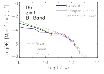
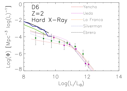
Figure 5: The QLF for D6 simulation for B-Band at z=1 (left) and Hard X-ray at z=2 (right) using different model parameters: Black - same parameters as Fig. 4; Blue - sources with $\rm{L}>\rm{0.01L_{Edd}}$; Green - luminosity-independent bolometric correction. See Fig. 4 for references of observational datapoints and best-fitting functions.

3.2.1 Model dependent effects on the predictions for QLF

Even though our simulations predict directly an accretion rate for each of the BHs (from the hydrodynamics), at any given time there are two major model dependent assumptions that we have made in order to the translate the accretion rate into a luminosity in a particular waveband: one is the assumption of a fixed radiative efficiency of ten per cent, and the second is the use of an empirically derived bolometric correction. Here we wish to investigate the main effects on the QLF predictions of varying these two assumptions. In Figure 5 we demonstrate these effect by showing the B-Band QLF at z=1 (left) and the hard X-ray band QLF at z=2 (right). With these two panels we are able to fully illustrate the relevance of the effects.

When calculating black hole luminosities (as described in Section 2.1), we are assuming that all sources have equal radiative efficiency and set it to 0.1. However, it has been suggested (even though the precise changes in accretion physics at low accretion rate remain somewhat uncertain) that sources accreting at a sufficiently low Eddington fraction (typically at $\approx 0.01$ Eddington) are expected to transition to a radiatively inefficient state with associated changes in the spectral energy distribution (SED) that are dramatically different. These radiatively inefficient accretion models (e.g. Narayan, 2005; Quataert & Narayan, 1999; Yuan & Narayan, 2004, and references therein) (and also observations of both AGN and X-ray transients) indicate that such transitions occur around accretion rates of 1% the Eddington value. The simplest way to investigate the overall effect this may have on our QLF predictions is to eliminate all sources accreting below $0.01\rm{L_{Edd}}$ (blue line). As shown in Figure 1, most sources are above this cut-off luminosity at $z>1$, so we expect a minimal effect on the QLF above this redshift. Eliminating low luminosity sources for $z\leq 1$ leads to a flattening of the QLF slope (Fig. 5), as most sources are actually below this threshold at this point (as indeed generally expected that such modes of accretion will be well below the quasar peak). In short, low radiative efficiency accretion is expected to lead to some flattening of the QLF at $z\leq 1$. This effect therefore would not help flattening the QLF function at higher redshift and therefore better reconcile our predictions with observations.

Our predictions for the various wavebands are of course dependent on the form of the bolometric correction used (the one adopted here is shown in Eq. 1). Even though there is a luminosity dependence in our bolometric correction, it is less well-constrained at low luminosities (also for the reasons discussed above), where the majority of our sources lie. To explore the effects that the luminosity dependence has on our results in Figure 5 (green line) we show the QLFs for a luminosity-independent bolometric correction, using the value of the correction factor evaluated at $L=10^{12}L_{\odot}$, where the correction factor is best constrained. Doing this has a small effect on the B-Band QLF, where in any case (see Eq.1) the correction has a small dependence on luminosity. In the hard X-ray band, however, a luminosity independent correction produces significantly lower magnitude for the QLF, which more closely matches the observational data. This illustrates that the exact form of the bolometric correction, particularly the form of its luminosity dependence, may have a strong effect on our final results.

3.3 Comoving Number Density Evolution

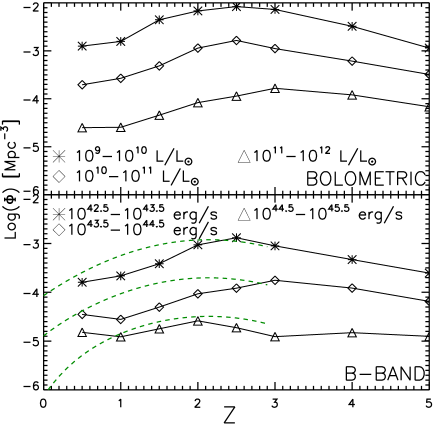
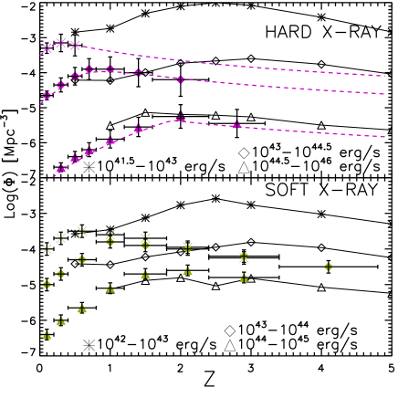
Figure 6: The comoving number density evolution of quasars for $M_{\rm BH}>10^{6}M_{\odot}$ averaged across the three simulations (except at $z=0.5$, where only the D4 simulation was available). A linear extrapolation has been applied to the simulation to allow our luminosity function to be integrated over the given luminosity ranges, and be compared directly to observational data from Ueda et al. (2003) (hard X-ray - purple triangles) and Hasinger et al. (2005) (soft X-ray - green triangles). We have also plotted the predictions from the best-fitting functions from Richards et al. (2005) (optical - green dashed line) and Ueda et al. (2003) (hard X-ray - purple dashed line). Note the optical observational data were limited to redshifts below $z=3$, so we have only plotted those curves for $z<3$. Additionally, the soft X-ray data have been adjusted for obscuration as in Hopkins et al. (2006b).

The quasar comoving number density evolution is plotted in Fig. 6. This is derived by integrating the luminosity functions plotted in Fig. 4 (we average over all three simulations). Again we plot the predictions for the bolometric, B-band, hard X-ray and in this case soft X-ray band also. For the latter two bands we also show the observational constraints from Ueda et al. (2003) (hard X-ray) and Hasinger et al. (2005) (soft X-ray). Note that, following Hopkins et al. (2006b), the normalization of the soft x-ray data has been multiplied by 10 to adjust for obscuration in this band (this adjustment is somewhat model dependent, but provides a first approximation for comparison). We have also plotted the predictions from the best-fitting functions of Richards et al. (2005) (B-Band) and Ueda et al. (2003) (Hard X-ray). The B-Band function is terminated at $z=3$ since the fits were based only on sources below this redshift. In some cases a linear extrapolation (to higher luminosities) was applied to the simulation to allow the range of integration to match the observational data (given in specific luminosity bins).

In virtually every band, the quasar number density from the simulations peaks at $z\sim 2.5$ and as expected, their number density is dominated by the lower luminosity populations. When comparing to the X-ray data (both hard and soft bands), we again find there is good agreement with the observed evolution in the intermediate/high luminosity ranges. Consistent with the results from the luminosity functions, the evolution in the lowest luminosity range implies larger number densities in the soft X-ray band above $z\geq 2$. The hard X-ray data from Ueda et al. (2003) for the lowest luminosity range is limited to $z<0.5$, preventing direct comparison, however the best-fitting function’s extrapolation shows that we may have a similar overestimate for the hard X-ray band.

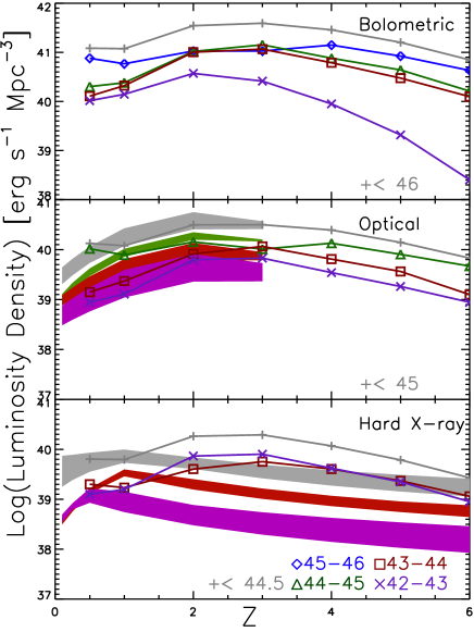
Figure 7: The total luminosity density evolution averaged across the three simulations (except at $z=0.5$ where only the D4 simulation was used). Top panel - bolometric prediction computed directly from simulation; remaining plots - optical and hard X-ray predictions obtained by applying bolometric corrections to the bolometric luminosities. Grey crosses show the luminosity density evolution below a certain cutoff luminosity (chosen at approximately the lowest break luminosity for the given band to restrict our predictions to the faint-end). The remaining (colored) symbols show the emissivity produced by black holes within the following luminosity ranges: Blue diamonds - $10^{45}\>\rm{erg}\>s^{-1}<L<10^{46}\>\rm{erg}\>s^{-1}$; Green triangles - $10^{44}\>\rm{erg}\>s^{-1}<L<10^{45}\>\rm{erg}\>s^{-1}$; Red squares - $10^{43}\>\rm{erg}\>s^{-1}<L<10^{44}\>\rm{erg}\>s^{-1}$; Purple X - $10^{42}\>\rm{erg}\>s^{-1}<L<10^{43}\>\rm{erg}\>s^{-1}$. The shaded regions are the areas bounded by the best-fitting LDDE functions from Ueda et al. (2003), La Franca et al. (2005) and Ebrero et al. (2009) for hard X-ray and for optical, Richards et al. (2005) and Boyle et al. (2000). Note the observational estimates for the optical band are only plotted for $z<3$ since the observational data was limited to low redshifts.

3.4 Luminosity Density Evolution

In Fig. 7, we show the total luminosity density evolution from the simulated quasars with the appropriate observational constraints. A linear extrapolation of the QLF was made for the highest luminosity bins such that consistent luminosity ranges could be used across all simulations and redshifts. To cover the full range of observational constraints, we have used the best-fitting luminosity-dependent density evolution (LDDE) functions from the following studies to bound the shaded regions: in optical - Richards et al. (2005) and Boyle et al. (2000); in hard X-ray - Ueda et al. (2003), La Franca et al. (2005) and Ebrero et al. (2009). For these reasons, Fig. 7 is less of a direct comparison between simulations (where we extrapolate somewhat) and observations (where we used model dependent fits to data as constraints).

While the predicted peak in the total luminosity density is at $z\sim 2.5$ across the various bands, there are some fairly marked differences in the objects that dominate the contribution to the total luminosity evolution. The bolometric luminosity density (top panel) is dominated by the highest luminosity bins, with the brightest objects peaking at $z\sim 4$ while the lower luminosity bins peak at $z\sim 2$. In the optical band (second panel), the luminosity density is still dominated by the brightest objects, comparable to the observational constraints.

The most significant difference is in the X-ray band, where the low luminosity population produces most of the contribution to the luminosity density. Additionally, the peak in observed luminosity density is close to $z\sim 1$ rather than $z\sim 2.5$ as implied by the simulations. The overall reversal of trends in the relative contributions in various bands is of course caused by the form of the bolometric correction used in Eq. 1.

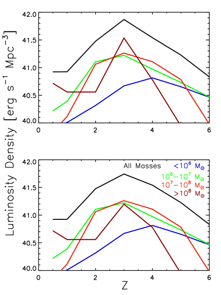
Figure 8: The total bolometric luminosity density evolution averaged across the three simulations (except at $z=0.5$ where only the D4 simulation was run), broken into mass bins. The upper plot includes all black holes, while the lower plot has neglected the outlying black hole in the D6 simulation at redshift 3.

Finally, Fig. 8 shows the contribution to the bolometric luminosity density evolution as a function of black hole mass. The lower plot in Fig. 8 is identical to the upper plot except the single most luminous black hole from the D6 simulation at redshift 3 has been neglected (to explicitly show effects due to small statistics). We find that it is typically the midrange black holes masses ($10^{6}M_{\odot}<M_{\rm BH}<10^{8}M_{\odot}$) which provide the largest contribution to the luminosity density. As one might expect, at higher redshifts, the low mass black holes provide a more significant contribution, which was expected due to the lack of high mass black holes (see also Fig. 1).

4 Discussion

One of our primary results from the luminosity function and the global number density and luminosity density evolution is that our simulations are in good agreement with the observational constraints but imply a larger number of low luminosity X-ray sources (at $z>2$) than observed. In order to assess the viability of our results we need to check whether this population may violate the current constraints on the total X-ray background (XRB). The XRB intensity is calculated according to (Peacock, 1999)

$$I_{\nu}=\frac{c}{4\pi H_{0}}\int^{z_{2}}_{z_{1}}\epsilon_{\nu}([1+z]\nu_{0},z)\frac{dz}{(1+z)^{2}\sqrt{(1+\Omega_{0}z)}}$$ (2)

where the emissivity, $\epsilon_{\nu}$ is the hard X-ray emissivity shown in Fig. 7, $z$ is the redshift, [$z_{1},z_{2}$] is the range of redshifts being considered, $\nu_{0}$ is the frequency at redshift zero, $H_{0}$ is the Hubble Parameter at redshift zero, and $\Omega_{0}$ is the total density parameter at redshift zero. A photon index of $\Gamma=1.8$ was assumed when computing $\epsilon_{\nu}([1+z]\nu_{0})$ to account for the form of the power spectrum of the black holes. Since we only have simulation information at discrete redshifts, we interpolate $\epsilon_{\nu}$ linearly between datapoints to compute the integral.

We find that the total contribution to the 2-10 keV X-ray background from our simulated black holes is $I_{2-10{\rm keV,D6}}=1.28\times 10^{-11}\rm{erg\>s^{-1}cm^{-2}deg^{-2}}$ for the D6 simulation (recall the simulations are restricted to $z\geq 1$). This is well within the observed 2-10 keV hard X-ray background intensity, $I_{2-10{\rm keV,obs}}=2.02\pm 0.11\times 10^{-11}\rm{erg\>s^{-1}cm^{-2}deg^{-2}}$ (Moretti et al., 2003). If we apply a linear extrapolation to the simulation to include an approximate contribution from $z<1$, we predict a total XRB intensity of $I_{2-10{\rm keV}}=1.8\times 10^{-11}\rm{erg\>s^{-1}cm^{-2}deg^{-2}}$, still below the observed value.

When we do a similar calculation using the E6 and D4 simulations (which have lower resolution) we produce XRB intensities of $I_{2-10{\rm keV}}=1.94\times 10^{-11}$ and $2.87\times 10^{-11}\rm{erg\>s^{-1}cm^{-2}deg^{-2}}$ for the E6 and D4 simultions at $z>1$, respectively. With the D4 simulation we are starting to violate the observed XRB even without including $z<1$. This result is quite fundamental for our analysis as it indicates that the simulation resolution plays an important role in estimating the effect from the faintest sources (those that were found to be in excess of the observed LF) and that their contribution decreases with higher resolution (note in Fig. 4 the steepest slopes of LF are always predicted from the D4 run).

Our simulations also predict that the QLFs extend to fainter fluxes than currently observed. We therefore compare our predictions for the unresolved fraction of the 2-8 keV XRB from the D6 simulation to test whether current observational constraints are still consistent with our predictions (i.e. if we could still be missing a faint population of e.g. heavily obscured AGN). We found that our prediction for the XRB contribution from luminosities limited to the range of overlap between observation and simulation provides an excess intensity of $1.85\times 10^{-12}\rm{erg\>s^{-1}cm^{-2}deg^{-2}}$ in the 2-8 keV band (assuming photon index of 1.8). This is below the 2-8 keV unresolved background of $I_{2-8{\rm keV,unres}}=3.4\pm 1.7\times 10^{-12}\rm{erg\>s^{-1}cm^{-2}deg^{-2}}$ (Hickox & Markevitch, 2006). If we take into account the total contribution from the whole population in the simulations (well below the faintest sources currently observed but still assuming the same X-ray spectrum) we are in excess of the unresolved background by almost a factor of 2. To further illustrate and elucidate this issue, in Fig. 9 we plot the differential contribution to the 2-10 keV background from the simulations and the observations in several redshift bins (the filled curves are the regions bounded by the predictions from Ueda et al. (2003), La Franca et al. (2005) and Ebrero et al. (2009)). This shows again that the excess in our predictions is caused by the contribution from low-luminosity sources ($L<10^{43}\rm{erg\>s^{-1}}$) and originates mostly at $z\geq 2$. This supports the idea that the faintest sources at high redshift are problematic in our predictions. Figs. 3 and 7 do indeed show that above z=2 this population is dominated by the lowest mass black holes (as opposed to lower redshifts where a more significant fraction of high mass black holes have ’turned-off’) and those that are likely to suffer more strongly from lack of resolution. For illustration, in Fig. 4, at z = 2, in the hard X-ray band we show how the predictions look when only $M_{\rm BH}>10^{7.5}M_{\odot}$ are plotted. The excess in our prediction is eliminated and the lowest luminosity end of the LF is now in good agreement with all the observations.

Note also that we have used a redshift-independent correction to convert the simulations’ bolometric luminosity to the hard X-ray band to compare with observations. Direct determinations of bolometric the correction as a function of redshift are not yet available and this may further bias our results at $z\geq 2$.

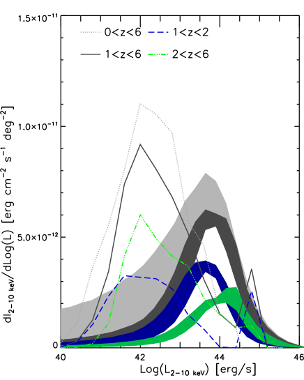
Figure 9: The differential contribution to the 2-10 keV hard X-ray background intensity as a function of luminosity, plotted for several redshift bins. The shaded areas show the region of contributions bounded by the predictions by Ueda et al. (2003), La Franca et al. (2005) and Ebrero et al. (2009). The dotted line is an extrapolation of the simulation obtained by extending the luminosity density evolution from $z=1$ to $z=0$.

5 Conclusions

Here we study the luminosity function and its evolution for populations of quasars extracted from full cosmological hydrodynamical simulations which include direct modelling for the growth of black holes. Noting that our simulations (due to limitations on the volumes probed) can only be used to study the faint-end of the QLF, we summarize our main results as follows:

• Consistent with the complex light-curves and various phases of activity that black holes undergo through their cosmic history, we have shown that there is a significant spread in luminosities for a given black hole mass, and in turn that different black hole masses contribute to the same regions of the QLF.

• At low redshift ($z<2$), the low luminosity ranges (below $10^{9}L_{\odot}$) of the QLF are dominated by black holes below $10^{7}M_{\odot}$, while the luminosities above $10^{9}L_{\odot}$ contain comparable contributions from both low and high masses. At high redshift the majority of black holes are below $10^{7}M_{\odot}$, and thus the entire QLF is dominated by low black hole mass sources.

• We have shown that our predictions for the faint-end of the QLF agree remarkably well with observations at $z\leq 1$, but produce steeper slopes than implied by current constraints for the hard X-ray band at redshifts $z=2$ and 3.

• Taking into account a possible transition to low radiative efficiency accretion modes for low accretion rate sources tends to flatten the QLF at low redshifts but this does not affect significantly any of our results.

• The exact form of the bolometric correction has a significant effect on our predictions. In particular, when comparing to a fixed correction, the empirically determined (Eq. 1) luminosity dependence leads to a larger QLF magnitude in the X-ray band. Note also that in addition, no constraints are currently available on the redshift dependence of the correction.

• The evolution of the comoving number density is in agreement with current constraints for the luminosity ranges above $10^{43}\rm{erg\>s^{-1}}$. Agreement for luminosities below $10^{43}\rm{erg\>s^{-1}}$ is significantly worse, but the more limited observational data at these ranges combined with the dominance of black holes with $M_{\rm BH}<10^{7}M_{\odot}$, which are less-well resolved in our simulation makes these results less meaningful.

• The luminosity density evolution predicts a peak luminosity density at $z=2.5$, with comparable contributions from different luminosity bins.

• Based on the slope of the faint-end QLF, the luminosity density evolution and a moderate excess in the unresolved X-ray background, it appears that our simulations are overproducing low luminosity sources, particularly at intermediate redshifts. We have shown however that the higher resolution simulations produce fewer low-luminosity black holes, which makes it likely that this overproduction is dominated by resolution effects. Additionally, our results are most accurate at low redshift, when the high mass (and thus least likely to be affected by resolution limits) sources are most important, further suggesting that our overproduction of low luminosity sources is dominated by resolution effects.

  Overall our results support the interpretation of the faint-end luminosity function put forward by Hopkins et al. In upcoming work we will compare detailed characteristics of black hole lightcurves in our simulations and compare their instantaneous luminosities to their peak luminosities, so as to determine more precisely if the faint-end slope is dominated by quasars radiating below their peak, or by quasars with faint peak luminosities, as previous models assumed. It may be possible (although currently infeasible due to technological constraints) to run larger volume simulations at similar or higher resolution to increase the statistics at the bright-end of the luminosity function and further investigate the rapid dropoff in comoving number density at $z<1$ found in the observational data.

References

- Barger et al. (2003a) Barger A. J., Cowie L. L., Capak P., et al., 2003a, AJ, 126, 632
- Barger et al. (2003b) Barger A. J., Cowie L. L., Capak P., et al., 2003b, ApJL, 584, L61
- Barger et al. (2005) Barger A. J., Cowie L. L., Mushotzky R. F., et al., 2005, AJ, 129, 578
- Begelman et al. (2006) Begelman M. C., Volonteri M., Rees M. J., 2006, MNRAS, 370, 289
- Bondi (1952) Bondi H., 1952, MNRAS, 112, 195
- Bondi & Hoyle (1944) Bondi H., Hoyle F., 1944, MNRAS, 104, 273
- Bonoli et al. (2009) Bonoli S., Marulli F., Springel V., White S. D. M., Branchini E., Moscardini L., 2009, MNRAS, 606
- Bower et al. (2006) Bower R. G., Benson A. J., Malbon R., et al., 2006, MNRAS, 370, 645
- Boyle et al. (2000) Boyle B. J., Shanks T., Croom S. M., et al., 2000, MNRAS, 317, 1014
- Brown et al. (2006) Brown M. J. I., Brand K., Dey A., et al., 2006, ApJ, 638, 88
- Burkert & Silk (2001) Burkert A., Silk J., 2001, ApJL, 554, L151
- Churazov et al. (2005) Churazov E., Sazonov S., Sunyaev R., Forman W., Jones C., Böhringer H., 2005, MNRAS, 363, L91
- Ciotti & Ostriker (2007) Ciotti L., Ostriker J. P., 2007, ApJ, 665, 1038
- Cirasuolo et al. (2005) Cirasuolo M., Magliocchetti M., Celotti A., 2005, MNRAS, 357, 1267
- Cowie et al. (2003) Cowie L. L., Barger A. J., Bautz M. W., Brandt W. N., Garmire G. P., 2003, ApJL, 584, L57
- Cristiani et al. (2004) Cristiani S., Alexander D. M., Bauer F., et al., 2004, ApJL, 600, L119
- Croom et al. (2004) Croom S. M., Smith R. J., Boyle B. J., et al., 2004, MNRAS, 349, 1397
- Croton et al. (2006) Croton D. J., Springel V., White S. D. M., et al., 2006, MNRAS, 365, 11
- Di Matteo et al. (2008) Di Matteo T., Colberg J., Springel V., Hernquist L., Sijacki D., 2008, ApJ, 676, 33
- Di Matteo et al. (2005) Di Matteo T., Springel V., Hernquist L., 2005, Nature, 433, 604
- Ebrero et al. (2009) Ebrero J., Carrera F. J., Page M. J., et al., 2009, A&A, 493, 55
- Fan et al. (2004) Fan X., Hennawi J. F., Richards G. T., et al., 2004, AJ, 128, 515
- Fan et al. (2001a) Fan X., Narayanan V. K., Lupton R. H., et al., 2001a, AJ, 122, 2833
- Fan et al. (2001b) Fan X., Strauss M. A., Schneider D. P., et al., 2001b, AJ, 121, 54
- Fan et al. (2003) Fan X., Strauss M. A., Schneider D. P., et al., 2003, AJ, 125, 1649
- Ferrarese & Merritt (2000) Ferrarese L., Merritt D., 2000, ApJL, 539, L9
- Fiore et al. (2003) Fiore F., Brusa M., Cocchia F., et al., 2003, A&A, 409, 79
- Gebhardt et al. (2000) Gebhardt K., Bender R., Bower G., et al., 2000, ApJL, 539, L13
- Graham & Driver (2007) Graham A. W., Driver S. P., 2007, ApJ, 655, 77
- Granato et al. (2004) Granato G. L., De Zotti G., Silva L., Bressan A., Danese L., 2004, ApJ, 600, 580
- Haiman et al. (2004) Haiman Z., Quataert E., Bower G. C., 2004, ApJ, 612, 698
- Hasinger et al. (2005) Hasinger G., Miyaji T., Schmidt M., 2005, A&A, 441, 417
- Hickox & Markevitch (2006) Hickox R. C., Markevitch M., 2006, ApJ, 645, 95
- Hopkins et al. (2005a) Hopkins P. F., Hernquist L., Cox T. J., et al., 2005a, ApJ, 630, 705
- Hopkins et al. (2005b) Hopkins P. F., Hernquist L., Cox T. J., Di Matteo T., Robertson B., Springel V., 2005b, ApJ, 630, 716
- Hopkins et al. (2006a) Hopkins P. F., Hernquist L., Cox T. J., Di Matteo T., Robertson B., Springel V., 2006a, ApJS, 163, 1
- Hopkins et al. (2006b) Hopkins P. F., Hernquist L., Cox T. J., Robertson B., Di Matteo T., Springel V., 2006b, ApJ, 639, 700
- Hopkins et al. (2007a) Hopkins P. F., Hernquist L., Cox T. J., Robertson B., Krause E., 2007a, ApJ, 669, 45
- Hopkins et al. (2005c) Hopkins P. F., Hernquist L., Martini P., et al., 2005c, ApJL, 625, L71
- Hopkins et al. (2007b) Hopkins P. F., Richards G. T., Hernquist L., 2007b, ApJ, 654, 731
- Hoyle & Lyttleton (1939) Hoyle F., Lyttleton R. A., 1939, in Proceedings of the Cambridge Philosophical Society, vol. 35 of Proceedings of the Cambridge Philosophical Society, 405
- Hunt et al. (2004) Hunt M. P., Steidel C. C., Adelberger K. L., Shapley A. E., 2004, ApJ, 605, 625
- Kauffmann & Haehnelt (2000) Kauffmann G., Haehnelt M., 2000, MNRAS, 311, 576
- Kawata & Gibson (2005) Kawata D., Gibson B. K., 2005, MNRAS, 358, L16
- Kennefick et al. (1995) Kennefick J. D., Djorgovski S. G., de Carvalho R. R., 1995, AJ, 110, 2553
- Kormendy & Richstone (1995) Kormendy J., Richstone D., 1995, ARA&A, 33, 581
- La Franca et al. (2005) La Franca F., Fiore F., Comastri A., et al., 2005, ApJ, 635, 864
- La Franca et al. (2002) La Franca F., Fiore F., Vignali C., et al., 2002, ApJ, 570, 100
- Lewis et al. (2002) Lewis I. J., Cannon R. D., Taylor K., et al., 2002, MNRAS, 333, 279
- Magorrian et al. (1998) Magorrian J., Tremaine S., Richstone D., et al., 1998, AJ, 115, 2285
- Malbon et al. (2007) Malbon R. K., Baugh C. M., Frenk C. S., Lacey C. G., 2007, MNRAS, 382, 1394
- Marconi et al. (2004) Marconi A., Risaliti G., Gilli R., Hunt L. K., Maiolino R., Salvati M., 2004, MNRAS, 351, 169
- Marulli et al. (2008) Marulli F., Bonoli S., Branchini E., Moscardini L., Springel V., 2008, MNRAS, 385, 1846
- Matute et al. (2006) Matute I., La Franca F., Pozzi F., Gruppioni C., Lari C., Zamorani G., 2006, A&A, 451, 443
- Miyaji et al. (2001) Miyaji T., Hasinger G., Schmidt M., 2001, A&A, 369, 49
- Moretti et al. (2003) Moretti A., Campana S., Lazzati D., Tagliaferri G., 2003, ApJ, 588, 696
- Nandra et al. (2005) Nandra K., Laird E. S., Steidel C. C., 2005, MNRAS, 360, L39
- Narayan (2005) Narayan R., 2005, AP&SS, 300, 177
- Okamoto et al. (2008) Okamoto T., Nemmen R. S., Bower R. G., 2008, MNRAS, 385, 161
- Page et al. (1997) Page M. J., Mason K. O., McHardy I. M., Jones L. R., Carrera F. J., 1997, MNRAS, 291, 324
- Peacock (1999) Peacock J. A., 1999, Cosmological Physics, Cosmological Physics, by John A. Peacock, pp. 704. ISBN 052141072X. Cambridge, UK: Cambridge University Press, January 1999.
- Quataert & Narayan (1999) Quataert E., Narayan R., 1999, ApJ, 520, 298
- Richards et al. (2005) Richards G. T., Croom S. M., Anderson S. F., et al., 2005, MNRAS, 360, 839
- Richards et al. (2006) Richards G. T., Strauss M. A., Fan X., et al., 2006, AJ, 131, 2766
- Sazonov et al. (2004) Sazonov S. Y., Ostriker J. P., Sunyaev R. A., 2004, MNRAS, 347, 144
- Schmidt et al. (1995) Schmidt M., Schneider D. P., Gunn J. E., 1995, AJ, 110, 68
- Shakura & Sunyaev (1973) Shakura N. I., Sunyaev R. A., 1973, A&A, 24, 337
- Siana et al. (2006) Siana B., Polletta M., Smith H. E., et al., 2006, ArXiv Astrophysics e-prints:astro-ph/0604373
- Sijacki et al. (2007) Sijacki D., Springel V., di Matteo T., Hernquist L., 2007, MNRAS, 380, 877
- Silverman et al. (2005) Silverman J. D., Green P. J., Barkhouse W. A., et al., 2005, ApJ, 618, 123
- Silverman et al. (2008) Silverman J. D., Green P. J., Barkhouse W. A., et al., 2008, ApJ, 679, 118
- Springel et al. (2005a) Springel V., Di Matteo T., Hernquist L., 2005a, ApJL, 620, L79
- Springel et al. (2005b) Springel V., Di Matteo T., Hernquist L., 2005b, MNRAS, 361, 776
- Tremaine et al. (2002) Tremaine S., Gebhardt K., Bender R., et al., 2002, ApJ, 574, 740
- Treu et al. (2007) Treu T., Woo J.-H., Malkan M. A., Blandford R. D., 2007, ApJ, 667, 117
- Ueda et al. (2003) Ueda Y., Akiyama M., Ohta K., Miyaji T., 2003, ApJ, 598, 886
- Volonteri et al. (2003) Volonteri M., Haardt F., Madau P., 2003, ApJ, 582, 559
- Wall et al. (2005) Wall J. V., Jackson C. A., Shaver P. A., Hook I. M., Kellermann K. I., 2005, A&A, 434, 133
- Wolf et al. (2003) Wolf C., Wisotzki L., Borch A., Dye S., Kleinheinrich M., Meisenheimer K., 2003, A&A, 408, 499
- Wyithe & Loeb (2003) Wyithe J. S. B., Loeb A., 2003, ApJ, 595, 614
- Yencho et al. (2009) Yencho B., Barger A. J., Trouille L., Winter L. M., 2009, ApJ, 698, 380
- York et al. (2000) York D. G., Adelman J., Anderson Jr. J. E., et al., 2000, AJ, 120, 1579
- Yuan & Narayan (2004) Yuan F., Narayan R., 2004, ApJ, 612, 724