High Fidelity State Transfer Over an Unmodulated Linear $XY$ Spin Chain

Abstract

We provide a class of initial encodings that can be sent with a high fidelity over an unmodulated, linear, $XY$ spin chain. As an example, an average fidelity of ninety-six percent can be obtained using an eleven-spin encoding to transmit a state over a chain containing ten-thousand spins. An analysis of the magnetic field dependence is given, and conditions for field optimization are provided.

I Introduction

The notion of using an unmodulated spin chain to serve as a channel for the transmission of quantum information was put forth by Bose in 2003 S. Bose (2003). To improve the communication fidelity of the original proposal, a considerable effort has been made in order to find ways of preserving the integrity of a quantum state as it propagates across these quantum wires. It was recently shown that, in principle, perfect state transfer can be obtained between processors that are connected by any interacting media L.-A. Wu, Y. Liu, F. Nori (2009). Specific protocols which yield ideal state transmissions have also been proposed using quantum dots G. M. Nikolopoulos, D. Petrosyan and P. Lambropoulos (2004); G.M. Nikolopoulos, D. Petrosyan, P. Lambropoulos (2004) and spin-chain systems with non-identical couplings between pairs M. Christandl, N. Datta, A. Ekert, and A.J. Landahl (2004); M. Christandl, N. Datta, T.C. Dorlas, A. Ekert, A. Kay, and A.J. Landahl (2005). It has also been shown that the fidelity can be increased if one can dynamically control the first and last pairs of the chain H.L. Haselgrove (2005). In fact, the fidelity can become arbitrarily large using this last method if there is no limit to the number of sequential gates that can be applied D. Burgarth, V. Giovannetti, and S. Bose (2007). Perfect state transfer can also be obtained without prior initialization of the spin medium if one applies end gates to a chain constructed with pre-engineered couplings C. Di Franco, M. Paternostro, and M.S.Kim (2008). Furthermore, the communication can also be improved if the sender encodes the message state over the space of multiple spins rather than only one T.J. Osborne and N. Linden (2004); H.L. Haselgrove (2005); J. Allcock and N. Linden (2009); Wang et al. (2009). (For a nice review of the subject see Ref. S. Bose (2007).)

In Ref. T.J. Osborne and N. Linden (2004), the authors cleverly chose to use the all-spin-down eigenstate to represent the $\left|0\right\rangle$ basis state of an encoded qubit and were able to find single excitation encodings for $\left|1\right\rangle$ that propagated with little dispersion through a spin ring. In their proposal both the sender and receiver have access to multiple spins. They also assumed that the receiver has the ability to unitarily focus the entire probability amplitude of finding the excitation within his region onto a single site. This method can enhance the transfer fidelity to values well above those which can be obtained using the original single spin encoding scheme S. Bose (2003).

Using this protocol Haselgrove derived a method to obtain the initial encodings which maximize the fidelity of state transmission H.L. Haselgrove (2005). His method was based on the singular-value decomposition and can be applied to systems that conserve the total z-component of spin. In particular, his method can be applied to a chain of spin-1/2 particles coupled via the $XY$ interaction. His encodings are optimal in the sense that they maximize the probability amplitude of finding the transmitted excitation somewhere within the receivers accessible region. This is a sufficient condition given the assumption that the receiver can perform the necessary decoding operation mentioned above. In this protocol the fidelity is measured with respect to a single qubit output state although the initial encoding has been carried out using multiple spins.

In Ref. Wang et al. (2009), a particular state was found to transfer well across relatively long $XY$ coupled spin chains. It was shown that if the first and third spins were placed in the singlet state a fidelity of ninety percent or better could be obtained for chains consisting of up to fifty spins. The high fidelities do not depend on the dynamical control of the chain nor do they require the prefabrication of special couplings for each neighboring pair. The fidelities were determined according to the direct overlap between the received state and the actual state which was sent, i.e., the receiver was not required to implement a decoding unitary. Given the assumption that the chain was placed in the all-spin-down ground state prior to initialization, one can reliably transmit information to the receiving end using a simple two spin encoding.

Motivated by this result, we have found a class of effective $k$-qubit encodings ($k=2,3,\ldots$) which can be used to reliably send an encoded qubit state over very long chains. Each member of this class has a structure similar to the singlet encoding of Wang et al. (2009), with each increase in $k$ yielding higher fidelities. We take these states to represent the $\left|1\right\rangle$ basis of a logical qubit, with $\left|0\right\rangle$ taken to be the all-spin-down eigenstate. The paper will focus on the least technically challenging $XY$ configuration; we consider linear arrays of spins having constant and equal exchange couplings between neighboring pairs. As in Wang et al. (2009), we will not require the receiver to implement a decoding operation, we simply let the encoded states propagate freely across the chain. As an example of the reliability of these states, we find that an eleven-qubit encoding can be sent across a chain containing ten-thousand spins and arrive with an average fidelity of ninety-six percent. We analyze the influence of an external magnetic field and find that by isolating the system one can maximize the fidelity provided that the chain has an appropriate number of sites.

We also compare our results to those which can be obtained using Haselgrove’s method. We find that for small chains his optimal states give slightly higher fidelities than ours when the encodings are viewed to take place over the first $r$ spins ($r=3,4,\ldots$) of the chain. However, our encoded states only use a subset of the first $r$ spins, generally $(r+1)/2$ spins are used. If we compare our $n$-spin encoding to Haselgrove’s $n$-spin encoding, our method yields higher fidelities. Again, we emphasize that his fidelities are determined with the assumption that the receiver has applied a decoding operation while for our states no such requirement is necessary. For long chains our encodings actually converge to Haselgrove’s optimal encodings and it is found that the fidelities are equal before and after the decoding process has taken place.

The second section of this paper will provide the necessary background for what follows. In Sec. III we will introduce this class of states and provide examples of the high fidelities which can be obtained when transferring members of this class over long chains. Sec. IV extends the analysis to encoded qubit states and discusses the associated average fidelities. That section also includes a discussion of the dependence of the fidelity on a global magnetic field. In Sec. V we will compare our results to those using Haselgrove’s method. Finally, we will conclude with a summary of our results in Sec. VI.

II Unitary Evolution of a Spin Chain: XY Model

We will consider a linear chain of qubits with uniform, time-independent nearest neighbor couplings. The chain is subjected to a global magnetic field $h$ (aligned along the $z$-axis) which is assumed to remain static over time. The Hamiltonian function of this $N$-spin system is

$$H=-\frac{J}{2}\sum_{i=1}^{N-1}(\sigma_{i}^{x}\sigma_{i+1}^{x}+\sigma_{i}^{y}\sigma_{i+1}^{y})-h\sum_{i=1}^{N}\sigma_{i}^{z},$$ (II.1)

where $\sigma_{i}^{x}$ and $\sigma_{i}^{y}$ are pauli matrices acting on the $i$th spin and $J$ determines the coupling strength.

Following the usual convention, we will let $\left|{\bf{j}}\right\rangle$ $({\bf{j}}={\bf{1,2,...,N}})$ represent the state where all of the spins in the chain point “down” except for the spin at site ${\bf{j}}$ which has been flipped to the “up” state. The ground state will be denoted as $\left|{\bf{0}}\right\rangle=\left|\downarrow\downarrow\downarrow...\downarrow\downarrow\downarrow\right\rangle$. In this paper we will focus strictly on the evolution of states encoded in the Hilbert spaces ${\cal{H}}^{(0)}$ and ${\cal{H}}^{(1)}$, where ${\cal{H}}^{(0)}$ (${\cal{H}}^{(1)}$) are respectively spanned by the states $\{\left|{\bf{0}}\right\rangle\}$ ($\{\left|{\bf{j}}\right\rangle:{\bf{j}}={\bf{1,2,...,N}}\}$). Since the Hamiltonian $H$ (Eq. (II.1)) commutes with $\sum_{i=1}^{N}\sigma_{z}^{i}$, states which are encoded into either space ${\cal{H}}^{(0)}$ or ${\cal{H}}^{(1)}$ will remain there in the absence of noise.

An arbitrary initial encoding over the first $r$ spins of the chain can be expressed in the notation above as

$$\left|{\bf{\Psi}}(0)\right\rangle=\sum_{j=0}^{r}\alpha_{j}\left|{\bf{j}}\right\rangle,$$ (II.2)

with $\sum_{j=0}^{r}|\alpha_{j}|^{2}=1.$ This state evolves unitarily to

$$\left|{\bf{\Psi}}(t)\right\rangle=\alpha_{0}\left|{\bf{0}}\right\rangle+\sum_{j=1}^{N}w_{j}(t)\left|{\bf{j}}\right\rangle,$$ (II.3)

where $w_{j}(t)=\sum_{s=1}^{r}\alpha_{s}\left\langle{\bf{j}}\right|e^{-iHt}\left|{\bf{s}}\right\rangle=\sum_{s=1}^{r}\alpha_{s}f_{s,j}(t).$ (We let $\hbar=1$ throughout.) The transition amplitudes $f_{s,j}(t)$ are given by

$$f_{s,j}(t)=\frac{2}{N+1}\sum_{m=1}^{N}\sin{(q_{m}s)}\sin{(q_{m}j)}e^{-iE_{m}t},$$ (II.4)

with $E_{m}=2h-2J\cos{(q_{m})}$, and $q_{m}=\pi m/(N+1)$.

Given the coefficients $\alpha_{j}$ of an initial encoding along with the transition amplitudes provided in Eq. (II.4) one can calculate the fidelity of state transfer through an unmodulated, linear, XY spin chain. We will provide an expression for the fidelity in the next section and introduce a class of states which travel exceptionally well over a chain composed of a large number of sites.

III High Fidelity Transfer of a Class of States

It was recently shown in Ref. Wang et al. (2009) that an initial encoding of $\left|{\bf{\Psi}}(0)\right\rangle=(\left|{\bf{1}}\right\rangle-\left|{\bf{3}}\right\rangle)/\sqrt{2}$ can be transferred with a relatively high fidelity $(F\approx.9)$ to the opposite end of an unmodulated spin chain containing $N\approx 50$ sites. Since we are assuming that prior to encoding the entire chain has been cooled to its ground state, initializing $\left|{\bf{\Psi}}(0)\right\rangle=(\left|{\bf{1}}\right\rangle-\left|{\bf{3}}\right\rangle)/\sqrt{2}=\frac{\>1}{\sqrt{2}}(\left|\downarrow\uparrow\right\rangle_{1,3}-\left|\uparrow\downarrow\right\rangle_{1,3})\otimes\left|\downarrow\downarrow\downarrow...\downarrow\downarrow\downarrow\right\rangle_{2,4,5,...,N}$ is effectively a two qubit process. This encoding has a very simple structure; with the exception of the singlet placed at the first and third site, every qubit remains in the ground state.

This state belongs to a class of states which consists of effective $k$-qubit encodings ($k=2,3,4,...$) each having a similar structure. We will label the state which corresponds to a specific $k$ as $\left|\Psi_{k}\right\rangle$ and write them explicitly as

$$\left|\Psi_{k}\right\rangle=\frac{\;1}{\sqrt{k}}\sum_{m=0}^{k-1}(-1)^{m}\left|{\bf{2m+1}}\right\rangle,\;\;k=2,3,4,...$$ (III.1)

Each successive increase in $k$ yields a higher fidelity of transmission as the spin chain grows large. To show this let us first express each member of this class in the form $\left|\Psi_{k}\right\rangle=\left|\phi_{k}\right\rangle\otimes\left|\downarrow\downarrow\downarrow...\downarrow\downarrow\downarrow\right\rangle$, where $\left|\phi_{k}\right\rangle$ describes the state of the first $r=2k-1$ spins of the chain. Ideally, at some later time the chain would evolve to $\left|\downarrow\downarrow\downarrow...\downarrow\downarrow\downarrow\right\rangle\otimes\left|\phi_{k}\right\rangle$ in which case a perfect transmission would result. The fidelity between the “encoded” state $\left|\phi_{k}\right\rangle$ and the state corresponding to the last $r$ spins of the chain $\rho(t)$ is given by $F=\sqrt{\left\langle\phi_{k}\right|\rho(t)\left|\phi_{k}\right\rangle}$. Here $\rho(t)$ is the reduced density matrix associated with the state of the receiver’s spins and is obtained by tracing over all but the last $r$ sites of the chain. Since a perfect transmission is described by $\left|\downarrow\downarrow\downarrow...\downarrow\downarrow\downarrow\right\rangle\otimes\left|\phi_{k}\right\rangle$, the state of the first spin of the encoding would ideally propagate to the $[N-(r-1)]{\it{th}}$ site of the chain while the state of the last spin of the encoding (the spin at the $r{\it{th}}$ site) would ideally propagate to the $N{\it{th}}$ site of the chain. For example, when $k=2$ the initial encoding given by $(\left|{\bf{1}}\right\rangle-\left|{\bf{3}}\right\rangle)/\sqrt{2}=(\left|\uparrow\downarrow\downarrow\right\rangle-\left|\downarrow\downarrow\uparrow\right\rangle)/\sqrt{2}\otimes\left|\downarrow\downarrow\downarrow...\downarrow\downarrow\downarrow\right\rangle$ would ideally evolve to the state $\left|\downarrow\downarrow\downarrow...\downarrow\downarrow\downarrow\right\rangle\otimes(\left|\uparrow\downarrow\downarrow\right\rangle-\left|\downarrow\downarrow\uparrow\right\rangle)/\sqrt{2}=(\left|{\bf{N-2}}\right\rangle-\left|{\bf{N}}\right\rangle)/\sqrt{2}$.

In general, the fidelity between an initial encoding given by Eq. (II.2) and the received state can be expressed as

$$F=\sqrt{|G|^{2}+|\alpha_{0}|^{2}\sum_{i=1}^{N-r}|w_{i}|^{2}}$$ (III.2)

where $G=|\alpha_{0}|^{2}+\sum_{i=1}^{r}\alpha_{i}w_{(N-r+i)}^{*}$, and $w_{j}=\sum_{i=1}^{r}\alpha_{i}f_{i,j}(t)$. In this case we have $\alpha_{\nu}=0$ for even $\nu$ and $\alpha_{\nu}=\pm 1/\sqrt{k}$ for odd $\nu$.

Table I lists the maximum fidelity achievable $F$ within the time interval $[0,N]$ along with the associated arrival times $t_{0}$ for the encodings $\left|\Psi_{k}\right\rangle$ ($k=2,3,4,5$). The table shows that as the number of spins grows large the fidelity increases as the value of $k$ increases. We can also see that an increase in the number of spins does not necessarily imply a decrease in the fidelity. In fact, increasing $N$ can actually increase $F$ on occasion, e.g., notice this increase for the states $\left|\Psi_{4}\right\rangle$ and $\left|\Psi_{5}\right\rangle$. Also, for a given number of spins the time in which this maximum fidelity is obtained is nearly equal for neighboring values of $k$.

$k=2$

$N$		100		200		300		400		500		600
$F$		.83		.74		.68		.64		.60		.57
$t_{0}$		51.75		102.36		152.76		203.07		253.33		303.55

$k=3$

$N$		100		200		300		400		500		600
$F$		.90		.88		.84		.81		.78		.75
$t_{0}$		51.08		101.74		152.20		202.55		252.84		303.09

$k=4$

$N$		100		200		300		400		500		600
$F$		.88		.90		.90		.88		.87		.85
$t_{0}$		51.12		101.10		151.54		201.91		252.22		302.49

$k=5$

$N$		100		200		300		400		500		600
$F$		.93		.88		.89		.90		.90		.89
$t_{0}$		51.50		101.22		151.02		201.27		251.56		301.83

Table 1: Table showing the maximum fidelity achievable and the associated arrival times for the states $\left|\Psi_{k}\right\rangle$, $k=2,3,4,5$ as a function of $N$. Note that the time has been calculated using $J=1.$

This trend of increasing fidelity with increasing $k$ continues as the number of spins gets very large. In Fig. 1 we plot the maximum fidelity which can be obtained for several states in this class as a function of $N$. The curves shown there correspond, from bottom to top, to the states $\left|\Psi_{2}\right\rangle$, $\left|\Psi_{3}\right\rangle$, $\left|\Psi_{4}\right\rangle$, $\left|\Psi_{6}\right\rangle$, and $\left|\Psi_{11}\right\rangle$. For low values of $k$ ($k<7$), an increase from $k$ to $k+1$ leads to an approximately $10\%$ increase in $F$. When $k$ gets larger than 6 an increase from $k$ to $k+1$ still yields higher obtainable fidelities, although the rate of change steadily decreases. For example, when $N=10,000$ the maximum fidelity which can be obtained when $k=2,3,4,6,$ and $11$ is respectively $25\%$, $36\%$, $47\%$, $64\%$, and $87\%$. We may increase the value of $k$ beyond 11 to obtain even higher fidelities, the tradeoff, of course, comes at the expense of the additional resources needed for encoding.

Since we have taken both $\hbar$ and $J$ to be one the values associated with the times $t$ are simply unitless numbers. Specific values for the nearest neighbor exchange constants associated with several chemical compounds are listed in M. Hase, H. Kuroe, K. Ozawa, O. Suzuki, H. Kitazawa, G. Kido, and T. Sekine (2004) and range in absolute value from one to several hundred Kelvin. In order to translate the tabulated values of $t_{0}$ into realistic values of time we consider a chain composed of the compound $({\text{N}}_{2}{\text{H}}_{5}){\text{CuCl}}_{3}$ which has $J=4.1\;K$. For $N=100$, the $k=2$ encoding $\left|\Psi_{2}\right\rangle$ yields a maximum fidelity of .83 at time $t_{0}=1.12\mu s$ within the interval $t\in\left[0,\frac{N\hbar}{J}\right]$.

Since the ground state $\left|{\bf{0}}\right\rangle$ is an eigenstate of the Hamiltonian, and we have assumed that before the encoding process begins the chain has been cooled to this state, it makes sense to allow $\left|{\bf{0}}\right\rangle$ to represent one of the basis states of an encoded qubit. Let us define an encoded qubit which is spanned by the ground state and the $k$th member of this class to be

$$\left|\xi_{k}\right\rangle=\cos{(\theta/2)}\left|{\bf{0}}\right\rangle+e^{i\phi}\sin{(\theta/2)}\left|\Psi_{k}\right\rangle.$$ (III.3)

We will see in the next section how a global magnetic field can be used to increase the average fidelity of communication to values well above those which can be obtained using the states $\left|\Psi_{k}\right\rangle$ alone.

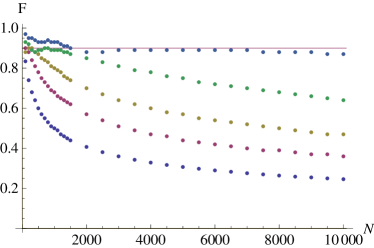
Figure 1: (Color online) Maximum fidelity which can be obtained as a function of $N$ for the states $\Psi_{2}$,$\Psi_{3}$, $\Psi_{4}$, $\Psi_{6}$, and $\Psi_{11}$. (From bottom to top. There are no crossings.) The horizontal line lies at 90$\%$.

IV Average Fidelity and the Magnetic Field

So far we have not mentioned the magnetic field contribution to the Hamiltonian (Eq. II.1). This is because the effect of such a field is to apply equal phase shifts to all initial encodings which lie in ${\cal{H}}^{(1)}$ and so the fidelities discussed thus far have been independent of $h$. We will now consider an encoded qubit which not only lies in ${\cal{H}}^{(1)}$ but in ${\cal{H}}^{(0)}$ as well. ${\cal{H}}^{(0)}$ and ${\cal{H}}^{(1)}$ are distinct eigenspaces of the operator of the total $z$ component of the spin; $\sigma_{tot}^{z}=\sum_{i=1}^{N}\sigma_{i}^{z}$. ${\cal{H}}^{(0)}$ is spanned by a single state, namely $\left|{\bf{0}}\right\rangle$, which is also an eigenstate of the total Hamiltonian $H$. The associated energy of the ground state is chosen to be zero and therefore the coefficient attached to $\left|{\bf{0}}\right\rangle$ in Eq. (III.3) will not change over time.

A global magnetic field is related to the fidelity through the transition amplitudes $f_{s,j}(t)$ in Eq. (II.4). For what follows let us re-express these amplitudes as $f_{s,j}(t)=e^{-2iht}\tilde{f}_{s,j}(t)$, where $\tilde{f}_{s,j}(t)=\frac{2}{N+1}\sum_{m=1}^{N}\sin{(q_{m}s)}\sin{(q_{m}j)}e^{2iJt\cos{(q_{m})}}$ is independent of $h$. The fidelity $F_{k}$ of state transfer for the encoding $\left|\xi_{k}\right\rangle$ can be calculated to be

$$F_{k} = \left[\cos^{4}{\frac{\theta}{2}}+\frac{1}{2k}\sin^{2}{\theta}\left(\text{Re}\left[e^{2iht}\sum_{m=1}^{k}(-1)^{m+1}C^{*}_{N+2(m-k)}(t)\right]+\sum_{m=1}^{N+1-2k}|C_{m}(t)|^{2}\right)\right.$$ (IV.1)

$$+ \left.\frac{1}{k^{2}}\sin^{4}{\frac{\theta}{2}}\left|\sum_{m=1}^{k}(-1)^{m+1}C^{*}_{N+2(m-k)}(t)\right|^{2}\right]^{1/2},$$

where $C_{\nu}(t)=\sum_{p=0}^{k-1}(-1)^{p}\tilde{f}_{2p+1,\nu}(t).$ Since the $C_{\nu}(t)$ are independent of the applied field $h$ the dependence of $F_{k}$ on this quantity comes strictly from the second term in Eq. (IV.1). If we let $L(t)=\frac{1}{k}\sum_{m=1}^{k}(-1)^{m+1}C^{*}_{N+2(m-k)}(t)$ we can express the second term of Eq. (IV.1) as

$$F_{h,k}=\frac{\sin^{2}{(\theta)}}{2}\left(\cos{(2ht)}\text{Re}\left[L(t)\right]-\sin{(2ht)}\text{Im}\left[L(t)\right]\right).$$ (IV.2)

It is shown in the appendix that $\tilde{f}_{s,j}(t)$ is purely real if $s$ and $j$ are both even or both odd and that $\tilde{f}_{s,j}(t)$ is purely imaginary if $s$ is even and $j$ is odd or $j$ is even and $s$ is odd. This implies that $L(t)$ is real when $N$ is odd and that $L(t)$ is imaginary when $N$ is even. In either case the fidelity will oscillate with respect to $h$ with a frequency given by $\nu=t/\pi.$ Since $\left|\Psi_{k}\right\rangle$ reaches its maximum fidelity at roughly $t_{0}\approx N/2$ (see Table I), the frequency of oscillation with $h$ is roughly $\nu\approx N/2\pi$ at the time at which $\left|\xi_{k}\right\rangle$ is to be measured. This increase in the sensitivity of $F_{k}$ to variations in $h$ as the chain grows larger can be seen in Fig. 2. There the solid and dashed lines respectively give the maximum fidelity for the states $(\left|{\bf{0}}\right\rangle+\left|\Psi_{2}\right\rangle)/\sqrt{2}$ and $(\left|{\bf{0}}\right\rangle+\left|\Psi_{4}\right\rangle)/\sqrt{2}$ as a function of $h$.

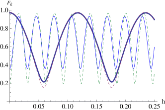
Figure 2: (Color online) Magnetic field dependence of the fidelity for the state $(\left|{\bf{0}}\right\rangle+\left|\Psi_{k}\right\rangle)/\sqrt{2}$. The solid (dashed) lines correspond to $k=2$ ($k=4$). The two lower (higher) frequency curves have been calculated for $N=51$ ($N=201$). Curves associated with a specific $k$ have been calculated with respect to the time which maximizes $\left|\Psi_{k}\right\rangle$.

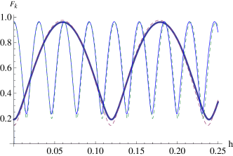
Figure 3: (Color online) Magnetic field dependence of the fidelity for the state $(\left|{\bf{0}}\right\rangle+\left|\Psi_{k}\right\rangle)/\sqrt{2}$. The solid (dashed) lines correspond to $k=3$ ($k=5$). The two lower (higher) frequency curves have been calculated for $N=51$ ($N=201$). Curves associated with a specific $k$ have been calculated with respect to the time which maximizes $\left|\Psi_{k}\right\rangle$.

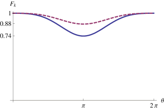
Figure 4: (Color online) Fidelity when transferring the state $\left|\xi_{k}\right\rangle$ over an isolated spin chain. The solid (dashed) line corresponds to $k=2,N=203$ ($k=3,N=201$). Curves associated with a specific $k$ have been calculated with respect to the time which maximizes $\left|\Psi_{k}\right\rangle$.

The graph clearly shows an increase in the frequency as the number of spins rises from $N=51$ to $N=201$. Also, since the fidelity of the state $\left|\Psi_{k}\right\rangle$ is given by $|L(t)|$ we see a decrease in the amplitude of these curves for increasing $N$. (Note that the square root results in an asymmetry of these curves about the value corresponding to $\cos{(2ht)}=0$.) The fact that the frequency grows linearly with $N$ suggests a technical challenge in the realization of these maximum fidelities for long chains. For example, for a chain composed of $N=10,000$ sites a change in $h$ on the order of $\Delta h\approx 10^{-4}$ will shift $F_{k}$ from its maximum value to its minimum value.

Instead of trying to maximize the value of $F_{k}$ by finely tuning some nonvanishing magnetic field, one could attempt to isolate the chain in order to achieve that same value if the number of sites are appropriately chosen. Since $L(t)$ is real when $N$ is an odd number the fidelity $F_{k}$ is either minimized or maximized when $h=0$ and $N$ is odd depending on whether $L(t)$ is positive or negative (see Eq. (IV.2)). For a given $k$ the sign of $L(t)$ alternates as the number of spins is increased by two. If $k$ is even the fidelity will be maximized (i.e, $L(t)$ is strictly positive) when $h=0$ if $N$ can be written as $N=3+4m$ for some integer $m$, otherwise $F_{k}$ will be minimized at $h=0$. Similarly, if $k$ is odd the fidelity will be maximized when $h=0$ if $N$ can be written as $N=1+4m^{\prime}$ for some other integer $m^{\prime}$, otherwise $F_{k}$ will be minimized at $h=0$

Figure 3 shows the magnetic field dependence of the fidelity for the states $(\left|{\bf{0}}\right\rangle+\left|\Psi_{3}\right\rangle)/\sqrt{2}$ and $(\left|{\bf{0}}\right\rangle+\left|\Psi_{5}\right\rangle)/\sqrt{2}$. The two higher frequency curves are nearly indistinguishable since the fidelities for $\left|\Psi_{3}\right\rangle$ and $\left|\Psi_{5}\right\rangle$, and thus the two amplitudes, are nearly equal for $N=201$ (see Table I).

When the applied field $h$ is chosen such that it maximizes $F_{k}$ the fidelity of the state $\left|\xi_{k}\right\rangle$ decreases smoothly from unity when $\theta=0$ to a minimum value when $\left|\xi_{k}\right\rangle=\left|\Psi_{k}\right\rangle$. (Notice that $F_{k}$ is independent of $\phi$.) This behavior is illustrated in Fig. 4 for $k=2$ and $k=3$. The fidelities shown in that figure have been calculated for isolated chains ($h=0$) containing $N=203$ and $N=201$ respective sites.

Since $\left|{\bf{0}}\right\rangle$ is an eigenstate of the Hamiltonian the average fidelity of $\left|\xi_{k}\right\rangle$ will be greater than the fidelity of $\left|\Psi_{k}\right\rangle$ alone when $h$ is chosen to maximize $F_{h,k}$. This occurs when $h$ takes on a value such that the product $\cos{(2ht)}{\mbox{Re}}[L(t)]$ or $\left(-\sin{(2ht)}{\mbox{Im}}[L(t)]\right)$ is positive and equal to $|L(t)|$. At these points the fidelity $F_{k}$ becomes

$$F_{k}^{max} = \left[\cos^{4}{\frac{\theta}{2}}+\frac{\sin^{2}{\theta}}{2}\left(|L(t)|+\frac{1}{k}\sum_{m=1}^{N+1-2k}|C_{m}(t)|^{2}\right)\right.$$ (IV.3)

$$+ \left.\sin^{4}{\frac{\theta}{2}}|L(t)|^{2}\right]^{1/2}.$$

The average fidelity of $F_{k}^{max}$ can be calculated as

$$F_{k}^{avg}=\frac{1}{2}\int\limits_{0}^{\pi}F_{k}^{max}\sin{(\theta)}d\theta$$ (IV.4)

Figure 5 exemplifies the high average fidelities which can be obtained when transferring the states $\left|\xi_{k}\right\rangle$ over long chains. Even for chains containing 10,000 sites the lowest value of the average fidelity, corresponding to $\left|\xi_{2}\right\rangle$, is still roughly $85\%$. For an $N=10,000$ spin chain the average fidelities associated with the states $\left|\xi_{3}\right\rangle$ and $\left|\xi_{11}\right\rangle$ are respectively $87\%$ and $96\%$.

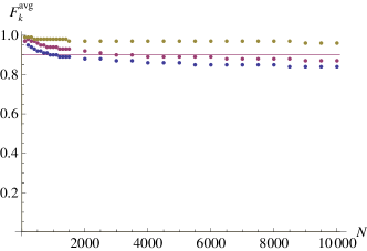
Figure 5: (Color online) Average fidelity of the states $\left|\xi_{k}\right\rangle$ for k=2,3, and 11. (From bottom to top. There are no crossings.) The horizontal line lies at 90$\%$.

V Optimal State Encoding

We will now compare our results to those which can be obtained using Haselgrove’s optimal encoding scheme H.L. Haselgrove (2005). Specifically, we will compare the maximum fidelities that can be obtained in either case for initial encodings that take place over equal regions of the chain.

In what follows we will assume that Alice and Bob respectively have access to the first and last $r$ sites of a linear spin chain and that the system evolves according to the Hamiltonian given by Eq. (II.1). Using the notation of T.J. Osborne and N. Linden (2004); H.L. Haselgrove (2005) we may express an arbitrary initial encoding of the chain as

$$\left|\Psi(0)\right\rangle=(\alpha\left|{\bf{0}}\right\rangle_{A}+\beta\left|1_{enc}\right\rangle_{A})\otimes\left|{\bf{0}}\right\rangle_{\bar{A}},$$ (V.1)

where $\left|1_{enc}\right\rangle_{A}\>\in\>\>{\cal{H}}^{(1)}$ and $A$ ($\bar{A}$) refers to the spins which Alice does (does not) control. Since $\left|{\bf{0}}\right\rangle$ is an eigenstate of the system we may write the evolved state $\left|\Psi(T)\right\rangle=e^{-iHT}\left|\Psi(0)\right\rangle$ in the general form

$$\left|\Psi(T)\right\rangle = \beta\sqrt{1-C_{B}(T)}\left|\eta(T)\right\rangle$$

$$+ \left|{\bf{0}}\right\rangle_{\bar{B}}[\alpha\left|{\bf{0}}\right\rangle_{B}+\beta\sqrt{C_{B}(T)}\left|\gamma(T)\right\rangle_{B}].$$

Here $C_{B}(T)$ gives the probability that the excitation has transferred into the receivers accessible region. $\left|\gamma(T)\right\rangle_{B}$ is a some normalized state that is orthogonal to $\left|{\bf{0}}\right\rangle_{B}$ and $\left|\eta(T)\right\rangle$ is some normalized state that is orthogonal to all states of the form $\left|{\bf{0}}\right\rangle_{\bar{B}}\otimes\left|\nu\right\rangle_{B}$. As was mentioned in the introduction, according to this protocol the receiver will apply a decoding unitary to his accessible spins such that the probability $C_{B}(T)$ will be transferred to a single spin site. After this has occurred the fidelity between the final output qubit state and the intended message state can be expressed as

$$\left[|\alpha|^{4}+[1+2\sqrt{C_{B}(T)}-C_{B}(T)]|\alpha|^{2}|\beta|^{2}+C_{B}(T)|\beta|^{4}\right]^{1/2}$$ (V.3)

(We note that the global square root does not appear in Ref. T.J. Osborne and N. Linden (2004).) Since we are only concerned with the $\left|1_{enc}\right\rangle_{A}$ states, we will set $\alpha=0$ and $\beta=1$. The fidelity associated with an encoding $\left|1_{enc}\right\rangle_{A}$ over the first $r$ spins of the chain is then

$$F_{r}=\sqrt{C_{B}(T)}.$$ (V.4)

If we let $P_{\cal{A}}$ and $P_{\cal{B}}$ represent the projectors onto Alice’s and Bob’s accessible subspaces we may express $C_{B}(T)$ as

$$C_{B}(T)=||P_{\cal{B}}\>e^{-iHt}\left|1_{enc}\right\rangle_{A}\otimes\left|{\bf{0}}\right\rangle_{\bar{A}}||^{2},$$ (V.5)

where $||\cdot||$ represents the $l_{2}$ norm. Haselgrove’s optimal states are those which maximize $C_{B}(T)$. They correspond to the first right singular vectors of $P_{\cal{B}}\>e^{-iHt}\>P_{\cal{A}}$. For an encoding which uses $r$ spins, we will refer to the optimal state as $\left|\Phi\right\rangle_{r}$.

Table 2 provides the maximum fidelities which can be obtained for the states $\left|\Phi\right\rangle_{r}$ ($r=3,5,7,9$) as a function of $N$. The difference between these maximum values and those associated with the states $\left|\Psi\right\rangle_{(r+1)/2}$ is given in terms of $\Delta_{r}$. We see that as the ratio of the number of encoded spins to the total number of spins approaches zero the value of $\Delta_{r}$ also goes to zero. The table also gives a measure of how close these states resemble the $\left|\Psi\right\rangle_{k}$ in terms of the quantity $d_{r}=|\left|\Phi\right\rangle_{r}-\left|\Psi\right\rangle_{(r+1)/2}|$. For large chains our states actually converge to the optimal states obtained using Haselgrove’s method. It is interesting to note that in all cases the times which maximize the fidelity is nearly the same for both our states and Haselgrove’s states for encodings that take place over the first $r$ spins. The fact that $\Delta_{r}$ approaches zero for large chains is also interesting since the fidelities which were calculated for our states were taken place before any decoding operation while the fidelities associated with Haselgrove’s states were determined after this assumed operation had occurred. This implies that for large chains the fidelities associated with these optimal states are independent of the decoding operation.

$\left|\Phi\right\rangle_{3}$

$N$		100		200		300		400		500		3000
$F_{3}$		.85		.75		.68		.64		.60		.36
$\Delta_{3}$		.02		.01		.00		.00		.00		.00
$d_{3}$		.13		.09		.07		.06		.05		.02
$t_{0}$		51.75		102.36		152.76		203.07		253.33		1506.14

$\left|\Phi\right\rangle_{5}$

$N$		100		200		300		400		500		3000
$F_{5}$		.96		.91		.86		.82		.79		.52
$\Delta_{5}$		.06		.03		.02		.01		.01		.01
$d_{5}$		.27		.19		.15		.13		.11		.04
$t_{0}$		51.08		101.74		152.20		202.55		252.84		1505.83

$\left|\Phi\right\rangle_{7}$

$N$		100		200		300		400		500		3000
$F_{7}$		.99		.97		.95		.92		.90		.64
$\Delta_{7}$		.11		.07		.05		.04		.03		.01
$d_{7}$		.40		.29		.25		.21		.19		.07
$t_{0}$		50.25		101.00		151.45		201.89		252.20		1505.51

$\left|\Phi\right\rangle_{9}$

$N$		100		200		300		400		500		3000
$F_{9}$		.99		.99		.98		.97		.96		.75
$\Delta_{9}$		.06		.11		.10		.07		.06		.01
$d_{9}$		.52		.40		.34		.29		.26		.12
$t_{0}$		49.4		100.21		150.74		201.14		251.49		1505.00

Table 2: Table showing the maximum fidelity achievable and the associated arrival times for the states $\left|\Phi_{r}\right\rangle$, $r=3,5,7,9$ as a function of $N$. $\Delta_{r}$ gives the difference between the maximum fidelities associated with $\left|\Phi_{r}\right\rangle$ and $\left|\Psi_{(}r+1)/2\right\rangle$. The quantity $d_{r}=|\left|\Phi\right\rangle_{r}-\left|\Psi\right\rangle_{(r+1)/2}|$ is also given. Note that the time has been calculated using $J=1.$

VI conclusion

The $k$-qubit encodings which we have introduced can be used to reliably transmit information over very large spin chains. Their simple structure was shown to yield high transfer fidelities after the system was allowed to evolve freely for some specified time. These successful transmissions did not require the dynamical control or individual design of the exchange couplings, nor did they require the implementation of decoding operations at the receiving end. When the chains are placed in a global magnetic field the fidelities associated with these states were found to become highly sensitive to fluctuations in the field strengths as the chains become large. The frequency of the fidelities oscillation with the field was determined to be proportional to the number of spins in the chain suggesting the technical difficulties associated with achieving these high values for large $N$. It was found that if the chain contained an appropriate number of sites the fidelity could be maximized when the chain was isolated from the field. When $k$ is an even number the fidelity will take its maximum value when $h=0$ if $N$ can be written as $N=3+4m$ for some integer $m$. Similarly, if $k$ is odd the fidelity will be maximized when $h=0$ if $N$ can be written as $N=1+4m^{\prime}$ for some other integer $m^{\prime}$.

A comparison with Haselgrove’s optimal encodings H.L. Haselgrove (2005) was also given. It was shown that for small chains his states will yield slightly higher fidelities than ours when the encodings are viewed to take place over the first $r$ spins of the chain. However, since our states only require the initialization of $k$ of the first $r=2k-1$ spins, preparation of our states would appear easier for near-future realization. For large chains our states converge to Haselgrove’s optimal encodings, and can transfer with fidelities that are independent of a decoding stage. It is interesting that these even site encodings yield much higher fidelities when compared to the analogous odd site encodings. However, the fundamental reason for their success in propagation remains unclear.

Given the simple structure inherent to our encodings, along with the minimal technical requirements needed for reliable transmission, we believe that these states could serve as useful message carriers over large spin chains.

VII Appendix

We will show here that the $\tilde{f}_{s,j}(t)=\frac{2}{N+1}\sum_{m=1}^{N}\sin{(q_{m}s)}\sin{(q_{m}j)}e^{2iJt\cos{(q_{m})}}$ are either purely real or purely imaginary. First notice that for $s=1,2,...,N$ and $\delta=0,1,2,...,N-1$ we have

$$\sin{(q_{(N-\delta)}s)} = \sin{(q_{s}(N-\delta))}$$

$$= \sin{(q_{s}N)}\cos{(q_{s}\delta)}-\cos{(q_{s}N)}\sin{(q_{s}\delta)},$$

with

$$\sin{(q_{s}N)}=(-1)^{s+1}\sin{(q_{s})}$$

and

$$\cos{(q_{s}N)}=(-1)^{s}\cos{(q_{s})}.$$

So we have the identity

$$\sin{(q_{(N-\delta)}s)}=(-1)^{s+1}\sin{(q_{(1+\delta)}s)}.$$ (VII.2)

It can also be shown that the following relation holds

$$\cos{(q_{(N-\delta)})}=-\cos{(q_{(1+\delta)})}.$$ (VII.3)

Equation (VII.2) implies that $\sin{(q_{(1+\delta)}s)}\sin{(q_{(1+\delta)}j)}=\sin{(q_{(N-\delta)}s)}\sin{(q_{(N-\delta)}j)}$ if $s$ and $j$ are both even or both odd, and that $\sin{(q_{(1+\delta)}s)}\sin{(q_{(1+\delta)}j)}=-\sin{(q_{(N-\delta)}s)}\sin{(q_{(N-\delta)}j)}$ if $s$ or $j$ is even while the other is odd. Let us now consider four cases.

Case (1): The number of spins $N$ is even while $s$ and $j$ are both even or both odd. In this case the $(1+\delta)th$ term of the series $\text{Re}\left[\tilde{f}_{s,j}(t)\right]=\frac{2}{N+1}\sum_{m=1}^{N}\sin{(q_{m}s)}\sin{(q_{m}j)}\cos{(2Jt\cos{(q_{m})})}$ will equal the $(N-\delta)th$ term since $\cos{(-x)}=\cos{(x)}$. Also, since $N$ is even every term in the series can be matched with another term. Since $\sin{(x)}=-\sin{(-x)}$ the $(1+\delta)th$ term of the series $\text{Im}\left[\tilde{f}_{s,j}(t)\right]=\frac{2}{N+1}\sum_{m=1}^{N}\sin{(q_{m}s)}\sin{(q_{m}j)}\sin{(2Jt\cos{(q_{m})})}$ will cancel with the $(N-\delta)th$ term. $N$ is even so every term will cancel. In this case $\tilde{f}_{s,j}(t)=\text{Re}\left[\tilde{f}_{s,j}(t)\right]$.

Case (2): The number of spins $N$ is odd while $s$ and $j$ are both even or both odd. The situation here is the same as for the previous case except now one has to account for the $(N+1)/2\>th$ term. Since $\cos{(2Jt\cos{(q_{(N+1)/2})})}=1$ and $\sin{(2Jt\cos{(q_{(N+1)/2})})}=0$ we find that $\text{Im}\left[\tilde{f}_{s,j}(t)\right]=0$ again for this second case. Consequently $\tilde{f}_{s,j}(t)=\text{Re}\left[\tilde{f}_{s,j}(t)\right]$.

Case (3): $N$ and $s$ are even while $j$ is odd or $N$ and $j$ are even while $s$ is odd. In this case the $(1+\delta)th$ term will equal (cancel) the $(N-\delta)th$ term of the series expansion for $\text{Im}\left[\tilde{f}_{s,j}(t)\right]$ ($\text{Re}\left[\tilde{f}_{s,j}(t)\right]$). $N$ is assumed to be even here so every term in $\text{Re}\left[\tilde{f}_{s,j}(t)\right]$ will cancel with another term. In this case $\tilde{f}_{s,j}(t)=\text{Im}\left[\tilde{f}_{s,j}(t)\right]$.

Case (4): $N$ and $s$ are odd while $j$ is even or $N$ and $j$ are odd while $s$ is even. Again, the only difference between this case and the last is due to the fact that the $(N+1)/2\>th$ term cannot be matched up with another term. This middle term is zero for $\text{Im}\left[\tilde{f}_{s,j}(t)\right]$ as it was in case two. For $\text{Re}\left[\tilde{f}_{s,j}(t)\right]$ this term is equal to $\frac{2}{N+1}\sin{(\pi s/2)}\sin{(\pi j/2)}=0$ since either $s$ or $j$ is even. So for this case $\tilde{f}_{s,j}(t)=\text{Im}\left[\tilde{f}_{s,j}(t)\right]$.

In every case $\tilde{f}_{s,j}(t)$ is either purely real or purely imaginary. Whether $\tilde{f}_{s,j}(t)$ is real or imaginary depends on the indices $s$ and $j$. Regardless of the number of spins in the chain, $\tilde{f}_{s,j}(t)$ is real if $s$ and $j$ are both even or both odd and $\tilde{f}_{s,j}(t)$ is imaginary if $s$ is even and $j$ is odd or $j$ is even and $s$ is odd.

References

- S. Bose (2003) S. Bose, Phys. Rev. Lett. 91, 207901 (2003).
- L.-A. Wu, Y. Liu, F. Nori (2009) L.-A. Wu, Y. Liu, F. Nori (2009), arXiv:quant-ph/0903.2154.
- G. M. Nikolopoulos, D. Petrosyan and P. Lambropoulos (2004) G. M. Nikolopoulos, D. Petrosyan and P. Lambropoulos, Europhys. Lett. 65, 297 (2004).
- G.M. Nikolopoulos, D. Petrosyan, P. Lambropoulos (2004) G.M. Nikolopoulos, D. Petrosyan, P. Lambropoulos, J. Phys: Cond. Mat. 16, 4991 (2004).
- M. Christandl, N. Datta, A. Ekert, and A.J. Landahl (2004) M. Christandl, N. Datta, A. Ekert, and A.J. Landahl, Phys. Rev. Lett. 92, 187902 (2004).
- M. Christandl, N. Datta, T.C. Dorlas, A. Ekert, A. Kay, and A.J. Landahl (2005) M. Christandl, N. Datta, T.C. Dorlas, A. Ekert, A. Kay, and A.J. Landahl, Phys. Rev. A 71, 032312 (2005).
- H.L. Haselgrove (2005) H.L. Haselgrove, Phys. Rev. A 72, 062326 (2005).
- D. Burgarth, V. Giovannetti, and S. Bose (2007) D. Burgarth, V. Giovannetti, and S. Bose, Phys. Rev. A 75, 062327 (2007).
- C. Di Franco, M. Paternostro, and M.S.Kim (2008) C. Di Franco, M. Paternostro, and M.S.Kim, Phys. Rev. Lett. 101, 230502 (2008).
- T.J. Osborne and N. Linden (2004) T.J. Osborne and N. Linden, Phys. Rev. A 69, 052315 (2004).
- J. Allcock and N. Linden (2009) J. Allcock and N. Linden, Phys. Rev. Lett. 102, 110501 (2009).
- Wang et al. (2009) Z.-M. Wang, C. A. Bishop, M. S. Byrd, B. Shao, and J. Zou, Phys. Rev. A 80, 022330 (2009).
- S. Bose (2007) S. Bose, Contemp. Phys. 48, 13 (2007).
- M. Hase, H. Kuroe, K. Ozawa, O. Suzuki, H. Kitazawa, G. Kido, and T. Sekine (2004) M. Hase, H. Kuroe, K. Ozawa, O. Suzuki, H. Kitazawa, G. Kido, and T. Sekine, Phys. Rev. B 70, 104426 (2004).