Abstract

The effective separable meson-baryon potentials are constructed to match the equivalent chiral amplitudes up to the second order in external meson momenta. We fit the model parameters (low energy constants) to the threshold and low energy $K^{-}p$ data. In the process, the $K^{-}$-proton bound state problem is solved exactly in the momentum space and the 1s level characteristics of the kaonic hydrogen are computed simultaneously with the available low energy $K^{-}p$ cross sections. The model is also used to describe the $\pi\Sigma$ mass spectrum and the energy dependence of the $K^{-}n$ amplitude.

PACS: 11.80.Gw, 12.39.Fe, 13.75.Jz, 36.10.Gv
Keywords: chiral Lagrangians, coupled channels, kaonic atoms

1 Introduction

The meson-baryon interactions at low energies have become a testing ground for theoretical models based on chiral symmetry. Since the pioneering works of Weinberg [1], Gasser, Leutwyler [2] and others (see [3] for a comprehensive overview) the chiral perturbation theory has been established as the effective field theory of strong interactions that implements the QCD symmetries in a region where perturbative QCD is inapplicable. In the SU(2) sector the ChPT proved to be quite successful thanks to very small current masses of the $u$ and $d$ quarks. The smallness of the pion mass also complies well with its presumed origin as that of the Goldstone boson.

The situation becomes more intriguing once we enter the strange sector. Especially, the treatment of the kaon-nucleon interaction at low energies requires a special care. Unlike the pion-nucleon interaction the $\bar{K}N$ dynamics is strongly influenced by the existence of the $\Lambda(1405)$ resonance, just below the $K^{-}p$ threshold. This means that the standard chiral perturbation series do not converge. Fortunately, one can use non-perturbative coupled channel techniques to deal with the problem and generate the $\Lambda(1405)$ resonance dynamically. Though such approach violates the crossing symmetry it has proven quite useful and several authors have already applied it to various low energy meson-baryon processes [4]-[9].

While the properties of the $\Lambda(1405)$ resonance have been well known for a long time, the nature of the resonance still remains a mystery. For many years it has been considered as a meson-baryon quasi-bound state coupled to the $\pi\Sigma$ and $\bar{K}N$ channels [10]. It can also be viewed as a standard $qqq$ baryon [11] and some authors have advocated the notion that the resonance is a pentaquark state [12]. Recently, it was also realized that the chiral models generate two poles in the complex energy plane that can be assigned to the $\Lambda(1405)$ [13], [14]. Although the ”two poles model” may look viable and supported by the analysis [15] of the $K^{-}p\rightarrow\pi^{0}\pi^{0}\Sigma^{0}$ measurement [16] it is still not quite clear if (and how) this particular set of experimental data is compatible with the results of other experiments related to the lineshape of the $\Lambda(1405)$ resonance. We will come back to this point in Section 4.2 while discussing the relevant pole structure and the $\pi\Sigma$ mass spectrum generated by our model.

There is a plenty of experimental data on various processes initiated by the $K^{-}p$ interaction at low energies. The relatively old data on cross sections and threshold branching ratios were supplemented by recent measurements of strong interaction effects on the 1s level of kaonic hydrogen (KEK [17] and DEAR collaboration in Frascati [18]). Although the measurements have confirmed the repulsive character of the $K^{-}p$ strong interaction at threshold the DEAR values of the strong interaction shift and width of the 1s level look at odds with the $K^{-}p$ scattering length extrapolated from the scattering measurements. In this report we present our analysis of the situation and discuss the compatibility of the kaonic hydrogen measurement with other data. The novelty of our approach lies in exact calculation of the $K^{-}p$ bound state properties instead of relying on the approximate Deser-Trueman relation [19] (or its version modified to include the isospin effects and electromagnetic corrections [20]). Our separable potential model can also serve as a viable alternative to the N/D scheme based on a dispersion relation for the inverse of the T-matrix that employs techniques and language common in high energy physics. The separable potentials are well suited for any few body calculations that involve the $\bar{K}N$ interactions at low energies. Particularly, it should not be difficult to adapt our model for the Faddeev type calculations of the $\bar{K}NN-\pi\Sigma N$ system [21].

A brief account of our work was already given in [22]. Here we expand the letter not only by providing more details on our approach but include also a discussion of the $\Lambda(1405)$ resonance spectrum and present our results for the $K^{-}n$ scattering amplitude. Since the scope of the article is wider than in our previous work and we apply our model to a broader interval of the $\bar{K}N$ energies (specifically below the $\bar{K}N$ threshold) we put additional constraints on the model parameters and present completely new fits to the data with those constraints in effect.

Our main aim remains a simultaneous description of both the 1s level kaonic bound state and the available experimental data for the $K^{-}p$ initiated processes. The characteristics of kaonic hydrogen 1s level are computed precisely with the same effective chiral potentials that are used to calculate the properties of $K^{-}p$ induced reactions. As we showed in [22], the direct computation of the kaonic hydrogen characteristics is becoming necessary in view of the experimental precision expected in the SIDDHARTA measurement executed in Frascati [23]. At the same time our results for the $K^{-}n$ elastic amplitude are relevant to the measurement of kaonic deuterium performed by the same collaboration.

The article is organized as follows. First we outline the method we use to calculate the quantities observed in low energy $K^{-}p$ interactions, then we present the chiral Lagrangian used to derive our effective meson-baryon potentials. Main part of the paper is given in Section 4 where we present and discuss the results obtained in our fits to the $K^{-}p$ experimental data and proceed with the analysis of the $\pi\Sigma$ mass spectrum and the $K^{-}n$ interactions. Our conclusions are briefly summarized in the last section.

2 Method outlined

We developed a precise method of computing the meson-nuclear bound states in momentum space. The method was already applied to pionic atoms [24] and its multichannel version was used to calculate the 1s level characteristics of pionic hydrogen [25]. Here we just remark that our approach is based on the construction of the Jost matrix and involves the solution of the Lippman-Schwinger equation for the transition amplitudes between various channels. Bound states in a specific channel then correspond to zeros of the determinant of the Jost matrix at (or close to) the positive part of the imaginary axis in the complex momentum plane. The zeros are searched for iteratively by means of the Mueller algorithm. If only the point-like Coulomb potential is considered in the $K^{-}p$ channel the method reproduces the well known Bohr energy of the 1s level with a precision better than $0.1$ eV. The inclusion of the leading electromagnetic corrections, the charge finite sizes and vacuum polarization effects, gives an attractive energy shift $\Delta E_{FS+VP}(1s)=-20.2$ eV.

The necessary ingredient needed to calculate the impact of strong interaction on $K$-atomic energy levels is the kaon-nuclear optical potential. In the case of kaonic hydrogen and multiple channels it means the potential matrix. We follow the approach of Ref. [4] and construct the strong interaction part of the potential matrix as effective transition amplitudes that give the same (up to the order $\mathcal{O}(q^{2})$ of the external meson momenta) s-wave scattering lengths as are those derived from the underlying chiral Lagrangian. While the authors of Ref. [4] restricted themselves only to the first six meson-baryon channels that are open at the $\bar{K}N$ threshold we employ all ten coupled meson-baryon channels: $\pi^{0}\Lambda$, $\pi^{0}\Sigma^{0}$, $\pi^{-}\Sigma^{+}$, $\pi^{+}\Sigma^{-}$, $K^{-}p$, $\bar{K}^{0}n$, $\eta\Lambda$, $\eta\Sigma^{0}$, $K^{0}\Xi^{0}$, and $K^{+}\Xi^{-}$. We order the channels according to their threshold energies and will refer to them (and index them) in this particular order. As we already mentioned in the Introduction the $\Lambda(1405)$ resonance does not enter as a separate field but it is generated dynamically by solving coupled Lippman-Schwinger equations with the input potential matrix.

The strong interaction potential matrix is given in the separable form

$$V_{ij}(k,k^{\prime})=\sqrt{\frac{1}{2E_{i}}\frac{M_{i}}{\omega_{i}}}\>g_{i}(k)\>\frac{C_{ij}}{f^{2}}\>g_{j}(k^{\prime})\>\sqrt{\frac{1}{2E_{j}}\frac{M_{j}}{\omega_{j}}},\quad g_{j}(k)=\frac{1}{1+(k/\alpha_{j})^{2}}$$ (1)

in which the momenta $k$ and $k^{\prime}$ refer to the meson-baryon c.m. system in the $i$ and $j$ channels, respectively. The kinematical factors $\sqrt{M_{j}/(2E_{j}\omega_{j})}$ guarantee a proper relativistic flux normalization with the meson energy $E_{j}$ and the baryon mass and energy $M_{j}$ and $\omega_{j}$, all taken in the c.m. system of channel $j$. The off shell form factors $g_{j}(k)$ introduce the inverse range radii $\alpha_{j}$ that characterize the radius of interactions in various channels. Finally, the parameter $f\simeq 100$ MeV (a value between the empirical pion and kaon decay constants) stands for the pseudoscalar meson decay constant in the chiral limit and the coupling matrix $C_{ij}$ is determined by chiral SU(3) symmetry and includes terms up to the second order in the meson c.m. kinetic energies. The details on the underlying chiral Lagrangian and on the couplings $C_{ij}$ will be given in the following section.

The potential of Eq. (1) is used not only when solving the bound state problem but we also implement it in the standard Lippman-Schwinger equation and compute the low energy $\bar{K}N$ cross sections and branching ratios from the resulting transition amplitudes. Our LS equation for the s-wave coupled channel T-matrix and the separable potential (1) can be written in a purely algebraic form,

$$t_{ij}=v_{ij}+\displaystyle\sum_{n}v_{in}\>I_{n}\>t_{nj}\;\;\;,$$ (2)

where we introduced the notation $T_{ij}=t_{ij}g_{i}g_{j}$ and $V_{ij}=v_{ij}g_{i}g_{j}$ (the obvious dependence on kinematical variables is not shown here for simplicity). In vacuum, the integral $I_{n}$ can be evaluated analytically,

$$I_{n}=2\mu_{n}\int\frac{d^{3}l}{(2\pi)^{3}}\>\frac{g^{2}_{n}(l)}{k^{2}_{n}-l^{2}+i\epsilon}=-\frac{\mu_{n}}{2\pi}\>\frac{(\alpha_{n}+ik_{n})^{2}}{2\alpha_{n}}\>g^{2}_{n}(k_{n})\;\;\;.$$ (3)

Here $k_{n}$ stands for the on-shell meson-baryon relative momenta in the intermediate channel $n$ and $\mu_{n}$ denotes the ”reduced mass” of the system, $\mu_{n}=E_{n}\omega_{n}/(E_{n}+\omega_{n})$. The nonrelativistic scattering amplitude $f_{ij}$ for the transition from channel $j$ to channel $i$ is then simply obtained by solving the system of algebraic equations (2) and by using the relation $f_{ij}=-\sqrt{\mu_{i}\mu_{j}}\,T_{ij}/(2\pi)$. The observable quantity, the total s-wave cross section for the transition, is given by the standard formula,

$$\sigma_{ij}=4\pi\>\frac{k_{i}}{k_{j}}\>|f_{ij}|^{2}\;\;\;.$$ (4)

The reader should note that our approach differs from the recently more popular on-shell N/D scheme based on the Bethe-Salpeter equation, unitarity relation for the inverse of the $T$-matrix and on the dimensional regularization of the scalar loop integral [13]. Though the difference is only a technical one it has consequences. The advantage of our method is that the off-shell form factors are parameterized by means of the inverse range radii which have a better physical meaning than the subtraction constants appearing due to the regularization procedure used in the inverse $T$-matrix approach . In principle the off-shell effects can be incorporated in the latter model too. However, in our approach they appear quite naturally with no additional effort. On the other hand the use of Bethe-Salpeter equation and quantum field techniques makes the other model more attractive it terms of completely relativistic dynamics while we restrict ourselves only to relativistic treatment of the kinematical variables. This restriction is fully justified in the region of low and intermediate energies that are the subject of our work.

3 Chiral Lagrangian

In this section we briefly outline the effective chiral Lagrangian that is based on the $SU(3)_{\rm L}\otimes SU(3)_{\rm R}$ chiral symmetry and reflects the symmetries of QCD. It describes the coupling of the pseudoscalar meson octet ($\pi$, $K$, $\bar{K}$, $\eta$) to the ground state baryon octet ($N$, $\Lambda$, $\Sigma$, $\Xi$). Following Ref. [4] we consider the first two orders (in terms of the external meson momenta and quark masses) of the Lagrangian density,

$${\cal L}={\cal L}^{(1)}+{\cal L}^{(2)}.$$ (5)

The leading order reads

$${\cal L}^{(1)}=Tr(\overline{\Psi}_{B}(i\gamma_{\mu}D^{\mu}-M_{0})\Psi_{B})+F\,Tr(\overline{\Psi}_{B}\gamma_{\mu}\gamma_{5}[u^{\mu},\Psi_{B}])+D\,Tr(\overline{\Psi}_{B}\gamma_{\mu}\gamma_{5}\{u^{\mu},\Psi_{B}\})$$ (6)

where the covariant derivative is given by

$$D^{\mu}\Psi_{B}=\partial^{\mu}\Psi_{B}+[{1\over{8f^{2}}}[\phi,\partial^{\mu}\phi],\Psi_{B}]+\dots$$ (7)

and the axial matrix operator is

$$u^{\mu}=-\frac{1}{2f}\partial^{\mu}\phi+\dots\;.$$ (8)

The meson and (heavy) baryon fields are represented by the matrices $\phi$ and $\Psi_{B}$, respectively. Further, $M_{0}$ is the baryon mass in the chiral limit and the constants $F$ and $D$ are the $SU(3)$ axial vector couplings.

The leading order (linear in the external meson four-momentum $q$) of Eq. (6) is the current algebra, or the Weinberg-Tomozawa, term. In addition, the Lagrangian ${\cal L}^{(1)}$ gives rise to s-wave meson-baryon amplitudes at order $q^{2}$ (and higher). They appear due to relativistic corrections to the covariant derivative term and due to the Born graphs terms that originate from the axial coupling part of ${\cal L}^{(1)}$. These $q^{2}$ pieces add to the relevant s-wave terms of the second order Lagrangian,

$${\cal L}^{(2)} = b_{D}Tr(\overline{B}\{\chi_{+},B\})+b_{F}Tr(\overline{B}[\chi_{+},B])+b_{0}Tr(\overline{B}B)Tr(\chi_{+})$$

$$+ d_{D}Tr(\overline{B}\{(u^{2}+(v\cdot u)^{2}),B\})+d_{F}Tr(\overline{B}[(u^{2}+(v\cdot u)^{2}),B])$$

$$+ d_{0}Tr(\overline{B}B)Tr(u^{2}+(v\cdot u)^{2})$$

$$+ d_{1}(Tr(\overline{B}u_{\mu})Tr(u^{\mu}B)+Tr(\overline{B}(v\cdot u))Tr((v\cdot u)B))$$

$$+ d_{2}Tr(\overline{B}(u_{\mu}Bu^{\mu}+(v\cdot u)B(v\cdot u)))+\cdots$$

which, at the tree level, also generates contributions of the order $q^{2}$. We have denoted

$$\chi_{+}=-{1\over{4f^{2}}}\{\phi,\{\phi,\chi\}\}$$ (10)

and $v^{\mu}$ is the baryon four-velocity, $v^{\mu}=(1,0,0,0)$ for baryon at rest. The $\chi$ matrix introduces explicit chiral symmetry breaking and is proportional to the quark mass matrix with only diagonal elements not equal to zero. In the isospin symmetry limit, the diagonal elements are $(m^{2}_{\pi},m^{2}_{\pi},2m^{2}_{K}-m^{2}_{\pi})$.

Figure 1: The Feynman diagrams relevant for the s-wave meson-baryon interaction.

$\mathcal{O}(q^{1})$ contact	$\mathcal{O}(q^{2})$ contact	direct s-term	crossed u-term

When the effective meson-baryon potentials (1) are constructed to match the Born amplitudes generated by the chiral Lagrangian the low energy constants (the couplings at various terms in the Lagrangian) combine to the couplings $C_{ij}$ that bind the considered meson-baryon states. Thus, the chiral symmetry of meson-baryon interactions is reflected in the structure of the $C_{ij}$ coefficients derived directly from the Lagrangian. The general structure of the couplings reads as

$$C_{ij} = -C_{ij}^{\rm(WT)}\,\frac{\>\!E^{\prime}_{i}+E^{\prime}_{j}\!\>}{4}\>+\>C_{ij}^{(mm)}\>\!\left(m_{i}^{2}+m_{j}^{2}\right)\>+\>C_{ij}^{(\chi{\rm b})}\>\!\left(m_{K}^{2}-m_{\pi}^{2}\right)+\>C_{ij}^{(EE)}\,E_{i}^{\rule{0.0pt}{3.01389pt}}E_{j}^{\rule{0.0pt}{3.01389pt}}+$$

$$\rule{0.0pt}{4.30554pt}\>+\>C_{ij}^{(s)}\,\frac{\>\!E_{i}^{\rule{0.0pt}{3.01389pt}}E_{j}^{\rule{0.0pt}{3.01389pt}}}{2M_{0}^{\rule{0.0pt}{3.01389pt}}\!\>}\>\rule{0.0pt}{4.30554pt}+\>C_{ij}^{(u)}\,\frac{1}{\>\!3M_{0}^{\rule{0.0pt}{3.01389pt}}\!\>}\,\left(2m_{i}^{2}+2m_{j}^{2}+\frac{\>\!m_{i}^{2}m_{j}^{2}\!\>}{E_{i}^{\rule{0.0pt}{3.01389pt}}E_{j}^{\rule{0.0pt}{3.01389pt}}}-\textstyle{\frac{7}{2}}E_{i}^{\rule{0.0pt}{3.01389pt}}E_{j}^{\rule{0.0pt}{3.01389pt}}\right)\;,$$ (11)

where the primed meson energies $E^{\prime}_{j}$ include the relativistic correction, $E^{\prime}_{j}=E_{j}+(E_{j}^{2}-m^{2}_{j})/(2M_{0})$, with $m_{j}$ denoting the meson mass in the channel $j$. The terms marked by the superscripts ”WT”, ”s” and ”u” correspond to the leading Weinberg-Tomozawa contact interaction and to the direct and crossed Born amplitudes, respectively. The remaining parts contribute to the contact interaction in the next-to-leading (i.e. $q^{2}$) order. For brevity we show the pertinent graphs in Figure 1 which we take from Ref. [8]. The terms $(mm)$ and $(\chi{\rm b})$ both appear due to explicit breaking of the chiral symmetry. In fact, what we denoted as the $(\chi{\rm b})$ term represents even the violation of the vector $SU(3)_{V}$ symmetry that is reduced to the isospin $SU(2)_{V}$ symmetry, i.e. the flavor symmetry of the $SU(3)$ octets is broken by this term.

The actual composition of the coefficients $C_{ij}^{\rm(.)}$ is given in the Appendices. We note that the coefficients for the first six channels coupled to the $K^{-}p$ system that are open at the $\bar{K}N$ threshold were already published in [4] while in Appendix A we show the complete tables for all ten considered channels. The couplings $C_{ij}$ can be related to their counterparts used in the alternative approach based on the chiral Lagrangian that is manifestly invariant to Lorentz transformations. The relation was derived in Ref. [26] for the case of the $SU(2)$ chiral symmetry. The derivation for the $SU(3)$ case is more complex and goes beyond the scope of the present work. In principle, the approaches based on both formulations of the chiral Lagrangian should give the same results for physical observables. However, this is true only when one sums up all orders of the infinite series of the relevant Feynman diagrams (all orders in $q$), not once we restrict ourselves to a given perturbative order (here $q^{2}$). This means that our results provided in the next section may (to a reasonable extent) differ from those achieved with the alternative formulation of the Lagrangian.

4 Results

In this section we closely follow the line presented in our letter [22] and show the results of our fits to the available low energy $\bar{K}N$ experimental data. While in [22] we aimed our analysis only at the kaonic hydrogen characteristics, the $K^{-}p$ threshold branching ratios and at the cross sections of $K^{-}p$ initiated reactions, here we also include the position of the $\Lambda(1405)$ resonance observed in the $\pi\Sigma$ mass spectrum. Additionally, we also present an analysis of the $K^{-}n$ scattering amplitude and discuss the effects due to breaking of isospin symmetry.

4.1 $\bar{K}N$ data fits

The three precisely measured threshold branching ratios [27] are

$$\gamma = \frac{\sigma(K^{-}p\rightarrow\pi^{+}\Sigma^{-})}{\sigma(K^{-}p\rightarrow\pi^{-}\Sigma^{+})}=2.36\pm 0.04~{},$$

$$R_{c} = \frac{\sigma(K^{-}p\rightarrow\hbox{charged particles})}{\sigma(K^{-}p\rightarrow\hbox{all})}=0.664\pm 0.011~{},$$ (12)

$$R_{n} = \frac{\sigma(K^{-}p\rightarrow\pi^{0}\Lambda)}{\sigma(K^{-}p\rightarrow\hbox{all neutral states})}=0.189\pm 0.015~{}.$$

They impose quite tight constraints on any model applied to the $\bar{K}N$ interactions at low energies.

The cross sections of $K^{-}p$ initiated reactions are not determined so accurately, thus they do not restrict the fits so much. We consider only the experimental data taken at the kaon laboratory momenta $p_{LAB}=110$ MeV (for the $K^{-}p$, $\bar{K^{0}}n$, $\pi^{+}\Sigma^{-}$, $\pi^{-}\Sigma^{+}$ final states) and at $p_{LAB}=200$ MeV (for the same four channels plus $\pi^{0}\Lambda$ and $\pi^{0}\Sigma^{0}$). Although some authors include in their fits the experimental cross sections at all available kaon momenta we feel that such approach unduely magnifies the importance of this particular set of data at expense of all other measurements that are not represented by so many data points. Anyway, our results show that the inclusion of the cross section data taken at many kaon momenta is not necessary since the fit at just $1-2$ points fixes the cross section magnitude and the energy dependence is reproduced nicely by the model.

We apply the same philosophy to the measured $\pi\Sigma$ mass distribution and fit only the position of the peak at 1395 MeV instead of fitting the complete measured spectra. Again, this appears to be quite sufficient as we will see in Section 4.2. In a manner of Ref. [13] we assume that the $\pi\Sigma$ mass distribution originates from a generic $s$-wave isoscalar source which couples to the $\bar{K}N$ and $\pi\Sigma$ $I=0$ states. Since the measured event distribution is not normalized, only the ratio of the relevant couplings $r=r_{\bar{K}N}/r_{\pi\Sigma}$ is of significance. In other words, we assume that the observed $\pi\Sigma$ spectrum complies with the prescription

$$dN_{\pi\Sigma}/dE\sim\bigg{|}T_{\pi\Sigma,\pi\Sigma}(I=0)+r_{KN/\pi\Sigma}\>T_{\pi\Sigma,\bar{K}N}(I=0)\bigg{|}^{2}p_{\pi\Sigma}$$ (13)

where the ratio $r_{KN/\pi\Sigma}$ is energy independent. In general, the ratio should be a complex number but (to further simplify the matter) we consider only real values in our fits. Though the reality may not be so simple the ansatz looks appropriate for simulating the dynamics of the $\Lambda(1405)$ resonance.

Finally, we include the DEAR results [18] on the strong interaction shift $\Delta E_{N}$ and the width $\Gamma$ of the 1s level in kaonic hydrogen:

$$\Delta E_{N}(1s)=(193\pm 43)\hbox{ eV,}\;\;\;\Gamma(1s)=(249\pm 150)\hbox{ eV~{}.}$$ (14)

Thus, we end up with a total of 16 data points in our fits.

The parameters of our model are: a) the couplings of the chiral Lagrangian which enter the coefficients $C_{ij}$, b) the inverse range radii $\alpha_{j}$ that provide the off-shell behavior of the potentials $V_{ij}$ of Eq. (1), c) the ratio $r_{KN/\pi\Sigma}$ determining the relative coupling of the $\bar{K}N$ and $\pi\Sigma$ channels to the $\Lambda(1405)$ resonance. Apparently, the number of parameters is too large, so it is desirable to fix some of them prior to performing the fits. First, the axial couplings $D$ and $F$ were already established in the analysis of semileptonic hyperon decays [28], $D=0.80$, $F=0.46$ ($g_{A}=F+D=1.26$). Then, we set the couplings $b_{D}$ and $b_{F}$ to satisfy the approximate Gell-Mann formulas for the baryon mass splittings,

$$M_{\Xi}-M_{N} = -8b_{F}(m_{K}^{2}-m_{\pi}^{2})$$

$$M_{\Sigma}-M_{\Lambda} = \frac{16}{3}b_{D}(m_{K}^{2}-m_{\pi}^{2})~{},$$ (15)

which gives $b_{D}=0.064$ GeV^-1 and $b_{F}=-0.209$ GeV^-1. Similarly, we determine the coupling $b_{0}$ and the baryon chiral mass $M_{0}$ from the relations for the pion-nucleon sigma term $\sigma_{\pi N}$ and the proton mass,

$$\sigma_{\pi N} = -2m_{\pi}^{2}(2b_{0}+b_{D}+b_{F})~{},$$

$$M_{p} = M_{0}-4m_{K}^{2}(b_{0}+b_{D}-b_{F})-2m_{\pi}^{2}(b_{0}+2b_{F})~{}.$$ (16)

Since the value of the pion-nucleon $\sigma$-term is not well established we enforce four different options, $\sigma_{\pi N}=$ (20–50) MeV, which cover the interval of the values considered by various authors. Finally, we reduce the number of the inverse ranges $\alpha_{j}$ to only five: $\alpha_{KN}$, $\alpha_{\pi\Lambda}$, $\alpha_{\pi\Sigma}$, $\alpha_{\eta\Lambda/\Sigma}$, $\alpha_{K\Xi}$. This leaves us with 12 free parameters: the five inverse ranges, the meson-baryon chiral coupling $f$, the ratio $r_{KN/\pi\Sigma}$ of Eq. (13) and five more low energy constants from the second order chiral Lagrangian denoted by $d_{D}$, $d_{F}$, $d_{0}$, $d_{1}$, and $d_{2}$.

The number of the second order couplings can be reduced even further since the pertinent Lagrangian terms are not completely independent. Thanks to the Cayley-Hamilton identity any of the Lorentz invariants contributing to the second order Lagrangian (3) with the $d$-couplings can be expressed as a linear combination of the other four invariants. This feature is reflected in the SU(3) chiral coefficients $C_{ij}$ which are invariant under the transformation

$$\begin{array}[]{lcccl}d_{D}&\longrightarrow&d_{D}^{\prime}&=&d_{D}+\Delta\\ d_{F}&\longrightarrow&d_{F}^{\prime}&=&d_{F}\\ d_{0}&\longrightarrow&d_{0}^{\prime}&=&d_{0}-\Delta/2\\ d_{1}&\longrightarrow&d_{1}^{\prime}&=&d_{1}-\Delta\\ d_{2}&\longrightarrow&d_{2}^{\prime}&=&d_{2}+\Delta\end{array}$$ (17)

for any real $\Delta$. In other words, one of the couplings (besides $d_{F}$) can be set to zero. While in our previous work we did not use this property here we set $d_{2}=0$ and fit only the remaining low energy constants.

Our results are summarized in Tables 1 - 3. The first table shows the results of our $\chi^{2}$ fits compared with the relevant experimental data. The resulting $\chi^{2}$ per data point indicate satisfactory fits. It is worth noting that their quality and the computed values do not depend much on the exact value of the $\sigma_{\pi N}$ term. Tables 2 and 3 show the fitted parameters of the chiral Lagrangian and the inverse range parameters $\alpha_{j}$. The last rows in the tables compare our values with those determined in Ref. [4] (with the $d$-couplings shifted according to Eq. (17) to satisfy the condition $d_{2}=0$). The reader may note that the fitted parameters differ significantly from those given in our earlier report [22]. The main reason for this is that in the present fits we decided to restrict the values of the inverse ranges $\alpha_{j}$ while in Ref. [22] we allowed for practically unrestricted region of the pertinent parameter space. Since the parameters $\alpha_{j}$ represent inverse ranges of meson-baryon interactions it seems natural to restrict their values from below by the mass of the lightest meson, the pion. Additionally, we want to avoid any unphysical resonances that might appear due to possible poles in the off-shell form factors $g_{j}(k)$ for $k^{2}+\alpha_{j}^{2}$. For the on-shell momenta the poles appear at the cms energies below the respective meson-baryon thresholds. The requirement that such poles may not lie at the real energy axis leads to the condition $\alpha_{j}>m_{j}$. In the energy region relevant for the present work, $1300$ MeV $\mathchoice{\mathrel{\vbox{\hbox{$\buildrel\displaystyle<\over{\displaystyle\sim}$}}}}{\mathrel{\vbox{\hbox{$\buildrel\textstyle<\over{\textstyle\sim}$}}}}{\mathrel{\vbox{\hbox{$\buildrel\scriptstyle<\over{\scriptstyle\sim}$}}}}{\mathrel{\vbox{\hbox{$\buildrel\scriptscriptstyle<\over{\scriptscriptstyle\sim}$}}}}\sqrt{s}\mathchoice{\mathrel{\vbox{\hbox{$\buildrel\displaystyle<\over{\displaystyle\sim}$}}}}{\mathrel{\vbox{\hbox{$\buildrel\textstyle<\over{\textstyle\sim}$}}}}{\mathrel{\vbox{\hbox{$\buildrel\scriptstyle<\over{\scriptstyle\sim}$}}}}{\mathrel{\vbox{\hbox{$\buildrel\scriptscriptstyle<\over{\scriptscriptstyle\sim}$}}}}1500$ MeV, one can disregard the unphysical poles that are sufficiently far from the considered energy interval and use slightly weakened restrictions on $\alpha_{j}$. We have found it sufficient to restrict the search of the inverse range parameters to the following intervals: $\alpha_{\pi\Lambda}>150$ MeV, $\alpha_{\pi\Sigma}>150$ MeV, $\alpha_{\bar{K}N}>350$ MeV, $\alpha_{\eta\Lambda/\Sigma}>500$ MeV and $150$ MeV $<\alpha_{K\Xi}<300$ MeV or $\alpha_{K\Xi}>500$ MeV. Of course, we also checked that if we lift the restrictions placed on the $\alpha$ parameters we are able to reproduce our earlier results. In fact, the use of the Cayley-Hamilton identity [incorporation of Eq. (17)] does not alter the results reported in Ref. [22] at all and the introduction of a new fitted quantity, the peak position of the $\pi\Sigma$ mass distribution results in only minor changes of the original parameter sets. We also noted that tuning the peak position of the $\pi\Sigma$ mass spectrum has no effect on the other $\bar{K}N$ data. One can simply fit all available $\bar{K}N$ data first (as we did in Refs. [22]) and then shift the position of the peak by adjusting the parameter $r_{KN/\pi\Sigma}$. We will come back to this point in the following section and show that one can get quite reasonable description of the $\pi\Sigma$ spectrum even for our previous parameter sets.

In general, we conclude that the fits are not affected much by the inclusion of the $\pi\Sigma$ mass spectrum and by the Cayley-Hamilton identity enforced on the $d$-couplings. The physically motivated restrictions applied to the inverse ranges $\alpha_{j}$ lead to different local $\chi^{2}$ minima but the quality of the fits remains good. Although our new fits have slightly higher values of $\chi^{2}/N$ than those reported in Ref. [22] the new parameter constraints guarantee that the computed amplitudes do not suffer from any unphysical resonances in the interval of energies from $1300$ to $1500$ MeV.

Finally, we remind the reader that the parameter $b_{0}$ and the baryon mass in the chiral limit were not fitted to the data and are given in the second and third column of Table 2 only to visualize their respective values corresponding to the selected $\sigma_{\pi N}$ term. The $\pi N$ isospin-even scattering length $a_{\pi N}^{+}$ shown in the fourth column of Table 2 was not included in our fits either but we feel that its presentation is important and deserves some comments.

Table 1: The fitted $\bar{K}N$ threshold data

$\sigma_{\pi N}$ [MeV]	$\chi^{2}/N$	$\Delta E_{N}$ [eV]	$\Gamma$ [eV]	$\gamma$	$R_{c}$	$R_{n}$
20	1.33	214	718	2.368	0.653	0.189
30	1.29	260	692	2.366	0.655	0.188
40	1.35	195	763	2.370	0.654	0.191
50	1.37	289	664	2.366	0.658	0.192
exp	-	193(43)	249(150)	2.36(4)	0.664(11)	0.189(15)

Table 2: Chiral Lagrangian parameters ($b_{0}$ and $d$’s in $1/$GeV):

$\sigma_{\pi N}$ [MeV]	$M_{0}$ [MeV]	$a_{\pi N}^{+}$ [$m_{\pi}^{-1}$]	$f$ [MeV]	$d_{0}$	$d_{D}$	$d_{F}$	$d_{1}$
20	997	-0.009	111.0	-0.108	-0.446	-0.834	0.540
30	864	-0.001	109.1	-0.450	0.026	-0.601	0.235
40	729	-0.007	114.5	-0.492	-0.635	-0.788	0.616
50	594	0.002	107.6	-1.043	0.229	-0.478	0.161
27 (Ref. [4])	910	-0.002	94.5	-0.71	0.38	-0.43	-0.34

The low energy constants involved in our fits should also be constrained by other observables calculated within the framework of ChPT involving the same meson-baryon Lagrangian. The spectrum of baryon masses and the $\pi N$ isospin-even scattering length may come to one’s mind in this respect. The later quantity to order $q^{3}$ is given by [29]:

$$a^{+}_{\pi N}={{1}\over{4\pi(1+m_{\pi}/M_{N})}}\biggl{[}{{m^{2}_{\pi}}\over{f^{2}}}\biggl{(}-2b_{D}-2b_{F}-4b_{0}+d_{D}+d_{F}+2d_{0}-{{g^{2}_{A}}\over{4M_{N}}}\biggr{)}+{{3g^{2}_{A}m^{3}_{\pi}}\over{64\pi f^{4}}}\biggr{]}~{}.$$ (18)

Since the experimental value of $a^{+}_{\pi N}$ is practically consistent with zero, $a_{0+}^{+}=-(0.25\pm 0.49)\cdot 10^{-2}\,m_{\pi}^{-1}$ [30], the $d$-parameters should combine to give a negative contribution that cancels the positive one due to the $b$ terms and the $q^{3}$ correction represented by the last term in Eq. (18). As a smaller $\sigma_{\pi N}$ term means a smaller absolute value of the negative parameter $b_{0}$ (and hence a smaller positive contribution due to the $b_{0}$ term in $a_{\pi N}^{+}$) the computed $\pi N$ scattering length should become negative for too low $\sigma_{\pi N}$ terms. Considering the fact that many other authors (e.g. [4] or [9]) include the $a_{\pi N}^{+}$ value directly in their fits, it is interesting that our fits aimed purely at the $\bar{K}N$ interactions allow for so good reproduction of the $\pi N$ quantity. One can also view the agreement of our model with the vanishing value of the $a_{\pi N}^{+}$ as an independent confirmation that the model complies with the chiral symmetry.

Although we have performed fits for $\sigma_{\pi N}=20$ MeV there is no reason to believe that the $\sigma_{\pi N}$ value should be so small. In fact, such a small value leads to a negative strangeness content in the proton,

$${{<p|\overline{s}s|p>}\over{<p|\overline{u}u+\overline{d}d|p>}}={{b_{0}+b_{D}-b_{F}}\over{2b_{0}+b_{D}+b_{F}}},$$ (19)

when one considers only the contributions to the order of $q^{2}$. We also feel that the value $\sigma_{\pi N}=50$ MeV represents rather a maximal limit for any considerations and a feasible choice should be around $\sigma_{\pi N}=$ (30–40) MeV.

We have also tried to perform fits with the $b$ parameters taken from the analysis of the baryon mass spectrum [31] and with only the current algebra (Weinberg-Tomozawa) term contributing to the $C_{ij}$ coefficients (the approach adopted in Ref. [5]). Unfortunately, we were not able to achieve satisfactory results in those cases. Our best fits performed without the second order terms gave $\chi^{2}/N\mathchoice{\mathrel{\vbox{\hbox{$\buildrel\displaystyle>\over{\displaystyle\sim}$}}}}{\mathrel{\vbox{\hbox{$\buildrel\textstyle>\over{\textstyle\sim}$}}}}{\mathrel{\vbox{\hbox{$\buildrel\scriptstyle>\over{\scriptstyle\sim}$}}}}{\mathrel{\vbox{\hbox{$\buildrel\scriptscriptstyle>\over{\scriptscriptstyle\sim}$}}}}3$. Thus, it looks that the low energy constants derived in the analysis of baryon masses are not suitable in the sector of meson-baryon interactions and that the inclusion of the $q^{2}$ terms is necessary for a good description of the $\bar{K}N$ data. A comprehensive discussion of the importance of various second order $q^{2}$ contributions to the computed observables was given in Ref. [7].

Table 3: Inverse range parameters (in MeV):

$\sigma_{\pi N}$ [MeV]	$\alpha_{\pi\Lambda}$	$\alpha_{\pi\Sigma}$	$\alpha_{KN}$	$\alpha_{\eta\Lambda/\Sigma}$	$\alpha_{K\Xi}$
20	226	579	625	917	260
30	291	601	639	568	151
40	219	640	638	936	226
50	345	600	608	507	152
27 [4]	300	450	760	-	-

The inverse range parameters shown in Table 3 are in line with our expectations. The values corresponding to the open channels $\bar{K}N$, $\pi\Lambda$ and $\pi\Sigma$ seem to be well determined and show only a moderate dependence on the adopted value of the $\sigma_{\pi N}$ term. In general, the ranges obtained for the open channels correspond to the t-channel exchanges that are believed to dominate the interactions. The restrictions we applied on the inverse ranges in the present work do not affect the fitted values of $\alpha_{j}$ in the open channels. On the other hand the range of interactions in the closed channels is not well defined in the fits and the fitted values $\alpha_{\eta\Lambda/\Sigma}$ and $\alpha_{K\Xi}$ exhibit relatively large statistical errors. This feature also justifies our use of only one range parameter for both $\eta$ channels. If the inverse ranges were not constrained by any limits (as it was so in our previous work [22]) the fitted values of $\alpha_{\eta\Lambda/\Sigma}$ and $\alpha_{K\Xi}$ would be quite different from those given it the Table 3. This indicates that the minima found of our $\chi^{2}$ fits differ from those found in the ”unrestricted” fits. While working on the fits we also noted that the $\bar{K}N$ data prefer very small values of the $K\Xi$ inverse range. If there are no restrictions put on the $\alpha_{K\Xi}$ its value tends to get as small as $10-30$ MeV which is unphysical. Of course, one could advocate the slightly better fits of the $K^{-}p$ data without the restrictions applied to the inverse ranges $\alpha_{j}$ but we prefer a broader applicability of our model (to a larger interval of cms energies) and more meaningful values of its parameters. We will come back to this point in section 4.3 and show how this influences the energy dependence of the $K^{-}n$ amplitude.

In Figure 2 we present the low energy $K^{-}p$ initiated cross sections. The results obtained for various adopted values of $\sigma_{\pi N}$ are practically undistinguishable with the only exception at low kaon momenta in the elastic channel. This observation is rather puzzling since the experimental cross sections are not so much restrictive as the threshold branching ratios. Apparently, the parameter space is flexible enough to accommodate the fitted values. Though we declined from using all experimental data in our fits and took only the data points available for the selected kaon laboratory momenta $p_{LAB}=110$ MeV and $p_{LAB}=200$ MeV, the description of the data is quite good. Specifically, we do not observe the lowering of the calculated cross sections in the elastic $K^{-}p$ channel reported by Borasoy et al. [7] for their fits including the DEAR kaonic hydrogen characteristics. Though our $K^{-}p$ cross sections are also slightly below the experimental data the difference is not significant. In addition, the inclusion of electromagnetic corrections discussed in Ref. [7] should partly improve the description for the lowest kaon momenta.

Figure 2: Total cross sections for $K^{-}p$ scattering and reactions to the meson-baryon channels open at low kaon laboratory momenta $p_{LAB}$. The experimental data are the same as those compiled in Fig. 1 of Ref. [4]. Our results obtained for $\sigma_{\pi N}=$ 20, 30, 40 and 50 MeV are visualized by the full, dotted, dashed and dot-dashed lines, respectively.

Finally, let us turn our attention to the calculated characteristics of the 1s level in kaonic hydrogen. The strong interaction energy shift of the 1s level in kaonic hydrogen is reproduced well but we were not able to get a satisfactory fit of the 1s level energy width as our results are significantly larger than the experimental value. This result is in line with the conclusions reached by Borasoy, Meissner and Nissler [8] on the basis of their comprehensive analysis of the $K^{-}p$ scattering length from scattering experiments. However, when considering the interval of three standard deviations and also the older KEK results [17] (which give less precise but larger width) we cannot conclude that kaonic hydrogen measurements contradict the other low energy $\bar{K}N$ data. We hope the new SIDDHARTA experiment performed in Frascati will clarify the situation concerning the kaonic hydrogen characteristics. In view of its expected precision it becomes necessary to solve the $K^{-}p$ bound state problem exactly (as we do here) rather than relate the $K$-atomic characteristics to the $K^{-}p$ scattering length. We have shown [22] that the difference may be as large as about $10\%$, which is more than the anticipated precision of the SIDDHARTA measurement.

4.2 $\Lambda(1405)$ resonance

As we mentioned in the Introduction the origin and structure of the $\Lambda(1405)$ resonance observed in the $\pi\Sigma$ mass spectrum are an actively pursued topic. The coupled channel meson-baryon models based on chiral symmetry generate the resonance dynamically and it appears that there are two poles in the complex energy plane that may contribute to the observed spectrum [13]. This recent discovery has stimulated both the theoretical debates as well as experimental efforts aiming at a better understanding of the $\Lambda(1405)$ structure.

The Fig. 3 visualizes the $\pi\Sigma$ mass distribution computed for the parameter sets related to $\sigma_{\pi N}=40$ MeV. In addition to the distribution obtained for the present fit (and represented by a full line in the figure) we also show (dashed line in the figure) the $\pi\Sigma$ spectrum generated for the pertinent parameter set of Ref. [22] and $r_{KN/\pi\Sigma}=1$. It peaks at $1291$ MeV and we would need $r_{KN/\pi\Sigma}=2.6$ to shift the spectrum to peak at $1395$ MeV. The shape of the spectrum is not much affected by tuning the parameter $r_{KN/\pi\Sigma}$ within reasonable limits. Just for a reference we also show the spectra obtained by assuming that the $I=0$ resonance originates only from the $\pi\Sigma$ channels ($r_{KN/\pi\Sigma}=0$, dotted line in Fig. 3) or that it is formed exclusively from the $\bar{K}N$ channels ($1/r_{KN/\pi\Sigma}=0$, dot-dashed line). These two lines represent a kind of boundaries on the shape and peak position of the spectra in a situation when the low energy constants are fixed at the values obtained in our current fit for $\sigma_{\pi N}=40$ MeV. Similar picture can also be drawn for the other choices of $\sigma_{\pi N}$.

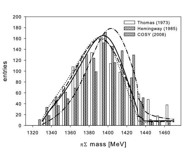
Figure 3: The $\pi\Sigma$ mass distribution. Our results are compared with the experimental data taken from Refs. [32], [33] and [34]. The full line was obtained for the parameter set of the present work, the dashed line for the one of Ref. [22], both related to $\sigma_{\pi N}=40$ MeV. See the text for explanation on the dotted and dash-dotted lines.

The experimental data shown in Fig. 3 come from three different measurements [32], [33], [34], all exhibiting a prominent structure around 1400 MeV. As the observed spectra are not normalized we have rescaled the original data as well as our computed distributions to give 1000 events in the chosen energy interval (from 1330 to 1440 MeV). The three measurements give $\pi\Sigma$ distributions that look mutually compatible. We have not included in the figure the $K^{-}p\rightarrow\Sigma^{0}\pi^{0}\pi^{0}$ data measured by the Crystal Ball Collaboration [16] as they yield a slightly different distribution with a peak structure around 1420 MeV. The two identical pions in the final state of the later reaction complicate a comparison with the other experiments, so we find it questionable to relate our computed lineshape to the one observed in [16] without employing fully the dynamics of the particular reaction as it was done in [15].

The values of $r_{KN/\pi\Sigma}$ obtained in our fits (and presented in the Table 4) are compatible with similar findings by other authors [14], [7]. Since the magnitude of $r_{KN/\pi\Sigma}$ is of the order of one it looks that both the $\bar{K}N$ and the $\pi\Sigma$ states contribute to the $I=0$ resonance identified with $\Lambda(1405)$ with a comparable strength. In other words, the inclusion of the initial $\bar{K}N$ channels in the model driven by Eq. (13) is important. This is fully in line with the well known fact that the $\Lambda(1405)$ resonance does couple strongly to the $K^{-}p$ state. Unfortunately, the experimental data are not precise enough to distinguish between various values of $r_{KN/\pi\Sigma}$ which is demonstrated in Fig. 3 by comparing our best fit results with those generated for the boundary values of $r_{KN/\pi\Sigma}$. Since a good description of the spectrum can already be achieved without its inclusion in the fits one may argue that the dynamics of the chiral model is fixed by the threshold (and low energy) observables of $K^{-}p$ interactions. However, the data clearly prefer a positive sign of $r_{KN/\pi\Sigma}$, i.e. a constructive interference of the contributions provided by the $\pi\Sigma$ and $\bar{K}N$ channels to the resonance. For the negative values of $r_{KN/\pi\Sigma}$ the peak moves to energies lower than the one obtained at the $r_{KN/\pi\Sigma}=0$ boundary and the computed spectrum no longer matches the experimental one.

Table 4: The complex energies of the poles relevant to the $I=0$ resonance.

$\sigma_{\pi N}$ [MeV]	$r_{KN/\pi\Sigma}$	Re $z_{1}$ [MeV]	Im $z_{1}$ [MeV]	Re $z_{2}$ [MeV]	Im $z_{2}$ [MeV]
20	1.28	1395	-49	1456	-77
30	1.32	1398	-51	1441	-76
40	0.37	1401	-41	1519	-112
50	0.54	1406	-39	1436	-138

The interest in the $\pi\Sigma$ mass distribution has arisen since discovering that the chiral meson-baryon dynamics generates two poles in the complex energy plane that can be related to the $\Lambda(1405)$ resonance. In the Table 4 we show the positions of the poles generated by our model. They appear on the unphysical Riemann sheet accessed when crossing the real axis between the thresholds of the $\pi\Sigma$ and the $\bar{K}N$ channels. The position of the lower (with the lower value of the real part of the complex energy) pole is moreless stable and does not depend much on the choice of the parameter set. Its complex energy $z\approx 1400-{\rm i}\>45$ MeV can clearly be associated with the observed $\pi\Sigma$ mass spectrum. On the other hand, the higher (in terms of Re $z$) pole is located further from the real axis and its position vary with the chosen parameter set. We have also noted that parameter sets obtained for various local $\chi^{2}$ minima lead to different positions of this pole even if they correspond to the same choice of the $\pi N$ sigma term.

Interestingly, neither of the two poles is located so close to the real energy axis as other authors claim. This feature can be explained by a different parametrization of our model. It was already shown by Borasoy et al. [7] that the second pole moves away from the real axis when the second order terms are included in the chiral Lagrangian. Our observations confirm this. When we performed a fit (for $\sigma_{\pi N}=40$ MeV) with the next-to-leading order terms neglected we located the poles at $z_{1}=(1368-{\rm i}\>42)$ MeV and $z_{2}=(1441-{\rm i}\>22)$ MeV. Although the second pole remains above the $\bar{K}N$ threshold while other authors observe it about 10 MeV below the threshold, the closeness of the pole to the real axis seems to be related to the omission of the next-to-leading order corrections in the chiral Lagrangian. We also noted that our fits with interaction restricted only to the Weinberg-Tomozawa term require very large values of the parameter $r_{KN/\pi\Sigma}$, typically $r_{KN/\pi\Sigma}\mathchoice{\mathrel{\vbox{\hbox{$\buildrel\displaystyle>\over{\displaystyle\sim}$}}}}{\mathrel{\vbox{\hbox{$\buildrel\textstyle>\over{\textstyle\sim}$}}}}{\mathrel{\vbox{\hbox{$\buildrel\scriptstyle>\over{\scriptstyle\sim}$}}}}{\mathrel{\vbox{\hbox{$\buildrel\scriptscriptstyle>\over{\scriptscriptstyle\sim}$}}}}10$. This means that in such a case the resonance observed in the $\pi\Sigma$ mass spectrum couples much stronger to the $\bar{K}N$ channels than to the $\pi\Sigma$ ones.

Though the quality of the fit is much worse without the second order terms (we got $\chi^{2}/N=3.1$ in the case mentioned here), most of the $K^{-}p$ data are still reproduced quite well. On the other hand Hyodo and Weise [35], who locate the $\bar{K}N$ quasibound state at $\sqrt{s}\simeq 1420$ MeV, use a parametrization that is not suitable for a description of all relevant $\bar{K}N$ data, specifically they do not reproduce (as one can check in [36]) the precise threshold rates, Eq. (12). Borasoy et al. [7] do fit all relevant $K^{-}p$ data including the threshold rates, however their pole at 1420 MeV moves away from the real axis (and to lower energies) when they include the DEAR data in their fits. When they compromise the DEAR data with those from $K^{-}p$ reactions they get the pole quite close to where we see it. Therefore, it looks plausible that the remaining differences in exact localization of the poles can be attributed either to model specifics or to the fact that the models do not reproduce all observed experimental data on the same footing. In a comment made by one of us and A. Gal [37] we also showed that the position of the poles can change drastically when playing with the meson-baryon channel couplings. Thus, it should not be surprising that different parametrizations of the chiral model lead to different pole positions.

The shape of the $\pi\Sigma$ mass spectrum is determined by the positions of the two $I=0$ poles and by the relative couplings of the $\pi\Sigma$ and $\bar{K}N$ states to the poles (the parameter $r_{KN/\pi\Sigma}$ in our model). It is obvious that the observed spectrum does not resemble a typical Breit-Wigner resonance. While this can be attributed to an interplay of two resonances that are relatively close to the real axis [14] we can explain the $\pi\Sigma$ distribution without any resonance that sits in a vicinity of the real axis. In our model the observed structure is not of the Breit-Wigner type simply because there is no pole sufficiently close to the real axis. We hope that new results from experiments dedicated to exploration of the $\Lambda(1405)$ structure will be able to distinguish between those two pictures.

4.3 $K^{-}n$ amplitude

Once the low-energy constants of the chiral Lagrangian, Eqs. (6) and (3), and the inverse ranges of meson-baryon interactions are fixed to the $K^{-}p$ data the model provides us with predictions for other interactions of the meson octet with the baryonic one. Here we discuss our results for the meson-baryon systems with total charge $Q=-1$, specifically for the $K^{-}n$ amplitude. In the $Q=-1$ sector the coupled channels are represented by the following ones: $K^{-}\Lambda$, $\pi^{-}\Sigma^{0}$, $\pi^{0}\Sigma^{-}$, $K^{-}n$, $\eta\Sigma^{-}$, $K^{0}\Xi^{-}$ (listed and numbered according to the respective thresholds). Exactly as in the $Q=0$ sector related to the $K^{-}p$ system we construct the effective potentials (1) with the coupling matrix $C_{ij}$ given in Appendix B.

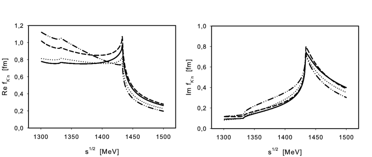
Figure 4: The real (left panel) and imaginary (right panel) parts of the $K^{-}n$ amplitude. The full, dotted, dashed and dot-dashed lines visualize our results obtained with the parameter sets corresponding to $\sigma_{\pi N}$ terms set to 20, 30, 40 and 50 MeV, respectively.

In Figure 4 we present our results for the elastic $K^{-}n$ amplitude as a function of the c.m.s. energy. It is a bit surprising to see how much the calculated amplitudes depend on the choice of the parameter set (related to the value of the $\sigma_{\pi N}$ term). We have demonstrated that all four choices give an equivalent description of the available $K^{-}p$ data, so one would expect a similar feature in the $K^{-}n$ sector as well. This is not true either at the $\bar{K}N$ threshold or below it. At the $K^{-}n$ threshold the variations in the real part of the elastic amplitude make as much as some 30%. It is also worth noting that for energies below the threshold the real part of the $K^{-}n$ amplitude follows a different trend than the one reported in Refs. [7] and [35]. Specifically, our Re $f_{K^{-}n}$ is either a slightly decreasing or a moreless constant function of the energy while in [7] and [35] it turned out as monotonically increasing function of energy below the threshold. While the authors of the first paper [7] work with the physical meson and baryon masses and their approach is similar to ours (parameters fitted to $K^{-}p$ data used to compute the $K^{-}n$ amplitude) the results of the more recent work by Hyodo and Weise [35] were obtained in a model that adopts fully the isospin symmetry and does not aim at a realistic description of the $K^{-}p$ threshold branching ratios. Since the other authors do not incorporate off-shell effects and use a different formulation of the $\bar{K}N$ dynamics it is difficult to trace the origin of the observed differences. We have checked that the inclusion of the ”u” terms (corresponding to Fig. 1d) in the calculation (which the other authors refrained from) leads only to a minor modification of the $K^{-}n$ amplitude below the threshold. We demonstrate the effect in Figure 5 where the full line represents the present calculation completed with all terms included and the dotted line corresponds to the calculation without the ”u” terms. For the real part of the amplitude both lines moreless coincide at energies above the $K^{-}n$ threshold. The dashed line represents the results obtained for the parameter set of Ref. [22], our previous fit to the $K^{-}p$ data performed without any restrictions on the inverse ranges $\alpha_{j}$. Since the full and dashed lines correspond to two different $\chi^{2}$ minima (but to the same choice of the $\sigma_{\pi N}$) the lineshape variations give an idea of the theoretical uncertainies inherent in our description of the $K^{-}n$ amplitude.

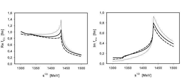
Figure 5: The real (left panel) and imaginary (right panel) parts of the $K^{-}n$ amplitude. Results are presented only for the parameter set corresponding to $\sigma_{\pi N}=40$ MeV. See text for more details.

In principle, the elastic $K^{-}n$ amplitude can be related to the isovector parts of the $\bar{K}N$ amplitudes obtained in the $Q=0$ sector, i.e. for the coupled channel model used to describe the $K^{-}p$ data. However, the physical meson and baryon masses break the isospin symmetry and the threshold energies of different $\bar{K}N$ channels are different too. Thus, one should be careful when using the isospin relations at or near the $\bar{K}N$ thresholds. To demonstrate the ambiguity, in Figure 6 we present a comparison of the elastic $K^{-}p$ and $\bar{K}^{0}n$ amplitudes. Although both amplitudes have the same isospin content, their behaviour at threshold energies is quite different.

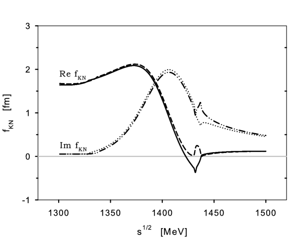
Figure 6: The energy dependence of the $K^{-}p$ and $\bar{K}^{0}n$ elastic amplitudes. The real and imaginary parts of the amplitudes are shown in the same figure with the full and dotted lines used for the $K^{-}p$ amplitude and the dashed and dot-dashed lines used for the $\bar{K}^{0}n$ amplitude, respectively.

In effect, the $K^{-}n$ amplitude derived by means of isospin relations depends on the isospin scheme. We found that it is vital to use the average of both, the $K^{-}p$ and $\bar{K}^{0}n$ amplitudes, rather then only one of them (normally the $K^{-}p$ one as there are relevant experimental data). We demonstrate the point in Figure 7 where the $K^{-}n$ amplitudes obtained by means of two different isospin schemes are compared with our direct (six coupled channels) calculation. The dotted lines in the figure correspond to the scheme in which the $K^{-}n$ amplitude is derived from the elastic $K^{-}p$ amplitude and from the transition amplitude of the $K^{-}p\rightarrow\bar{K}^{0}n$ process,

$$\langle K^{-}n|f|K^{-}n\rangle=\langle K^{-}p|f|K^{-}p\rangle-\langle\bar{K}^{0}n|f|K^{-}p\rangle\;.$$ (20)

One immediately notes the unphysical oscillations in-between the $K^{-}p$ and $\bar{K}^{0}n$ thresholds. This can be remedied by taking the average of both the elastic $K^{-}p$ and $\bar{K}^{0}n$ amplitudes, i.e. by replacing Eq.(20) with

$$\langle K^{-}n|f|K^{-}n\rangle=(\langle K^{-}p|f|K^{-}p\rangle+\langle\bar{K}^{0}n|f|\bar{K}^{0}n\rangle)/2-\langle\bar{K}^{0}n|f|K^{-}p\rangle\;.$$ (21)

The resulting $K^{-}n$ amplitude is given by the dashed line in Fig. 7. As this approach does not lead to unphysical oscillations it should be prefered in any relevant analysis. This scheme is also consistent with the construction of the transition amplitudes between the $\bar{K}N$ states of specific isospins when they are decomposed into pertinent physical channels. Of course, the dashed lines still exhibit cusps at the $K^{-}p$ and $\bar{K}^{0}n$ thresholds and differ slightly from the full lines that represent the direct calculation of the $K^{-}n$ amplitude (with only one threshold cusp at the physicaly correct energy). As expected, the effects related to the isospin violation are observed only in the region of the $\bar{K}N$ thresholds and the lines practically coincide at energies sufficiently far from the thresholds.

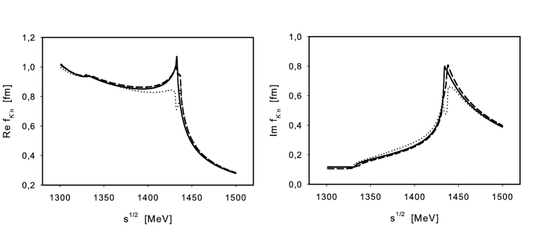
Figure 7: Comparison of two different isospin schemes with the direct calculation of the $K^{-}n$ amplitude. The real and imaginary parts of the amplitude are shown in the left and right panels, respectively. See text for more details.

5 Conclusions

An effective chirally motivated separable potential was used in simultaneous fits of the low energy $K^{-}p$ cross sections, the threshold branching ratios and the characteristics of kaonic hydrogen. The fits are quite satisfactory except for the 1s level decay width being much larger than the experimental value. We have computed the characteristics of kaonic hydrogen (the 1s level energy shift and width) exactly and emphasize that this approach is vital in view of the expected precision of the coming experimental data.

Our results confirm observations by other authors that the coupled channel chiral model leads to two poles in the complex energy plane that can be related to the $\Lambda(1405)$ resonance observed in the $\pi\Sigma$ mass spectrum. However, we are not so convinced that both poles affect the physical observables as their positions seem to be model dependent and especially the one at higher energies may easily drift too far from the real axis. It is also intriguing that we were not able to get the position of any of the poles so close to the real axis as other authors claim. The disparity can be attributed most likely to the inclusion of the $q^{2}$ terms in the chiral Lagrangian and partly also to a different formulation of our model, namely to the use of effective separable potentials instead of the on-shell scheme employed in the inverse T-matrix approach.

We have also shown that near the $\bar{K}N$ threshold the $K^{-}n$ amplitude obtained from multiple channel calculations with physical particle masses differs from the one derived by means of isospin relations from the transition amplitudes obtained in the $K^{-}p$ sector. Despite the underlying chiral Lagrangian adheres to the SU(3) symmetry and incorporates fully the isospin symmetry the use of physical masses breaks the symmetry. As the thresholds of the $K^{-}p$, $K^{-}n$ and $\bar{K}^{0}n$ channels are different one cannot simply relate the $K^{-}n$ amplitude to those from the $K^{-}p$ sector. Our results clearly demonstrate this and show that both elastic $K^{-}N$ amplitudes exhibit a strong energy dependence in the vicinity of $\bar{K}N$ thresholds. It also means that it may not be easy and straightforward to relate the $K^{-}$-deuteron scattering length to the $K^{-}N$ ones observed in experiments.

We close the paper by expressing a hope that the forthcoming high-precision data from the DEAR/SIDDHARTA collaboration and from experiments dedicated to the $\Lambda(1405)$ resonance will shred more light on kaon-nucleon dynamics and stimulate further theoretical work.

Acknowledgement: The authors acknowledge the financial support from the Grant Agency of the Czech Republic, grant 202/09/1441. The work of J. S. was also supported by the Research Program Fundamental experiments in the physics of the microworld No. 6840770040 of the Ministry of Education, Youth and Sports of the Czech Republic.

Appendix A

In the appendices we specify the coefficients $C_{ij}^{\rm(.)}$ of Eq. (11). First we present the matrices for the channels coupled to the $K^{-}p$ ($Q=0$ and $S=1$ meson-baryon system), the following Appendix B is reserved for the channels coupled to the $K^{-}n$ ($Q=-1$ and $S=1$). As the coupling matrices are symmetric, $C_{ji}^{\rm(.)}=\,C_{ij}^{\rm(.)}$, we show only the terms above the diagonal and cut most tables in two parts to save some space. For the later reason we also split the table for the coefficients $C_{ij}^{(EE)}$ in two, so one should sum the respective terms, $C_{ij}^{(EE)}=C_{ij}^{(EE1)}+C_{ij}^{(EE2)}$.

Table A1: $K^{-}p$ related channels - the (WT) term coefficients. $C_{ji}^{\rm(WT)}=\,C_{ij}^{\rm(WT)}$.

	$\pi^{0}\Lambda$	$\pi^{0}\Sigma^{0}$	$\pi^{-}\Sigma^{+}$	$\pi^{+}\Sigma^{-}$	$K^{-}p$	$\bar{K}^{0}n$	$\eta\Lambda$	$\eta\Sigma^{0}$	$K^{0}\Xi^{0}$	$K^{+}\Xi^{-}$
$\pi^{0}\Lambda$	0	0	0	0	$\frac{\sqrt{3}}{2}$	$-\frac{\sqrt{3}}{2}$	0	0	$-\frac{\sqrt{3}}{2}$	$\frac{\sqrt{3}}{2}$
$\pi^{0}\Sigma^{0}$		0	2	2	$\frac{1}{2}$	$\frac{1}{2}$	0	0	$\frac{1}{2}$	$\frac{1}{2}$
$\pi^{-}\Sigma^{+}$			2	0	1	0	0	0	1	0
$\pi^{+}\Sigma^{-}$				2	0	1	0	0	0	1
$K^{-}p$					2	1	$\frac{3}{2}$	$\frac{\sqrt{3}}{2}$	0	0
$\bar{K}^{0}n$						2	$\frac{3}{2}$	$-\frac{\sqrt{3}}{2}$	0	0
$\eta\Lambda$							0	0	$\frac{3}{2}$	$\frac{3}{2}$
$\eta\Sigma^{0}$								0	$-\frac{\sqrt{3}}{2}$	$\frac{\sqrt{3}}{2}$
$K^{0}\Xi^{0}$									2	1
$K^{+}\Xi^{-}$										2

Table A2: $K^{-}p$ related channels - the (mm) term coefficients. $C_{ji}^{(mm)}=\,C_{ij}^{(mm)}$.

	$\pi^{0}\Lambda$	$\pi^{0}\Sigma^{0}$	$\pi^{-}\Sigma^{+}$	$\pi^{+}\Sigma^{-}$	$K^{-}p$
$\pi^{0}\Lambda$	$\frac{2}{3}(3b_{0}+b_{\rm D})$	0	0	0	$-\frac{\sqrt{3}}{6}(b_{\rm D}+3b_{\rm F})$
$\pi^{0}\Sigma^{0}$		$2(b_{0}+b_{\rm D})$	0	0	$\frac{1}{2}(b_{\rm D}-b_{\rm F})$
$\pi^{-}\Sigma^{+}$			$2(b_{0}+b_{\rm D})$	0	$(b_{\rm D}-b_{\rm F})$
$\pi^{+}\Sigma^{-}$				$2(b_{0}+b_{\rm D})$	0
$K^{-}p$					$2(b_{0}+b_{\rm D})$
	$\bar{K}^{0}n$	$\eta\Lambda$	$\eta\Sigma^{0}$	$K^{0}\Xi^{0}$	$K^{+}\Xi^{-}$
$\pi^{0}\Lambda$	$\frac{\sqrt{3}}{6}(b_{\rm D}+3b_{\rm F})$	0	$\frac{2}{3}b_{\rm D}$	$\frac{\sqrt{3}}{6}(b_{\rm D}-3b_{\rm F})$	$-\frac{\sqrt{3}}{6}(b_{\rm D}-3b_{\rm F})$
$\pi^{0}\Sigma^{0}$	$\frac{1}{2}(b_{\rm D}-b_{\rm F})$	$\frac{2}{3}b_{\rm D}$	0	$\frac{1}{2}(b_{\rm D}+b_{\rm F})$	$\frac{1}{2}(b_{\rm D}+b_{\rm F})$
$\pi^{-}\Sigma^{+}$	0	$\frac{2}{3}b_{\rm D}$	$-\frac{2\sqrt{3}}{3}b_{\rm F}$	$(b_{\rm D}+b_{\rm F})$	0
$\pi^{+}\Sigma^{-}$	$(b_{\rm D}-b_{\rm F})$	$\frac{2}{3}b_{\rm D}$	$\frac{2\sqrt{3}}{3}b_{\rm F}$	0	$(b_{\rm D}+b_{\rm F})$
$K^{-}p$	$(b_{\rm D}+b_{\rm F})$	$\frac{1}{6}(b_{\rm D}+3b_{\rm F})$	$-\frac{\sqrt{3}}{6}(b_{\rm D}-b_{\rm F})$	0	0
$\bar{K}^{0}n$	$2(b_{0}+b_{\rm D})$	$\frac{1}{6}(b_{\rm D}+3b_{\rm F})$	$\frac{\sqrt{3}}{6}(b_{\rm D}-b_{\rm F})$	0	0
$\eta\Lambda$		$2(b_{0}+b_{\rm D})$	0	$\frac{1}{6}(b_{\rm D}-3b_{\rm F})$	$\frac{1}{6}(b_{\rm D}-3b_{\rm F})$
$\eta\Sigma^{0}$			$\frac{2}{3}(3b_{0}+b_{\rm D})$	$\frac{\sqrt{3}}{6}(b_{\rm D}+b_{\rm F})$	$-\frac{\sqrt{3}}{6}(b_{\rm D}+b_{\rm F})$
$K^{0}\Xi^{0}$				$2(b_{0}+b_{\rm D})$	$(b_{\rm D}-b_{\rm F})$
$K^{+}\Xi^{-}$					$2(b_{0}+b_{\rm D})$

Table A3: $K^{-}p$ related channels - the $(\chi{\rm b})$ term coefficients. Only the ”lower” part of the table is shown. All coefficients in the ”upper” part (terms above the diagonal in columns from $\pi^{0}\Lambda$ to $K^{-}p$) are equal to zero. $C_{ji}^{(\chi{\rm b})}=\,C_{ij}^{(\chi{\rm b})}$.

	$\bar{K}^{0}n$	$\eta\Lambda$	$\eta\Sigma^{0}$	$K^{0}\Xi^{0}$	$K^{+}\Xi^{-}$
$\pi^{0}\Lambda$	0	$\frac{4}{9}(b_{\rm D}+3b_{\rm F})$	-$\frac{4\sqrt{3}}{9}(b_{\rm D}-b_{\rm F})$	0	0
$\pi^{0}\Sigma^{0}$	0	-$\frac{8}{9}b_{\rm D}$	0	0	0
$\pi^{-}\Sigma^{+}$	0	$-\frac{8}{9}b_{\rm D}$	$\frac{8\sqrt{3}}{9}b_{\rm F}$	0	0
$\pi^{+}\Sigma^{-}$	0	$-\frac{8}{9}b_{\rm D}$	$-\frac{8\sqrt{3}}{9}b_{\rm F}$	0	0
$K^{-}p$	0	$\frac{4}{9}(b_{\rm D}+3b_{\rm F})$	$-\frac{4\sqrt{3}}{9}(b_{\rm D}-b_{\rm F})$	0	0
$\bar{K}^{0}n$	0	$\frac{4}{9}(b_{\rm D}+3b_{\rm F})$	$\frac{4}{9}(b_{\rm D}-b_{\rm F})$	0	0
$\eta\Lambda$		$\frac{16}{9}b_{\rm D}$	0	$\frac{4}{9}(b_{\rm D}-3b_{\rm F})$	$\frac{4}{9}(b_{\rm D}-3b_{\rm F})$
$\eta\Sigma^{0}$			$-\frac{16}{9}b_{\rm D}$	$\frac{4\sqrt{3}}{9}(b_{\rm D}+b_{\rm F})$	$-\frac{4\sqrt{3}}{9}(b_{\rm D}+b_{\rm F})$
$K^{0}\Xi^{0}$				0	0
$K^{+}\Xi^{-}$					0

Table A4: $K^{-}p$ related channels - the (EE1) term coefficients. $C_{ji}^{(EE1)}=C_{ij}^{(EE1)}$.

	$\pi^{0}\Lambda$	$\pi^{0}\Sigma^{0}$	$\pi^{-}\Sigma^{+}$	$\pi^{+}\Sigma^{-}$	$K^{-}p$
$\pi^{0}\Lambda$	$-\frac{2}{3}(3d_{0}+d_{\rm D})$	0	0	0	$\frac{\sqrt{3}}{6}(d_{\rm D}+3d_{\rm F})$
$\pi^{0}\Sigma^{0}$		$-2(d_{0}+d_{\rm D})$	0	0	$-\frac{1}{2}(d_{\rm D}-d_{\rm F})$
$\pi^{-}\Sigma^{+}$			$-2(d_{0}+d_{\rm D})$	0	$-(d_{\rm D}-d_{\rm F})$
$\pi^{+}\Sigma^{-}$				$-2(d_{0}+d_{\rm D})$	0
$K^{-}p$					$-2(d_{0}+d_{\rm D})$
	$\bar{K}^{0}n$	$\eta\Lambda$	$\eta\Sigma^{0}$	$K^{0}\Xi^{0}$	$K^{+}\Xi^{-}$
$\pi^{0}\Lambda$	$-\frac{\sqrt{3}}{6}(d_{\rm D}+3d_{\rm F})$	0	$-\frac{2}{3}d_{\rm D}$	$-\frac{\sqrt{3}}{6}(d_{\rm D}-3d_{\rm F})$	$\frac{\sqrt{3}}{6}(d_{\rm D}-3d_{\rm F})$
$\pi^{0}\Sigma^{0}$	$-\frac{1}{2}(d_{\rm D}-d_{\rm F})$	$-\frac{2}{3}d_{\rm D}$	0	$-\frac{1}{2}(d_{\rm D}+d_{\rm F})$	$-\frac{1}{2}(d_{\rm D}+d_{\rm F})$
$\pi^{-}\Sigma^{+}$	0	$-\frac{2}{3}d_{\rm D}$	$\frac{2\sqrt{3}}{3}d_{\rm F}$	$-(d_{\rm D}+d_{\rm F})$	0
$\pi^{+}\Sigma^{-}$	$-(d_{\rm D}-d_{\rm F})$	$-\frac{2}{3}d_{\rm D}$	$-\frac{2\sqrt{3}}{3}d_{\rm F}$	0	$-(d_{\rm D}+d_{\rm F})$
$K^{-}p$	$-(d_{\rm D}+d_{\rm F})$	$-\frac{1}{6}(d_{\rm D}+3d_{\rm F})$	$\frac{\sqrt{3}}{6}(d_{\rm D}-d_{\rm F})$	0	0
$\bar{K}^{0}n$	$-2(d_{0}+d_{\rm D})$	$-\frac{1}{6}(d_{\rm D}+3d_{\rm F})$	$-\frac{\sqrt{3}}{6}(d_{\rm D}-d_{\rm F})$	0	0
$\eta\Lambda$		$-2(d_{0}+d_{\rm D})$	0	$-\frac{1}{6}(d_{\rm D}-3d_{\rm F})$	$-\frac{1}{6}(d_{\rm D}-3d_{\rm F})$
$\eta\Sigma^{0}$			$-\frac{2}{3}(3d_{0}+d_{\rm D})$	$-\frac{\sqrt{3}}{6}(d_{\rm D}+d_{\rm F})$	$\frac{\sqrt{3}}{6}(d_{\rm D}+d_{\rm F})$
$K^{0}\Xi^{0}$				$-2(d_{0}+d_{\rm D})$	$-(d_{\rm D}-d_{\rm F})$
$K^{+}\Xi^{-}$					$-2(d_{0}+d_{\rm D})$

Table A5: $K^{-}p$ related channels - the (EE2) term coefficients. $C_{ji}^{(EE2)}=C_{ij}^{(EE2)}$.

	$\pi^{0}\Lambda$	$\pi^{0}\Sigma^{0}$	$\pi^{-}\Sigma^{+}$	$\pi^{+}\Sigma^{-}$	$K^{-}p$
$\pi^{0}\Lambda$	$-\frac{1}{3}d_{2}$	0	0	0	$-\frac{\sqrt{3}}{6}d_{2}$
$\pi^{0}\Sigma^{0}$		$-2d_{1}-d_{2}$	$-d_{1}-d_{2}$	$-d_{1}-d_{2}$	$-d_{1}-\frac{1}{2}d_{2}$
$\pi^{-}\Sigma^{+}$			$-d_{1}$	$-2d_{1}-2d_{2}$	$-d_{1}$
$\pi^{+}\Sigma^{-}$				$-d_{1}$	$-d_{1}-d_{2}$
$K^{-}p$					$-d_{1}$
	$\bar{K}^{0}n$	$\eta\Lambda$	$\eta\Sigma^{0}$	$K^{0}\Xi^{0}$	$K^{+}\Xi^{-}$
$\pi^{0}\Lambda$	$\frac{\sqrt{3}}{6}d_{2}$	0	$-d_{1}-\frac{1}{3}d_{2}$	$\frac{\sqrt{3}}{6}d_{2}$	$-\frac{\sqrt{3}}{6}d_{2}$
$\pi^{0}\Sigma^{0}$	$-d_{1}-\frac{1}{2}d_{2}$	$-d_{1}-\frac{1}{3}d_{2}$	0	$-d_{1}-\frac{1}{2}d_{2}$	$-d_{1}-\frac{1}{2}d_{2}$
$\pi^{-}\Sigma^{+}$	$-d_{1}-d_{2}$	$-d_{1}-\frac{1}{3}d_{2}$	0	$-d_{1}$	$-d_{1}-d_{2}$
$\pi^{+}\Sigma^{-}$	$-d_{1}$	$-d_{1}-\frac{1}{3}d_{2}$	0	$-d_{1}-d_{2}$	$-d_{1}$
$K^{-}p$	$-d_{1}$	$-d_{1}-\frac{5}{6}d_{2}$	$-\frac{\sqrt{3}}{6}d_{2}$	$-d_{1}-d_{2}$	$-2(d_{1}+d_{2})$
$\bar{K}^{0}n$	$-d_{1}$	$-d_{1}-\frac{5}{6}d_{2}$	$\frac{\sqrt{3}}{6}d_{2}$	$-2(d_{1}+d_{2})$	$-d_{1}-d_{2}$
$\eta\Lambda$		$-2d_{1}-d_{2}$	0	$-d_{1}-\frac{5}{6}d_{2}$	$-d_{1}-\frac{5}{6}d_{2}$
$\eta\Sigma^{0}$			$-\frac{1}{3}d_{2}$	$\frac{\sqrt{3}}{6}d_{2}$	$-\frac{\sqrt{3}}{6}d_{2}$
$K^{0}\Xi^{0}$				$-d_{1}$	$-d_{1}$
$K^{+}\Xi^{-}$					$-d_{1}$

Table A6: $K^{-}p$ related channels - the direct (s) term coefficients. $C_{ji}^{(s)}=C_{ij}^{(s)}$.

	$\pi^{0}\Lambda$	$\pi^{0}\Sigma^{0}$	$\pi^{-}\Sigma^{+}$	$\pi^{+}\Sigma^{-}$	$K^{-}p$
$\pi^{0}\Lambda$	$-\frac{1}{3}D^{2}$	0	$-\frac{\sqrt{3}}{3}DF$	$\frac{\sqrt{3}}{3}DF$	$\frac{\sqrt{3}}{6}(D^{2}\!-\!DF)$
$\pi^{0}\Sigma^{0}$		$\frac{1}{3}D^{2}$	$\frac{1}{3}D^{2}$	$\frac{1}{3}D^{2}$	$-\frac{1}{6}D^{2}\!-\!\frac{1}{2}DF$
$\pi^{-}\Sigma^{+}$			$\frac{1}{3}D^{2}+F^{2}$	$\frac{1}{3}D^{2}-F^{2}$	$-\frac{1}{6}D^{2}\!-\!DF\!+\!\frac{1}{2}F^{2}$
$\pi^{+}\Sigma^{-}$				$\frac{1}{3}D^{2}\!+\!F^{2}$	$-\frac{1}{6}D^{2}\!-\!\frac{1}{2}F^{2}$
$K^{-}p$					$\frac{1}{3}D^{2}\!+\!F^{2}$
	$\bar{K}^{0}n$	$\eta\Lambda$	$\eta\Sigma^{0}$	$K^{0}\Xi^{0}$	$K^{+}\Xi^{-}$
$\pi^{0}\Lambda$	$-\frac{\sqrt{3}}{6}(D^{2}\!-\!DF)$	0	$\frac{1}{3}D^{2}$	$-\frac{\sqrt{3}}{6}(D^{2}\!+\!DF)$	$\frac{\sqrt{3}}{6}(D^{2}\!+\!DF)$
$\pi^{0}\Sigma^{0}$	$-\frac{1}{6}(D^{2}\!+\!3DF)$	$-\frac{1}{3}D^{2}$	0	$-\frac{1}{6}(D^{2}\!-\!3DF)$	$-\frac{1}{6}(D^{2}\!-\!3DF)$
$\pi^{-}\Sigma^{+}$	$-\frac{1}{6}(D^{2}\!+\!3F^{2})$	$-\frac{1}{3}D^{2}$	$-\frac{\sqrt{3}}{3}DF$	$-\frac{1}{6}D^{2}\!+\!\frac{1}{2}F^{2}\!+\!DF$	$-\frac{1}{6}(D^{2}\!+\!3F^{2})$
$\pi^{+}\Sigma^{-}$	$-\frac{1}{6}D^{2}\!+\!\frac{1}{2}F^{2}\!-\!DF$	$-\frac{1}{3}D^{2}$	$\frac{\sqrt{3}}{3}DF$	$-\frac{1}{6}(D^{2}\!+\!3F^{2})$	$-\frac{1}{6}D^{2}\!+\!\frac{1}{2}F^{2}\!+\!DF$
$K^{-}p$	$-\frac{1}{6}D^{2}\!+\!\frac{1}{2}F^{2}\!+\!DF$	$\frac{1}{6}(D^{2}\!+\!3DF)$	$\frac{\sqrt{3}}{6}(D^{2}\!-\!DF)$	$-\frac{1}{6}(D^{2}\!+\!3F^{2})$	$\frac{1}{3}(D^{2}\!-\!3F^{2})$
$\bar{K}^{0}n$	$\frac{1}{3}(D^{2}\!+\!3F^{2})$	$\frac{1}{6}(D^{2}\!+\!3DF)$	$-\frac{\sqrt{3}}{6}(D^{2}\!-\!DF)$	$\frac{1}{3}(D^{2}\!-\!3F^{2})$	$-\frac{1}{6}(D^{2}\!+\!3F^{2})$
$\eta\Lambda$		$\frac{1}{3}D^{2}$	0	$\frac{1}{6}(D^{2}\!-\!3DF)$	$\frac{1}{6}(D^{2}\!-\!3DF)$
$\eta\Sigma^{0}$			$\frac{1}{3}D^{2}$	$-\frac{\sqrt{3}}{6}(D^{2}\!+\!DF)$	$\frac{\sqrt{3}}{6}(D^{2}\!+\!DF)$
$K^{0}\Xi^{0}$				$\frac{1}{3}(D^{2}\!+\!3F^{2})$	$-\frac{1}{6}D^{2}\!+\!\frac{1}{2}F^{2}\!-\!DF$
$K^{+}\Xi^{-}$					$\frac{1}{3}(D^{2}\!+\!3F^{2})$

Table A7: $K^{-}p$ related channels - the crossed (u) term coefficients. $C_{ji}^{(u)}=C_{ij}^{(u)}$. To shorten the length of some coefficients we denote ${\cal U}_{+++}=\frac{\sqrt{3}}{12}D^{2}+\frac{\sqrt{3}}{4}F^{2}+\frac{\sqrt{3}}{3}DF$ and use ${\cal U}_{abc}$ with $a$, $b$ and $c$ marking the signs of the terms with $D^{2}$, $F^{2}$ and $DF$, respectively.

	$\pi^{0}\Lambda$	$\pi^{0}\Sigma^{0}$	$\pi^{-}\Sigma^{+}$	$\pi^{+}\Sigma^{-}$	$K^{-}p$
$\pi^{0}\Lambda$	$\frac{1}{3}D^{2}$	0	$\frac{\sqrt{3}}{3}DF$	$-\frac{\sqrt{3}}{3}DF$	${\cal U}_{---}$
$\pi^{0}\Sigma^{0}$		$\frac{1}{3}D^{2}$	$-F^{2}$	$-F^{2}$	$\frac{1}{4}(D^{2}-F^{2})$
$\pi^{-}\Sigma^{+}$			0	$\frac{1}{3}D^{2}-F^{2}$	0
$\pi^{+}\Sigma^{-}$				0	$\frac{1}{2}(D^{2}-F^{2})$
$K^{-}p$					0
	$\bar{K}^{0}n$	$\eta\Lambda$	$\eta\Sigma^{0}$	$K^{0}\Xi^{0}$	$K^{+}\Xi^{-}$
$\pi^{0}\Lambda$	${\cal U}_{+++}$	0	$-\frac{1}{3}D^{2}$	${\cal U}_{++-}$	${\cal U}_{--+}$
$\pi^{0}\Sigma^{0}$	$\frac{1}{4}(D^{2}-F^{2})$	$\frac{1}{3}D^{2}$	0	$\frac{1}{4}(D^{2}-F^{2})$	$\frac{1}{4}(D^{2}-F^{2})$
$\pi^{-}\Sigma^{+}$	$\frac{1}{2}(D^{2}-F^{2})$	$-\frac{1}{3}D^{2}$	$-\frac{\sqrt{3}}{3}DF$	0	$\frac{1}{2}(D^{2}-F^{2})$
$\pi^{+}\Sigma^{-}$	0	$\frac{1}{3}D^{2}$	$\frac{\sqrt{3}}{3}DF$	$\frac{1}{2}(D^{2}-F^{2})$	0
$K^{-}p$	0	$\frac{1}{12}(D^{2}-9F^{2})$	${\cal U}_{--+}$	$\frac{1}{2}(D^{2}-F^{2})$	$\frac{1}{3}(D^{2}-3F^{2})$
$\bar{K}^{0}n$	0	$\frac{1}{12}(D^{2}-9F^{2})$	${\cal U}_{++-}$	$\frac{1}{3}(D^{2}-3F^{2})$	$\frac{1}{2}(D^{2}-F^{2})$
$\eta\Lambda$		$\frac{1}{3}D^{2}$	0	$\frac{1}{12}(D^{2}-9F^{2})$	$\frac{1}{12}(D^{2}-9F^{2})$
$\eta\Sigma^{0}$			$\frac{1}{3}D^{2}$	${\cal U}_{+++}$	${\cal U}_{---}$
$K^{0}\Xi^{0}$				0	0
$K^{+}\Xi^{-}$					0

Appendix B

Here we present the coefficients $C_{ij}^{\rm(.)}$ of Eq. (11) for the six channels coupled to the $K^{-}n$ system ($Q=-1$ and $S=1$). The couplings have exactly the same structure as in the $K^{-}p$ case and are symmetric too, $C_{ji}^{\rm(.)}=\,C_{ij}^{\rm(.)}$.

Table B1: $K^{-}n$ related channels - the (WT) term coefficients.

	$\pi^{-}\Lambda$	$\pi^{-}\Sigma^{0}$	$\pi^{0}\Sigma^{-}$	$K^{-}n$	$\eta\Sigma^{-}$	$K^{0}\Xi^{-}$
$\pi^{-}\Lambda$	0	0	0	$\sqrt{3/2}$	0	$\sqrt{3/2}$
$\pi^{-}\Sigma^{0}$		0	-2	$-\sqrt{1/2}$	0	$\sqrt{1/2}$
$\pi^{0}\Sigma^{-}$			0	$\sqrt{1/2}$	0	$-\sqrt{1/2}$
$K^{-}n$				1	$\sqrt{3/2}$	0
$\eta\Sigma^{-}$					0	$\sqrt{3/2}$
$K^{0}\Xi^{-}$						1

Table B2: $K^{-}n$ related channels - the (mm) term coefficients.

	$\pi^{-}\Lambda$	$\pi^{-}\Sigma^{0}$	$\pi^{0}\Sigma^{-}$	$K^{-}n$	$\eta\Sigma^{-}$	$K^{0}\Xi^{-}$
$\pi^{-}\Lambda$	$\frac{2}{3}(3b_{0}+b_{\rm D})$	0	0	$-\frac{\sqrt{6}}{6}(b_{\rm D}+3b_{\rm F})$	$\frac{2}{3}b_{\rm D}$	$-\frac{\sqrt{6}}{6}(b_{\rm D}-3b_{\rm F})$
$\pi^{-}\Sigma^{0}$		$2(b_{0}+b_{\rm D})$	0	$-\frac{\sqrt{2}}{2}(b_{\rm D}-b_{\rm F})$	$\frac{2\sqrt{3}}{3}b_{\rm F}$	$\frac{\sqrt{2}}{2}(b_{\rm D}+b_{\rm F})$
$\pi^{0}\Sigma^{-}$			$2(b_{0}+b_{\rm D})$	$\frac{\sqrt{2}}{2}(b_{\rm D}-b_{\rm F})$	$-\frac{2\sqrt{3}}{3}b_{\rm F}$	$-\frac{\sqrt{2}}{2}(b_{\rm D}+b_{\rm F})$
$K^{-}n$				$(2b_{0}+b_{\rm D}-b_{\rm F})$	$-\frac{\sqrt{6}}{6}(b_{\rm D}-b_{\rm F})$	0
$\eta\Sigma^{-}$					$\frac{2}{3}(3b_{0}+b_{\rm D})$	$-\frac{\sqrt{6}}{6}(b_{\rm D}+b_{\rm F})$
$K^{0}\Xi^{-}$						$(2b_{0}+b_{\rm D}+b_{\rm F})$

Table B3: $K^{-}n$ related channels - the $(\chi{\rm b})$ term coefficients.

	$\pi^{-}\Lambda$	$\pi^{-}\Sigma^{0}$	$\pi^{0}\Sigma^{-}$	$K^{-}n$	$\eta\Sigma^{-}$	$K^{0}\Xi^{-}$
$\pi^{-}\Lambda$	0	0	0	0	$-\frac{8}{9}b_{\rm D}$	0
$\pi^{-}\Sigma^{0}$		0	0	0	$-\frac{8\sqrt{3}}{9}b_{\rm F}$	0
$\pi^{0}\Sigma^{-}$			0	0	$\frac{8\sqrt{3}}{9}b_{\rm F}$	0
$K^{-}n$				0	$-\frac{4\sqrt{6}}{9}(b_{\rm D}-b_{\rm F})$	0
$\eta\Sigma^{-}$					$-\frac{16}{9}b_{\rm D}$	$-\frac{4\sqrt{6}}{9}(b_{\rm D}+b_{\rm F})$
$K^{0}\Xi^{-}$						0

Table B4: $K^{-}n$ related channels - the (EE1) term coefficients. $C_{ji}^{(EE1)}\!=C_{ij}^{(EE1)}$.

	$\pi^{-}\Lambda$	$\pi^{-}\Sigma^{0}$	$\pi^{0}\Sigma^{-}$	$K^{-}n$	$\eta\Sigma^{-}$	$K^{0}\Xi^{-}$
$\pi^{-}\Lambda$	$-\frac{2}{3}d_{\rm D}$	0	0	$\frac{\sqrt{6}}{6}(d_{\rm D}+3d_{\rm F})$	$-\frac{2}{3}d_{\rm D}$	$\frac{\sqrt{6}}{6}(d_{\rm D}-3d_{\rm F})$
$\pi^{-}\Sigma^{0}$		$-2d_{\rm D}$	0	$\frac{\sqrt{2}}{2}(d_{\rm D}-d_{\rm F})$	$-\frac{2\sqrt{3}}{3}d_{\rm F}$	$-\frac{\sqrt{2}}{2}(d_{\rm D}+d_{\rm F})$
$\pi^{0}\Sigma^{-}$			$-2d_{\rm D}$	$-\frac{\sqrt{2}}{2}(d_{\rm D}-d_{\rm F})$	$\frac{2\sqrt{3}}{3}d_{\rm F}$	$\frac{\sqrt{2}}{2}(d_{\rm D}+d_{\rm F})$
$K^{-}n$				$-(d_{\rm D}-d_{\rm F})$	$\frac{\sqrt{6}}{6}(d_{\rm D}-d_{\rm F})$	0
$\eta\Sigma^{-}$					$-\frac{2}{3}d_{\rm D}$	$\frac{\sqrt{6}}{6}(d_{\rm D}+d_{\rm F})$
$K^{0}\Xi^{-}$						$-(d_{\rm D}+d_{\rm F})$

Table B5: $K^{-}n$ related channels - the (EE2) term coefficients. $C_{ji}^{(EE2)}\!=C_{ij}^{(EE2)}$.

	$\pi^{-}\Lambda$	$\pi^{-}\Sigma^{0}$	$\pi^{0}\Sigma^{-}$	$K^{-}n$	$\eta\Sigma^{-}$	$K^{0}\Xi^{-}$
$\pi^{-}\Lambda$	$-2d_{0}-\frac{1}{3}d_{2}$	0	0	$-\frac{\sqrt{6}}{6}d_{2}$	$-\frac{1}{3}(3d_{1}+d_{2})$	$-\frac{\sqrt{6}}{6}d_{2}$
$\pi^{-}\Sigma^{0}$		$-2d_{0}+d_{2}$	$-(d_{1}+d_{2})$	$-\frac{\sqrt{2}}{2}d_{2}$	0	$\frac{\sqrt{2}}{2}d_{2}$
$\pi^{0}\Sigma^{-}$			$-2d_{0}+d_{2}$	$\frac{\sqrt{2}}{2}d_{2}$	0	$-\frac{\sqrt{2}}{2}d_{2}$
$K^{-}n$				$-2d_{0}$	$-\frac{\sqrt{6}}{6}d_{2}$	$-(d_{1}+d_{2})$
$\eta\Sigma^{-}$					$-2d_{0}-\frac{1}{3}d_{2}$	$-\frac{\sqrt{6}}{6}d_{2}$
$K^{0}\Xi^{-}$						$-2d_{0}$

Table B6: $K^{-}n$ related channels - the direct (s) term coefficients. $C_{ji}^{(s)}\!=C_{ij}^{(s)}$.

	$\pi^{-}\Lambda$	$\pi^{-}\Sigma^{0}$	$\pi^{0}\Sigma^{-}$	$K^{-}n$	$\eta\Sigma^{-}$	$K^{0}\Xi^{-}$
$\pi^{-}\Lambda$	$\frac{1}{3}D^{2}$	$\frac{\sqrt{3}}{3}DF$	$-\frac{\sqrt{3}}{3}DF$	$\frac{\sqrt{6}}{6}(D^{2}-DF)$	$\frac{1}{3}D^{2}$	$\frac{\sqrt{6}}{6}(D^{2}+DF)$
$\pi^{-}\Sigma^{0}$		$F^{2}$	$-F^{2}$	$\frac{\sqrt{2}}{2}(DF-F^{2})$	$\frac{\sqrt{3}}{3}DF$	$\frac{\sqrt{2}}{2}(DF+F^{2})$
$\pi^{0}\Sigma^{-}$			$F^{2}$	$-\frac{\sqrt{2}}{2}(DF-F^{2})$	$-\frac{\sqrt{3}}{3}DF$	$-\frac{\sqrt{2}}{2}(DF+F^{2})$
$K^{-}n$				$\frac{1}{2}(D^{2}-2DF+F^{2})$	$\frac{\sqrt{6}}{6}(D^{2}-DF)$	$\frac{1}{2}(D^{2}-F^{2})$
$\eta\Sigma^{-}$					$\frac{1}{3}D^{2}$	$\frac{\sqrt{6}}{6}(D^{2}+DF)$
$K^{0}\Xi^{-}$						$\frac{1}{2}(D^{2}+2DF+F^{2})$

Table B7: $K^{-}n$ related channels - the crossed (u) term coefficients. $C_{ji}^{(u)}\!=C_{ij}^{(u)}$.

	$\pi^{-}\Lambda$	$\pi^{-}\Sigma^{0}$	$\pi^{0}\Sigma^{-}$	$K^{-}n$	$\eta\Sigma^{-}$	$K^{0}\Xi^{-}$
$\pi^{-}\Lambda$	$\frac{1}{3}D^{2}$	$-\frac{\sqrt{3}}{3}DF$	$\frac{\sqrt{3}}{3}DF$	$-\frac{\sqrt{6}}{12}(D^{2}+4DF+3F^{2})$	$-\frac{1}{3}D^{2}$	$-\frac{\sqrt{6}}{12}(D^{2}-4DF+3F^{2})$
$\pi^{-}\Sigma^{0}$		$F^{2}$	$\frac{1}{3}D^{2}$	$\frac{\sqrt{2}}{4}(D^{2}-F^{2})$	$\frac{\sqrt{3}}{3}DF$	$-\frac{\sqrt{2}}{4}(D^{2}-F^{2})$
$\pi^{0}\Sigma^{-}$			$F^{2}$	$-\frac{\sqrt{2}}{4}(D^{2}-F^{2})$	$-\frac{\sqrt{3}}{3}DF$	$\frac{\sqrt{2}}{4}(D^{2}-F^{2})$
$K^{-}n$				0	$-\frac{\sqrt{6}}{12}(D^{2}-4DF+3F^{2})$	$-\frac{1}{6}(D^{2}+3F^{2})$
$\eta\Sigma^{-}$					$\frac{1}{3}D^{2}$	$-\frac{\sqrt{6}}{12}(D^{2}+4DF+3F^{2})$
$K^{0}\Xi^{-}$						0

References

- [1] S. Weinberg, Physica A96, 327 (1979).
- [2] J. Gasser and H. Leutwyler, Ann. Phys. 158, 142 (1984).
- [3] S. Scherer, Adv. Nucl. Phys. 27, 277 (2003).
- [4] N. Kaiser, P.B. Siegel, and W. Weise, Nucl. Phys. A 594, 325 (1995).
- [5] E. Oset and A. Ramos, Nucl. Phys. A 635, 99 (1998).
- [6] A. Cieply, E. Friedman, A. Gal, and J. Mares, Nucl. Phys. A 696, 173 (2001).
- [7] B. Borasoy, R. Nissler, and W. Weise, Eur. Phys. J. A 25, 79 (2005).
- [8] B. Borasoy, U.-G. Meissner, and R. Nissler, Phys. Rev. C 74, 055201 (2006).
- [9] J.A. Oller, Eur. Phys. J. A 28, 63 (2006).
- [10] M. Jones, R.H. Dalitz and R.R. Horgan, Nucl. Phys. B 129, 45 (1977).
- [11] N. Isgur and G. Karl, Phys. Rev. D 18, 4187 (1978).
- [12] T. Inonue, Nucl. Phys. A 790, 530 (2007).
- [13] J.A. Oller and U.-G. Meissner, Phys. Lett. B 500, 263 (2001).
- [14] D. Jido, J.A. Oller, E. Oset, A. Ramos and U.-G. Meissner, Nucl. Phys. A 725, 181 (2003).
- [15] V.K. Magas, E. Oset, A. Ramos, Phys. Rev. Lett. 95, 052301 (2005).
- [16] S. Prakhov et al., Phys. Rev. C 70, 034605 (2004).
-
[17]
M. Iwasaki et al., Phys. Rev. Lett. 78 3067 (1997);
T. M. Ito et al., Phys. Rev. C 58, 2366 (1998). - [18] G. Beer et al.[DEAR Collab.], Phys. Rev. Lett. 94, 212302 (2005).
-
[19]
S. Deser, M. L. Goldberger, K. Baumann, and W. Thirring,
Phys. Rev. 96, 774 (1954);
T. L. Trueman, Nucl. Phys. 26, 57 (1961). - [20] U.-G. Meissner, U. Raha, and A. Rusetsky, Eur. Phys. J. C 35, 349 (2004).
- [21] N.V. Shevchenko, A. Gal, J. Mareš, and J. Révai, Phys. Rev. C76, 044004 (2007).
- [22] A. Cieplý and J. Smejkal, Eur. Phys. J. A 34, 237 (2007).
- [23] C. Curceanu Petrascu et al., Proceedings of the MENU2007 Conference, Juelich, Germany, September 10-14, 2007, eConf C070910, 30 (2007).
- [24] A. Cieplý and R. Mach, Phys. Rev. C 49, 1454 (1994).
- [25] A. Cieplý and R. Mach, Nucl. Phys. A 609, 377 (1996).
- [26] N. Fettes, U.-G. Meissner, M. Mojzis and S. Steininger, Ann. Phys. 283, 273 (2000); erratum - ibid. 288, 249 (2001).
- [27] A.D. Martin, Nucl. Phys. B 179, 33 (1981); and earlier references cited therein.
- [28] P. G. Ratcliffe, Phys. Rev. D 59, 014038 (1999).
- [29] V. Bernard, N. Kaiser and U.-G. Meissner, Phys. Lett. B 309, 421 (1993).
- [30] H. C. Schröder et al., Phys. Lett. B 469, 25 (1999).
- [31] B. Borasoy and U.-G. Meissner, Annals Phys. 254, 192 (1997).
- [32] D. W. Thomas et al., Nucl. Phys. B 56, 15 (1973).
- [33] R. J. Hemingway, Nucl. Phys. B 253, 742 (1984).
- [34] I. Zychor et al., Phys. Lett. B 660, 167 (2008).
- [35] T. Hyodo and W. Weise, Phys. Rev. C77, 035204 (2008).
- [36] T. Hyodo, S.I. Nam, D. Jido and A. Hosaka, Phys. Rev. C 68, 018201 (2003).
- [37] A. Cieplý and A. Gal, arXiv:0809.0422 (2008).