A spectral line survey of Orion KL in the bands 486-492 and 541-577 GHz with the Odin satellite

Abstract

Aims. We investigate the physical and chemical conditions in a typical star forming region, including an unbiased search for new molecules in a spectral region previously unobserved.

Methods. Due to its proximity, the Orion KL region offers a unique laboratory of molecular astrophysics in a chemically rich, massive star forming region. Several ground-based spectral line surveys have been made, but due to the absorption by water and oxygen, the terrestrial atmosphere is completely opaque at frequencies around 487 and 557 GHz. To cover these frequencies we used the Odin satellite to perform a spectral line survey in the frequency ranges 486 – 492 GHz and 541 – 577 GHz, filling the gaps between previous spectral scans. Odin’s high main beam efficiency, $\eta_{\mathrm{mb}}$ = 0.9, and observations performed outside the atmosphere make our intensity scale very well determined.

Results. We observed 280 spectral lines from 38 molecules including isotopologues, and, in addition, 64 unidentified lines. A few U-lines have interesting frequency coincidences such as ND and the anion SH^-. The beam-averaged emission is dominated by CO, H₂O, SO₂, SO, ¹³CO and CH₃OH. Species with the largest number of lines are CH₃OH, (CH${}_{3})_{2}$O, SO₂, ¹³CH₃OH, CH₃CN and NO. Six water lines are detected including the ground state rotational transition 1_1,0 – 1_0,1 of $o$-H₂O, its isotopologues $o$-H${}_{2}^{18}$O and $o$-H${}_{2}^{17}$O, the Hot Core tracing $p$-H₂O transition 6_2,4 – 7_1,7, and the 2_0,2 – 1_1,1 transition of HDO. Other lines of special interest are the 1₀ – 0₀ transition of NH₃ and its isotopologue ¹⁵NH₃. Isotopologue abundance ratios of D/H, ¹²C/¹³C, ³²S/³⁴S, ³⁴S/³³S, and ¹⁸O/¹⁷O are estimated. The temperatures, column densities and abundances in the various subregions are estimated, and we find very high gas-phase abundances of H₂O, NH₃, SO₂, SO, NO, and CH₃OH. A comparison with the ice inventory of ISO sheds new light on the origin of the abundant gas-phase molecules.

1 Introduction

To study the important ground-state rotational transition of water (including isotopologues), which traces shocks and heated star forming regions, is one of the main astronomy goals of the Odin satellite (Nordh et al. Nordh (2003) and subsequent papers in the A&A ”Special Letters Edition: First Science with the Odin satellite”) and hence also of this spectral line survey towards the Orion KL region. The first observations of this water line were performed by SWAS in 1998 (NASA’s Submillimeter Wave Astronomy Satellite; Melnick et al. Melnick (2000) and subsequent ApJ papers in that issue). The Odin satellite provides a smaller beam than SWAS (2.1 $\arcmin$ vs. 3.3$\arcmin\times 4.5\arcmin$), and our tunable SSB receivers enable a full line survey in this spectral window, including the water isotopologues (H${}_{2}^{16}$O, H${}_{2}^{17}$O, H${}_{2}^{18}$O and HDO), and a high energy $p$-H₂O transition.

A spectral scan offers an unbiased search for new molecules. It also creates opportunities to observe multiple transitions of the same species as a uniformly calibrated data set, and this can be used to calculate rotation temperatures, column densities, abundances, source sizes, optical depths, and isotopic elemental abundance ratios of the observed gases. The latter are important constraints for models of the Galactic chemical evolution. These models predict the elemental abundance evolution as a function of star formation history, stellar nucleosynthesis, and the degree of mixing of the gas in the ISM (Wilson & Rood Wilson and Rood (1994)).

The Orion Molecular Cloud (OMC-1) is a well known massive star forming region (see Genzel & Stutzki Genzel and Stutzki (1989) for a review), and an ideal target for spectral line surveys at millimetre and submillimetre wavelengths due to its chemical richness and proximity ($\sim$450 pc). The Kleinmann-Low nebula (Orion KL) is the brightest infrared region in the OMC-1 and is situated about 1$\arcmin$ NW of the Trapezium cluster. This region enables studies of the interaction between young massive stars and their parental molecular cloud. Powerful outflows, shocks and turbulence cause a very complex and chemically structured source, consisting of several distinct subsources.

There are five different components of radial velocity (e.g. Olofsson et al. HansOlofsson81 (1981); Olofsson et al. HansOlofsson82 (1982); Johansson et al. Johansson84 (1984); Friberg Friberg84 (1984); Genzel & Stutzki Genzel and Stutzki (1989); Wright et al. Wright (1996); Schilke et al. S01 (2001); Beuther et al. Beuther (2005); Olofsson et al. Olofsson (2006), hereafter Paper I) within the $\sim$126$\arcsec$ Odin beam:

• The ambient medium/Extended Ridge (ER) with $\upsilon_{\mathrm{LSR}}$$\sim$8 kms^-1 in the south and an abrupt velocity shift across the KL region to $\upsilon_{\mathrm{LSR}}$$\sim$10 km s^-1 in the north. This extended emission is larger than our beam with quiescent, cool gas of narrow line widths of $\Delta\upsilon\sim$3 – 5 km s^-1, a temperature of $\sim$20 – 60 K, and densities of 10⁴ – $10^{6}$ cm^-3.

• The Plateau: the out-flowing gas, centred close to IRc2 contains two outflows (Greenhill et al. Greenhill98 (1998)). The bipolar High Velocity Flow (HVF) in the SE-NW direction at $\upsilon_{\mathrm{LSR}}$$\sim$10 km s^-1 reaches velocities of 150 km s^-1 and covers 40 – 70$\arcsec$. The second is a Low Velocity Flow (LVF) in the SW-NE direction at $\upsilon_{\mathrm{LSR}}$$\sim$5 km s^-1, widths of $\sim$18 km s^-1 (”the 18 km s^-1 flow”, Genzel et al. Genzel81 (1981)), and a size of 15 – 30$\arcsec$. The temperature and density are 100 – 150 K and $\sim$10⁵ cm^-3, respectively.

• The Compact Ridge (CR): a compact warm clump in the northern tip of the southern ER was first discovered by Johansson et al. (Johansson84 (1984)), approximately 10 – 15$\arcsec$ south-west of IRc2 with $\upsilon_{\mathrm{LSR}}$$\sim$8 km s^-1, and line widths of $\Delta\upsilon\sim$3 km s^-1. It may be the result of an interaction between the LVF and the ER that compressed the gas to higher densities $\sim$10⁶ cm^-3, temperatures of 100 – 150 K, and to a small size of 6 – 15$\arcsec$.

• The Hot Core (HC): a warm star forming region which is heated internally, probably by one (or more) young massive protostars. The total size is $\sim$5 – 10 $\arcsec$ (Hermsen et al. 1988a , Wilson et al. Wilson (2000)) with smaller, very dense ($n\sim$10⁷ cm^-3) clumps (Beuther et al. Beuther (2005)). It is centred only 2$\arcsec$ from IRc2, at a projected distance of 10$\arcsec$ from the CR. The velocity is centred on $\upsilon_{\mathrm{LSR}}$$\sim$3 – 6 km s^-1 with line widths of $\Delta\upsilon\sim$5 – 15 km s^-1. The range of temperatures obtained from inversion transitions of NH₃ is 165 – 400 K (Wilson et al. Wilson (2000)).

• Photo Dissociation Region (PDR): the extended interface region between the molecular cloud and the foreground M42 Hii region (Rodríguez-Franco et al. Rodriguez-Franco (1998), Rodriguez-Franco01 (2001); Wirström et al. Wirstrom (2006), and references therein) at velocities 8 – 10 km s^-1.

The various cloud components have been displayed in Fig. 6 of Genzel & Stutzki (Genzel and Stutzki (1989)), and Fig. 7 of Irvine et al. (Irvine87 (1987)). Figure 1 of Greenhill et al. (Greenhill98 (1998)) shows a model of the bipolar High Velocity Flow and the Low Velocity Flow.

The Odin satellite has a large beam and covers high frequencies. This gives our survey the opportunity to simultaneously observe both the small, hot and dense regions, and the extended, cooler regions. Because of the complex source structure encompassed by large our antenna beam, we will compare our data with interferometric images for each species (see Paper I for an extensive list of spectral line survey references). In this way the origin and source sizes of our detected species can be checked.

The complete submm spectrum observed by Odin together with the proposed identification of each line can be found in Paper I. In the present paper we give a short description of our data in Sect. 2, and of the different analysis methods in Sect. 3. In Sect. 4 we present the results in tables and rotation diagrams together with spectra of typical or particularly important transitions. Tables of observed transitions can be found as electronic Tables in the on-line material (Tables 9 to 33). Tables 34 and 35 list our unidentified and tentatively identified lines. Sect. 4 also includes a short analysis for each molecule. The important water and CO lines are analysed in Sect. 5 and 6. An attempt to obtain molecular abundances in the different subregions of Orion KL and comparison with abundances in ice mantles of dust grains is found in Sect. 7. We end this paper with a discussion of source sizes and source structure in Sect. 8, followed by a short summary.

2 The line survey data

The observational method is presented in Paper I, and the data is analysed in this paper. These data were obtained with the Odin satellite from spring 2004 to autumn 2005 during four different runs. The spectral scan covers frequencies between 486 – 492 and 541 – 577 GHz and includes 280 spectral features from 38 species including isotopologues. The lines were identified using the Lovas SLAIM$\emptyset$3 molecular line catalogue (Lovas Lovas (2003)), the Cologne Database for Molecular Spectroscopy (CDMS, Müller et al. Muller (2001)) and the Jet Propulsion Laboratory database (JPL, Pickett et al. Pickett (1998)). Identifications are based not only on frequency coincidence, but also expected abundance, line strength, width and velocity, upper state energy, and the presence of other expected transitions of the molecule.

Most lines in our survey (205 out of 280 identified lines) are due to CH₃OH, ¹³CH₃OH, (CH₃)₂O, SO₂, and CH₃CN (Table 5). A total of 64 lines (19$\%$ of all lines) could not be uniquely identified, although from frequency coincidences we have suggestions for a few identifications such as ND, the interstellar anion SH^-, SO⁺, HNCO and CH₃OCHO (see Sect. 4 and Paper I). The spectroscopy still is sparse at higher frequencies and a number of U-lines are likely to be poorly known transitions of the identified molecules and their isotopologues, including their vibrationally or torsionally excited states.

At 557 GHz the Odin 1.1 m mirror has a circular beam with FWHM of 2$\aas@@fstack{\prime}$1. The main beam efficiency is $\eta_{\mathrm{mb}}$ = 0.9. This in addition to being outside the atmosphere makes our intensity calibration very accurate. The intensity scale is expressed in terms of antenna temperature $T^{*}_{\mathrm{A}}$. In all calculations of the column densities the main beam efficiency is properly taken into account. The reconstructed pointing uncertainty is $<$15$\arcsec$ during most of the time. The coordinates of Orion KL in our survey are R.A. 05^h35^m14^s.36, Dec. $-$05^∘22$\arcmin$29$\aas@@fstack{\prime\prime}$6 (J2000), and the frequency scale is set in relation to a source LSR velocity of +8 km s^-1. The spectral resolution is 1 MHz, and the typical rms reached is $\sim$25 mK per 1 MHz channel.

3 Data analysis methods – a simplified approach

The observed line emission is not restricted to one single subregion in Orion KL, but may be a complicated blend from several subregions with a complex line profile. Thus, when we attempt to derive column densities and abundances, we have to separate the emission into its constituent parts. The most simple approach whenever several emission features are clearly present, is to use least-square fits of Gaussians to the line profiles to separate their relative contributions. This can give a first order input to modelling attempts including current and future knowledge of the source structure. The resulting parameters are found in the on-line Tables and in fitted spectra (Section 4). This is based on the assumptions that either all emissions are optically thin or that the emission subregions do not overlap each other spatially, and also that the velocity distributions are Gaussian.

The formal errors obtained from the rotation diagram method and forward model are given in each subsection. The formal errors obtained from the single line analysis and from the Gaussian decomposition of the lines are mostly below 20%, with weak lines having higher formal errors. We estimate the accuracy of our column densities results to be within a factor of 2 – 3. The uncertainties in the derived abundances can be higher because the adopted H₂ column density is also uncertain (see also Sect. 7). Details, definitions and additional uncertainties of the methods not discussed below are found in the on-line Section 10.

3.1 Single line analysis

With the assumption of optically thin emission, neglecting the background radiation, and assuming that the source fills the antenna main beam, the beam averaged upper state column density can be calculated as

$$N_{{u}}^{\mathrm{\,thin}}=\frac{8\pi k\nu_{{ul}}^{2}}{hc^{3}}\frac{1}{A_{{ul}}}\int{T_{\mathrm{mb}}}\,\mathrm{d}\upsilon,$$ (1)

where $k$ is the Boltzmann constant, $\nu_{{ul}}$ is the frequency of the transition, $h$ is the Planck constant, $c$ is the speed of light, $A_{{ul}}$ is the Einstein $A$-coefficient for the transition, and $T_{\mathrm{mb}}$ is the main beam brightness temperature. As customary the frequency $\nu$ has been converted to a Doppler velocity $\upsilon$.

For a Boltzmann distribution, and with corrections for opacity and beam-filling, the true total source-averaged column density can be calculated as

$$N_{\mathrm{LTE}}=\frac{C_{\tau}}{\eta_{\mathrm{bf}}}\,\frac{8\pi k\nu_{{ul}}^{2}}{hc^{3}}\frac{1}{A_{{ul}}}\frac{Q(T)}{g_{{u}}}e^{E_{{u}}/kT_{\mathrm{ex}}}\int{T_{\mathrm{mb}}}\,d\upsilon,$$ (2)

where $C_{\tau}$ and $\eta_{\mathrm{bf}}$ are the opacity and beam-filling correction factors, $Q(T)$ is the partition function, $g_{u}$ and $E_{u}$ are the statistical weight and energy of the upper state, respectively, and $T_{\mathrm{ex}}$ is the excitation temperature for the transition.

For molecules where one or few transitions are observed, the column density is calculated using Eq. (2). If no information about optical depth or source-size is available these corrections are not taken into account, thus producing a beam-averaged and not opacity corrected column density.

3.2 Multiple line analysis

3.2.1 The rotation diagram method

When we have observed a number of lines with a wide range of upper-state energies, the rotation diagram method can be used according to

$$\ln\,\frac{N_{u}^{\mathrm{\,thin}}}{g_{u}}=\ln\,\frac{N_{\mathrm{tot}}}{Q(T)}-\frac{E_{u}}{kT_{\mathrm{ex}}}.$$ (3)

To create a rotation diagram we plot $\ln\,(N_{u}^{\mathrm{\,thin}}/g_{u}$) as a function of the upper state energy $E_{u}$ in a semi-log plot. A least squares fit to the data will then produce a straight line with slope $-1/T_{\mathrm{ROT}}$. If we extrapolate the line to $E_{u}$ = 0 K, we obtain the total column density from the intersection of the y-axis, $y_{0}$, and derive the total column density as

$$N_{\mathrm{ROT}}=Q(T)\,e^{\,y_{0}}.$$ (4)

To correct for beam-filling, the right hand side of Eq. (4) is multiplied by 1/$\eta_{\mathrm{bf}}$. Note that this constant does not change the rotation temperature. However, the optical depths can change the slope, and therefore the rotation temperature estimated from the rotation diagram.

The error bars shown in our rotation diagrams (Section 4) include 10$\%$ calibration error and the observed rms-noise.

3.2.2 The forward model ($\chi^{2}$-method)

This model matches calculated opacity-corrected LTE integrated intensities and beam-filling in a $\chi^{2}$ sense, to observed intensities vs. $E_{u}$ (Nummelin et al. Nummelin98 (1998); Nummelin et al. Nummelin2000 (2000); Lampton et al. Lampton (1976); Bevington Bevington (1969)). Equation (3) in this case is modified to include optical depth and beam-filling corrections

$$\ln\,\frac{N_{u}}{g_{u}}+\ln\,C_{\tau}+\ln\frac{1}{\eta_{\mathrm{bf}}}=\ln\,\frac{N_{\mathrm{tot}}}{Q(T)}-\frac{E_{u}}{kT_{\mathrm{ex}}}.$$ (5)

The intensity of each transition can be calculated using Eq. (12), with a specific set of free parameters $\eta_{\mathrm{bf}}$, $T_{\mathrm{ROT}}$ and $N_{\mathrm{tot}}$. The best fit to all the data, is obtained by finding the minimum of the reduced $\chi^{2}$, which is defined as

$$\chi^{2}=\frac{1}{n-p}\sum_{i=1}^{n}\left(\frac{I_{i}^{\mathrm{obs}}-I_{i}^{\mathrm{calc}}}{\sigma_{i}^{\mathrm{\,obs}}}\right)^{2}.$$ (6)

Here $n$ is the number of data points, $p$ is the number of free parameters, $\sigma_{i}^{\mathrm{\,obs}}$ is the 1$\sigma$ uncertainty of the observed line intensity, $I_{i}^{\mathrm{obs}}$ and $I_{i}^{\mathrm{calc}}$ are the observed and calculated integrated intensities.

Note that the column density obtained with this method will be somewhat lower than that calculated from a simple rotation diagram, since solutions producing $I_{i}^{\mathrm{calc}}<I_{i}^{\mathrm{obs}}$ are favoured compared to the opposite. This can be seen from the contribution to the $\chi^{2}$-value from each transition giving $\chi^{2}_{i}$.

$$\chi^{2}_{i}=\left(\frac{I_{i}^{\mathrm{obs}}-I_{i}^{\mathrm{calc}}}{\sigma_{i}^{\mathrm{\,obs}}}\right)^{2}\rightarrow\left(\frac{I_{i}^{\mathrm{obs}}}{\sigma_{i}^{\mathrm{\,obs}}}\right)^{2}$$ (7)

when $I_{i}^{\mathrm{calc}}\rightarrow 0$. But if $I_{i}^{\mathrm{calc}}>I_{i}^{\mathrm{obs}}$, $\chi^{2}$ will be unlimited, and this favours the lower model intensities (Nummelin et al. Nummelin98 (1998)).

Table 1: Resulting column densities and rotation temperatures as well as comparison with W03, S01 and C05.

					W03${}^{{b,\,c}}$		S01${}^{{b,\,c}}$		C05d
Species (No.)	Region	$N$	$T_{\mathrm{ex}}$	Sizea	$N$	$T_{\mathrm{ex}}$	$N$	$T_{\mathrm{ex}}$	$N$	$T_{\mathrm{ex}}$
		[cm-2]	[K]	[″]	[cm-2]	[K]	[cm-2]	[K]	[cm-2]	[K]
SO2 (31)	Totalc	1.5$\times$$10^{18}$ e	103e	8${}^{\,f}$	1$\times$$10^{17}$	136	6$\times$$10^{16}$	187	9$\times$$10^{16}$	130
	CRg	2.0$\times$$10^{17}$ h	(115)i	5${}^{\,f}$
	LVFg	6.0$\times$$10^{17}$ h	103j	8${}^{\,f}$
	HVFg	9.0$\times$$10^{17}$ h	103j	8${}^{\,f}$
34SO2 (4)	Totalc (outflow)	6.5$\times$$10^{16}$ ${}^{\,k}$	103j	8${}^{\,l}$	8$\times$$10^{15}$	156	8$\times$$10^{15}$	192
SO (5)	Totalc	1.6$\times$$10^{17}$ e	132e	18f	3$\times$$10^{17}$	(72)i	2$\times$$10^{17}$	64	5$\times$$10^{16}$	150
	CRg	1.7$\times$$10^{16}$ h	(115)i	6f
	LVFg	9.3$\times$$10^{16}$ h	132${}^{{\,m}}$	11n
	HVFg	8.5$\times$$10^{16}$ h	(100)i	18n
33SO (3)	Totalc (outflow)	1.7$\times$$10^{15}$ o	132m	18p
34SO (2)	Totalc (outflow)	8.4$\times$$10^{15}$ o	132m	18p	1$\times$$10^{16}$	89
SiO (1)	Totalc	4.0$\times$$10^{15}$ q	(100)i	14f			5$\times$$10^{14}$	110	1$\times$$10^{15}$	(150)i
	LVFg	3.3$\times$$10^{15}$ h	(100)i	10${}^{\,n}$
	HVFg	1.8$\times$$10^{15}$ h	(100)i	14r
29SiO (1)	Totalc (outflow)	2.0$\times$$10^{14}$ o	(100)i	14r
H2S (1)	LVFg	4.5$\times$$10^{16}$ o	(100)i	(15)i			1$\times$$10^{16}$	129	4$\times$$10^{16}$	140
	HCg	2.7$\times$$10^{16}$ o	(200)i	(10)i
CH3CN (9)	Totalc (HC)	5.0$\times$$10^{15}$ k	137k	(10)i	3$\times$$10^{15}$	227			4$\times$$10^{15}$	250
HC3N (2)	Totalc (HC)	1.8$\times$$10^{15}$ o	(200)i	(10)i	1$\times$$10^{15}$	164
OCS (3)	Totalc (HC)	1.7$\times$$10^{16}$ o	(200)i	(10)i	9$\times$$10^{16}$	106
NO (1)	Totalc (HC)	2.8$\times$$10^{17\,\,o}$	(200)i	(10)i			1$\times$$10^{17}$	90	2$\times$$10^{17}$	150
NH3 (1)	CRg	4.0$\times$$10^{16\,\,h}$	(115)i	17f
	HCg	1.6$\times$$10^{18\,\,q}$	(200)i	8f
15NH3 (1)	Totalc (HC)	3.5$\times$$10^{15\,\,o}$	(200)i	8s
CH3OH (50)	Totalc	3.4$\times$$10^{18\,\,e}$	116e	6${}^{\,f,\,t}$	9$\times$$10^{16}$	599	5$\times$$10^{16}$	303
	HCg	7.9$\times$$10^{17\,\,u}$	178u	6${}^{\,n}$					3$\times$$10^{16}$	220
	CRg	2.4$\times$$10^{18\,\,u}$	98u	6${}^{\,f}$					5$\times$$10^{16}$	160
13CH3OH (14)	Totalc (CR)	5.9$\times$$10^{16\,\,k}$	115${}^{\,k}$	6${}^{\,v}$			1$\times$$10^{16}$	229
(CH3)2O (37)	Totalc (CR)	1.3$\times$$10^{17\,\,k}$	112k	6v	1$\times$$10^{16}$	157	3$\times$$10^{16}$	360	2$\times$$10^{16}$	160
H2CS (4)	Totalc (CR)	1.3$\times$$10^{15\,\,k}$	93k	14x
H2CO (3)	LVFg	4.3$\times$$10^{15\,\,o}$	(100)i	(15)i	1$\times$$10^{16}$	(166)i	3$\times$$10^{15}$	190	2$\times$$10^{15}$	155
	CRg	2.0$\times$$10^{16\,\,q}$	(115)i	14f
H${}_{2}^{13}$CO (1)	Totalc (CR)	3.3$\times$$10^{14\,\,o}$	(115)i	14x	1$\times$$10^{15}$	(166)i
HDCO (2)	Totalc(CR)	2.7$\times$$10^{14\,\,o}$	(115)i	14x
CS (1)	LVFg	3.6$\times$$10^{15\,\,o}$	(100)i	(15)i			1$\times$$10^{15}$	127	3$\times$$10^{15}$	100
	HCg	2.9$\times$$10^{15\,\,o}$	(200)i	(10)i					1$\times$$10^{16}$	190
	N as CRg	8.0$\times$$10^{15\,\,q}$	(115)i	20f
	N as ERg	4.2$\times$$10^{14\,\,q}$	(60)i	…
13CS (1)	Totalc as CR	1.3$\times$$10^{14\,\,o}$	(115)i	20y	2$\times$$10^{14}$	(120)i
	Totalc as ER	7.1$\times$$10^{12\,\,o}$	(60)i	…
HNC (1)	LVFg	3.6$\times$$10^{14\,\,o}$	(100)i	(15)i					5$\times$$10^{14}$	(150)i
	HCg	4.4$\times$$10^{14\,\,o}$	(200)i	(10)i
	ERg	1.9$\times$$10^{12\,\,o}$	(60)i	…
CN (2)	PDR/ERg	4.9$\times$$10^{13\,\,o}$	(100)i	…
	HCg	7.9$\times$$10^{15\,\,o}$	(200)i	(10)i
N2H+ (1)	Totalc (ER)	1.0$\times$$10^{12\,\,o}$	(60)i	…

• ^a The column density is a source-average if a source size is given, else it is a beam-average. ^bHPBW is 10 – 12$\arcsec$ in comparison surveys, and the column densities are beam-averaged and not corrected for opacity. ^cFrom the total integrated intensity of the line(s). ^dBeam-filling and opacity corrected, as well as separation into components. ^eFrom an opacity-corrected rotation diagram. ^fFrom optically thick line(s). ^gFrom Gaussian decomposition. ${}^{{h}}N_{\mathrm{LTE}}$, opacity corrected. ⁱNot calculated by the authors. ^jTemperature from SO₂ opacity-corrected rotation diagram. ^kFrom a non opacity-corrected rotation diagram. ^lSize from SO₂. ^mTemperature from a SO opacity-corrected rotation diagram. ⁿOpacity corrected. ${}^{{o}}N_{\mathrm{LTE}}$. ^pSize from SO total integrated intensity. ${}^{{q}}N_{\mathrm{ISO}}$. ^rSize from SiO total integrated intensity. ^sSize from NH₃. ^tFrom the forward model. ^uFrom an opacity corrected two-component rotation diagram. ^vSize from CH₃OH. ^xUsing H₂CO calculated source size. ^yUsing size from CS.

Table 2: Column density results for water, C, CO and H₂.

Species	Region	$T_{\mathrm{ex}}$	$N_{\mathrm{LTE}}$	$N_{\mathrm{ISO}}$	$N_{\mathrm{H_{2}}}$	Sizea	$\tau$
		[K]	[cm-2]	[cm-2]	[cm-2]	[″]
C		100	5.6$\times 10^{17}$			…
CO	PDRb	100	1.6$\times 10^{17}$	1.6$\times 10^{18}$ c	2.0$\times 10^{22}$	…
	LVF	100		2.5$\times 10^{19}$ c	3.2$\times 10^{23}$	(30)d
	HVF	100	1.2$\times 10^{18}$	3.1$\times 10^{18}$ e	3.9$\times 10^{22}$	70f
13CO	PDR/ERb	100	5.7$\times 10^{16}$	5.4$\times 10^{16}$ c		…
	LVF	100	3.9$\times 10^{17}$	4.2$\times 10^{17}$ c		30
	HVF	100	5.2$\times 10^{16}$			70
C17O	PDR/ERb	100	2.5$\times 10^{15}$			…	0.07
	LVF	100	2.0$\times 10^{16}$			30	0.1
C18O	PDR/ERb	100	8.9$\times 10^{15}$	9.8$\times 10^{15}$ c		…	0.3
	LVF	100	6.7$\times 10^{16}$	7.7$\times 10^{16}$ c		30	0.3
H2O	Totalg	72		1.7$\times 10^{18}$ h		(15)d	$\sim$1100
	CR	115		5.6$\times 10^{17\,\,h}$		(6)d	$\sim$860
	LVF	72		8.7$\times 10^{17\,\,h}$		(15)d	$\sim$1900
	HVF	72	8.0$\times 10^{17\,\,i}$	8.8$\times 10^{17\,\,h}$		70f	$\sim$910
	HC	200	1.2$\times 10^{19}$ j			10	0.3k
H${}_{2}^{17}$O	Totalg	72	1.3$\times 10^{15}$ l			15	0.9
	CR	115	4.4$\times$$10^{14\,\,l}$			6	0.7
	LVF	72	6.7$\times 10^{14\,\,l}$			15	1.5
	HVF	72	6.8$\times 10^{14\,\,l}$			15	0.7
H${}_{2}^{18}$O	Totalg	72	5.0$\times 10^{15}$ l	5.0$\times 10^{15\,\,h}$		15	3.4
	CR	115	1.8$\times 10^{15}$ l	1.7$\times 10^{15\,\,h}$		6	2.6
	LVF	72	2.7$\times 10^{15}$ l	2.6$\times 10^{15\,\,h}$		15	5.9
	HVF	72	2.8$\times 10^{15}$ l	2.7$\times 10^{15\,\,h}$		15	2.8
HDO	Totalg	72	9.1$\times 10^{15}$			15	1.5k
	CR	115	1.8$\times 10^{16}$			6	3k
	LVF	72	4.5$\times 10^{15}$			15	0.3k
	HC	200	1.5$\times 10^{16}$			10	0.5k

• ^aThe column density is a source-average if a source size is given, else it is a beam-average. ^bThe Narrow component from CO isotopologues contains emission from both PDR and ER, the CO Narrow component only from the PDR, hence the PDR column density for CO here is divided by two as motivated in Sect. 5. ^cUsing C¹⁷O together with [¹⁸O/¹⁷O] = 3.9, [¹⁶O/¹⁸O] = 330, and [¹²CO/¹³CO] = 60. ^dIndirect size estimated using isotopologues. The full size may be larger. ^eUsing ¹³CO together with [¹²CO/¹³CO] = 60. ^fHjalmarson et al. (Hjalmarson05 (2005)). ^gFrom the total integrated intensity of the line. ^hUsing opacity and beam-filling corrected $o$-H${}_{2}^{17}$O together with [¹⁸O/¹⁷O] = 3.9 and [¹⁶O/¹⁸O] = 330. ⁱFrom HVF Gaussian fit of $o$-H₂O, opacity and beam-filling corrected. ^jUsing beam-filling corrected $p$-H₂O. ^kCalculated with Eq. 15. ^lOpacity and beam-filling corrected.

4 Results

A summary of the observed features for all the species is presented in the on-line Table 5; the number of observed lines, the range in upper state energy, and the total integrated intensity.

A mean line-to-continuum ratio of 0.2 is reported in Paper I. The largest emission comes from CO with approximately 45% of the total spectral line emission. The second strongest emitter is H₂O (13%), followed by SO₂ (10%), SO (7%), ¹³CO (7%) and CH₃OH (4%). The remaining species emit $\sim$14% of the total. However, these are beam-average values. Since the sizes of the SO₂, SO and CH₃OH emitting regions are much smaller than the extended CO emission, the relative amount of emission will change with a smaller beam, and will in addition not be the same for the different subregions.

The resulting column densities and rotation temperatures are shown in Tables 1 and 2, together with results from the ground-based submillimetre spectral scans by White et al. (White (2003), hereafter W03) from 455 to 507 GHz, Schilke et al. (S01 (2001), hereafter S01) from 607 to 725 GHZ, and Comito et al. (Comito (2005), hereafter C05) from 795 to 903 GHz. The number of lines used in our calculations are listed in parenthesis after the species in Table 1.

Differences may arise between the comparison surveys and ours due to the different beam-fillings. The comparison surveys W03 and S01 mostly use beam-averaged (with HPBW of 10$\arcsec$ – 12$\arcsec$) and not opacity-corrected column densities, while our results are corrected for beam-filling and optical depth, when possible. A second source of discrepancy is our effort to separate the emissions from different subregions, while the column densities in the comparison surveys are calculated from the total integrated intensity. Most of our column densities have therefore been calculated using the total integrated intensity and a source size of the main emitting component as a first approximation and comparison to S01 and W03. The column densities for the different subregions, are also calculated when possible, and have been corrected for opacity (if known) and beam-filling. In C05 beam-filling and optical depth correction are taken into account as well as separation into different subregions.

The listed source sizes are either calculated with Eq. (12), the $\chi^{2}$-method, or taken from the literature. The size of the ER is assumed to be larger than our beam, although the East-West extent of the molecular ridge is rather limited (cf. Goldsmith et al. Goldsmith97 (1997)). As excitation temperatures we use the population distribution temperatures $T_{\mathrm{ROT}}$ obtained from rotation diagrams. These temperatures are also used for species with similar excitation conditions. If no similar species exist, the temperatures are assumed to have the typical value for the emitting region: 100 K for the LVF, HVF and PDR, 60 K for the ER, 115 K for the CR, and 200 K for the HC. The rotation diagram technique as well as the forward model have been applied to all species that have a broad upper state energy range and four lines or more; SO₂, ³⁴SO₂, SO, CH₃CN, CH₃OH, ¹³CH₃OH, H₂CS, and CH₃OCH₃; to calculate $N_{\mathrm{ROT}}$ and $N_{\mathrm{\chi^{2}}}$. Only in the methanol case, the forward model directly leads to a beam-filling and hence a source size. For the other species it was impossible to discriminate between solutions for different beam size/optical depth combinations.

In the on-line Table 6 our estimated isotopologue abundance ratios are listed, as well as comparisons with several other studies.

4.1 Outflow molecules

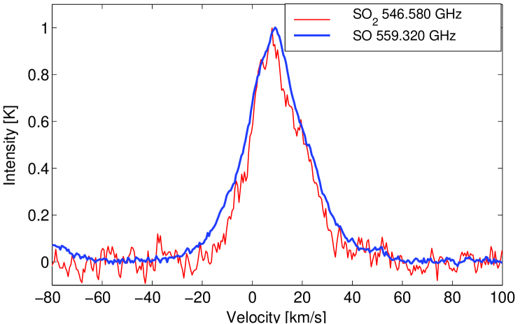
Figure 41: Comparison of the SO and SO₂ line profiles. Both lines are normalised to unity.

Sulphur-bearing species are considered to be tracers of massive outflows from a newly formed star. The high temperatures caused by the intense radiation from the driving source, or by shocks, can enhance the production of SO₂, SO and SiO. The line profile of the outflow shows a characteristic triangular line shape with broad wings as seen in examples of SO in Fig. 27, SiO in Fig. 28, SO₂ in Fig. 29, and in a comparison of SO₂ and SO in Fig. 41 (on-line material). The Orion outflows are also traced by other molecules like H₂O and CO: see Sect. 5 and 6, where also comparisons of H${}_{2}^{18}$O, SO and SO₂ are shown.

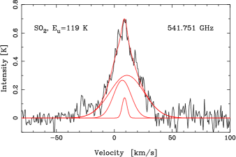
Figure 1: The $14_{3,11}$ – $13_{2,12}$ SO₂ transition with a three-component Gaussian fit shown together with the individual Gaussians. The line widths are 5 km s^-1, 18 km s^-1 and 35 km s^-1 from the CR, LVF and HVF, respectively.

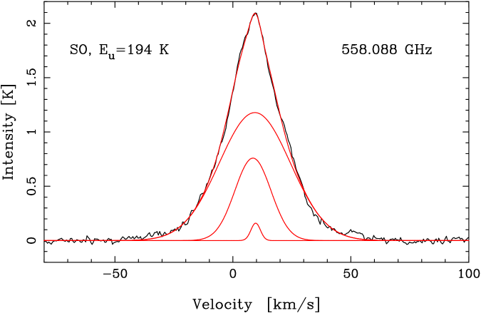
Figure 2: The $13_{12}$ – $12_{11}$ SO transition with a three-component Gaussian fit shown together with the individual Gaussians. The line widths are 5 km s^-1, 18 km s^-1 and 35 km s^-1 from the CR, LVF and HVF, respectively.

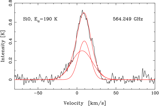
Figure 3: The $J$ = 13 – 12 SiO transition with a two-component Gaussian fit shown together with the individual Gaussians. The line widths are 18 km s^-1 and 31 km s^-1 from the LVF and HVF, respectively.

4.1.1 Sulphur dioxide (SO₂/ ³⁴SO₂)

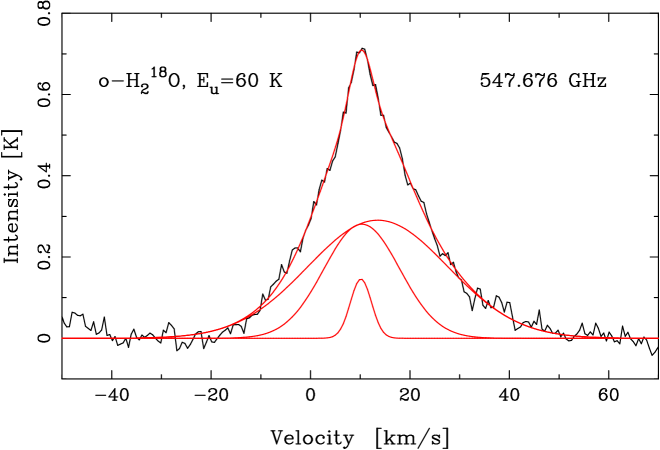
Figure 36: A three-component Gaussian fit to H${}_{2}^{18}$O shown together with the individual Gaussians. The line widths are 5 km s^-1, 18 km s^-1, and 33 km s^-1 from the CR, LVF and HVF, respectively.

We have observed 42 SO₂, and five ³⁴SO₂ transitions. Typical line profiles are shown in Fig. 29 (on-line material) with different upper state energies. As proposed by Johansson et al. (Johansson84 (1984)) the complicated SO₂ and isotopologue line shapes suggest the presence of at least two velocity components, even though the emission primarily occurs in the outflow. Figure 1 shows a three-component Gaussian fit of a typical SO₂ line with line widths of $\sim$5 km s^-1, 18 km s^-1 and 35 km s^-1 from the CR, LVF and HVF, respectively. This is very similar to the Gaussian components of SO (Fig. 2), SiO (Fig. 3), and H${}_{2}^{18}$O (Fig. 36).

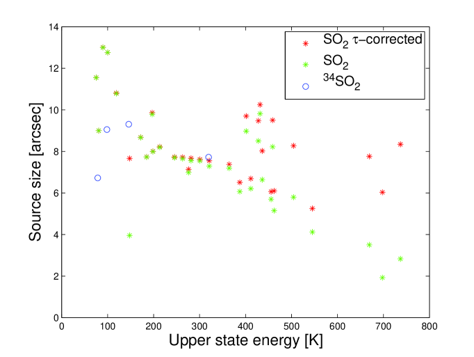
Figure 42: Source sizes for opacity-corrected SO₂ (calculated with $T_{\mathrm{ROT}}$ = 103 K and source size = 8$\arcsec$) vs. non corrected SO₂ together with ³⁴SO₂ (calculated with $T_{\mathrm{ROT}}$ = 125 K).

Figure 42 (on-line material) shows the size of the SO₂ emitting region vs. energy for each transition (Eq. 12). The mean size is found to be 8$\arcsec$, which is consistent with the aperture synthesis mapping of Wright et al. (Wright (1996)). This size is used for beam-filling corrections.

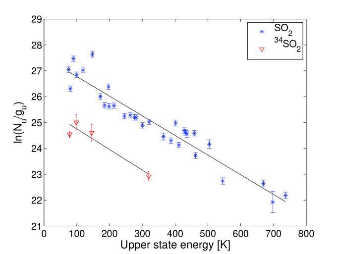
Figure 43: Rotation diagram for SO₂, not corrected for opacity, produces $T_{\mathrm{ROT}}$ = 132 K and $N_{\mathrm{ROT}}$ = 3.9$\times 10^{17}$ cm^-2 (extended source). The ³⁴SO₂ fit give $T_{\mathrm{ROT}}$ = 125 K and $N_{\mathrm{ROT}}$ = 5.4$\times 10^{16}$ cm^-2.

The high line density and the broadness of the SO₂ lines result in blends between the numerous transitions as well as with other species. There are 31 SO₂ transitions and four ³⁴SO₂ transitions without blends, which are used in a rotation diagram shown in Fig. 43 (on-line material) producing $N_{\mathrm{ROT}}$ = (3.9$\pm$0.6)$\times 10^{17}$ cm^-2, $T_{\mathrm{ROT}}$ = (132$\pm$8) K and $N_{\mathrm{ROT}}$ = (5.4$\pm$2.0)$\times 10^{16}$ cm^-2, $T_{\mathrm{ROT}}$ = 125$\pm$30 K for SO₂ and ³⁴SO₂, respectively.

However, almost all of the SO₂ transitions are optically thick which lowers the SO₂ column density. The opacity is calculated using the same excitation temperature for all transitions and the column density obtained from the ³⁴SO₂ rotation diagram (using an isotope ratio of 22.5, Table 6) and is found to be around 2 – 4 for most transitions. The opacity corrected rotation diagram is shown in Fig. 4 together with ³⁴SO₂. The column density $N_{\mathrm{ROT}}^{\tau-corr}$ increases to (1.5$\pm$0.2)$\times 10^{18}$ cm^-2 and the temperature is lowered to 103$\pm$3 K.

The isotopologue ³⁴SO₂ is optically thin, hence no opacity correction is needed. But since the lines are weak and only four, the temperature from SO₂ is applied to the rotation diagram, which increases the ³⁴SO₂ column slightly to 6.5$\times 10^{16}$ cm^-2.

As a consistency check we also use Eq. (2) together with the single optically thin SO₂ line. This $16_{\,3,13}$ – $16_{\,0,16}$ transition has an upper state energy of 148 K, and $\tau\sim 0.2$. The column density $N_{\mathrm{LTE}}$ obtained is 1.4$\times 10^{18}$ cm^-2, in agreement with $N_{\mathrm{ROT}}^{\tau-corr}$ and $N_{\mathrm{ISO}}$ from ³⁴SO₂.

Our column densities of both isotopologues are much larger than in the comparison surveys. This can partly be caused by our beam-filling correction with a rather small size, and the non-correction for opacity in W03 and S01. However, Johansson et al. (Johansson84 (1984)) and Serabyn & Weisstein (Serabyn and Weisstein (1995)) obtain a column density of about 1$\times 10^{18}$ cm^-2 (corrected for our source size) in agreement with our value.

Column densities for each subregion are estimated from the Gaussian components shown in Fig. 1 (Table 1). The rarer isotopologues are too weak for a Gaussian decomposition so opacities cannot be calculated by comparison with isotopologues. Still, the components are likely to be optically thick and therefore the sizes of the emitting regions are calculated with $T$ = 115 K for the CR, and $T$ = 103 K for the LVF and HVF. The source sizes are found to be 5$\arcsec$ for the CR and 8$\arcsec$ for both the LVF and HVF. These sizes correspond to optical depths of about 2 – 3. The opacity-corrected column densities become 2$\times$10¹⁷ cm^-2, 6$\times$10¹⁷ cm^-2, and 9$\times$10¹⁷ cm^-2 for the CR, LVF and HVF, respectively.

The elemental isotopic ratio of [³²S/³⁴S] can be estimated from a comparison of the optically thin column densities. In this way we obtain an isotopic ratio of 23$\pm$7, in agreement with most other comparison studies listed in Table 6.

As expected, no vibrationally excited lines were found. The $5_{5,1}$ – $4_{4,0}$ $v_{2}$ bending mode transition has the lowest upper state energy (822 K) of all $v_{2}$ lines in our spectral range. The calculated expected peak temperature of this line is 34 mK, with an expected line width of 23 km s^-1. Such weak and broad lines are marginally below our detection limit.

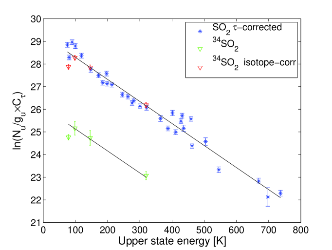
Figure 4: Rotation diagram for SO₂ produces $T_{\mathrm{ROT}}$ = 103 K (extended source). The ³⁴SO₂ fit uses the SO₂ rotation temperature.

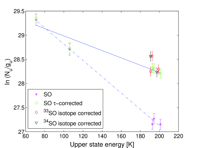
Figure 5: Rotation diagram for SO and isotopologues (extended source). The isotopologues are plotted multiplied by respective isotopic ratio. Two fits are made: the first (dashed-dotted line) is not opacity corrected ($T_{\mathrm{ROT}}$ = 59 K), while the second (solid line) is corrected for opacity ($T_{\mathrm{ROT}}$ = 132 K).

4.1.2 Sulphur monoxide (SO/³³SO/³⁴SO)

Typical line profiles are shown in Fig. 27 (on-line material). The line profiles of the high energy transitions show an even broader outflow emission, and with more pronounced high velocity line wings than does SO₂ (comparison in Fig. 41 in the on-line material). As for SO₂, the emission is primarily from the Plateau, and Friberg (Friberg84 (1984)) has shown the bipolar nature of the HVF component. The ratios of SO₂ and SO emission lines vs. velocity, also show a high degree of similarity between the line profiles except in the high velocity regime between $-$30 to $-$5 km s^-1. At these velocities SO has stronger emission than SO₂.

Figure 2 shows the 13₁₂ – 12₁₁ transition with a three-component Gaussian fit. The broad HVF component has a FWHM width of $\sim$35 km s^-1  at $\upsilon_{\mathrm{LSR}}$$\sim$ 9 km s^-1. The LVF component has widths of 18 km s^-1  at $\upsilon_{\mathrm{LSR}}$$\sim$8 km s^-1. In addition to the LVF and HVF components a third from the CR appears with a width of 5 km s^-1  at $\upsilon_{\mathrm{LSR}}$$\sim$ 9 – 10 km s^-1.

The most likely source size is 18$\arcsec$, calculated using the three optically thick SO lines. This is in agreement with the aperture synthesis mapping by Beuther et al. (Beuther (2005)), and Wright et al. (Wright (1996)), who find a larger source size for SO than for SO₂. The source size 18$\arcsec$ is used for beam-filling correction.

The rotation diagram in Fig. 5 (calculated with the total integrated intensity of the lines) displays our five SO lines. The rotation temperature without any corrections is (59$\pm$2 K) and the column density $N_{\mathrm{ROT}}$ is (1.5$\pm 0.2$)$\times$10¹⁷ cm^-2. However, the three higher energy lines have optical depth of $\sim$3, whereas the two low energy transitions are optically thin with $\tau\sim 0.1$ (Eq. 15). We make an optical depth correction for all five transitions and plot them again in Fig. 5 together with a new fit. Note that the correction is substantial for the high energy, optically thick lines (cf. Serabyn & Weisstein Serabyn and Weisstein (1995)). The rotation temperature obtained is higher than without corrections, 132$\pm$22 K, but the resulting column density is only slightly higher than that found without the corrections, $N_{\mathrm{ROT}}^{\tau-corr}$ = (1.6$\pm$0.5)$\times$10¹⁷ cm^-2. This is in agreement with the column density obtained from ³⁴SO, $N_{\mathrm{ISO}}$ = 1.9$\times$10¹⁷ cm^-2 (using 22.5 for [³²S/³⁴S]). The two optically thin SO transitions gives $N_{\mathrm{LTE}}$ = 1.8$\times$10¹⁷ cm^-2. The column densities for both isotopologues are calculated with the rotation temperature from SO.

The isotopologues, two ³³SO and three ³⁴SO transitions, are optically thin with opacities around 0.02 and 0.13, respectively. These transitions are plotted in Fig. 5 with the integrated intensities multiplied by appropriate isotopic ratios (5.5 for [³⁴S/³³S], Table 6). As seen in Fig. 5, the result of the isotopic ratio corrections is consistent with the optical depth corrected SO transitions.

As for SO₂ the column densities for each SO subregion are estimated from the Gaussian components shown in Fig. 2. Opacities cannot be calculated by comparison with the rarer isotopologues since they are too weak for a Gaussian decomposition. However, the components are likely to be optically thick and therefore the sizes of the emitting regions are calculated with $T$ = 115 K for the CR, $T$ = 132 K for the LVF, and $T$ = 100 K for the HVF. The source sizes of the CR, LVF and HVF are found to be 6$\arcsec$, 10$\arcsec$ and 14$\arcsec$, respectively. These sizes may be larger if the opacities are low. Combining calculations of source size, optical depths, and column densities, the sizes for the LVF and HVF increase slightly to 11$\arcsec$ and 18$\arcsec$, respectively. These sizes correspond to optical depths of about 2.5 and 1.0 for respective region. The opacity-corrected column densities become 1.7$\times$10¹⁶ cm^-2, 9.3$\times$10¹⁶ cm^-2, and 8.5$\times$10¹⁶ cm^-2 for the CR, LVF and HVF, respectively.

The elemental isotopic ratio of [³²S/³⁴S] and [³⁴S/³³S] can be estimated from comparisons of the column densities of the isotopologues and the optically thin SO transitions. We obtain isotopic ratios of 21.0$\pm$6 and 4.9, respectively in agreement with most other comparison studies listed in Table 6.

4.1.3 Silicon monoxide (SiO/²⁹SiO/³⁰SiO)

We have observed the transition $J\!=\!13\!-\!12$ for each isotopologue, and we show the SiO and ²⁹SiO transitions in Fig. 28 (on-line material). As for SO₂ and SO, the complicated line profile of SiO suggests emission from both the LVF and the bipolar HVF (present in aperture synthesis maps of Wright et al. Wright (1996)), with widths of 18 and 31 km s^-1 at $\upsilon_{\mathrm{LSR}}$ velocities of 9 and 7 km s^-1, respectively. Figure 3 shows the two-component Gaussian fit to SiO. The ²⁹SiO transition is located in the high-velocity wing of $o$-H₂O (at $\upsilon_{\mathrm{LSR}}$$\sim-$130 km s^-1). The width is 21 km s^-1 at a centre velocity of $\sim$9 km s^-1. The ³⁰SiO transition is a questionable assignment due to its narrow line width of 7.5 km s^-1.

Comparison of the peak antenna temperatures of SiO and ²⁹SiO shows that the SiO transition has an optical depth of $\sim$1.0. The source size (Eq. 12) is found to be 14$\arcsec$. This is used as beam-filling correction. Using a LVF temperature of 100 K (about the same temperature as the SO₂ rotation temperature), the total integrated intensity, and the simple LTE approximation, the opacity-corrected column density is found to be 4.0$\times$10¹⁵ cm^-2 for SiO.

The decomposition into subregions results in LVF and HVF source sizes of 8$\arcsec$ and 7$\arcsec$ with temperatures of 100 K for both sources. The rather small values are most likely due to the low opacity in these components and are therefore only lower limits. Assuming that the opacity in the LVF is about the same as for the total integrated emission, the LVF opacity-corrected source size increases to 10$\arcsec$. The opacity in the HVF is most likely less than in the LVF. As an upper limit the size is assumed to be the same as for the total integrated emission, which results in an HVF opacity of about 0.4. The sizes are consistent with Beuther et al. (Beuther (2005)). Note the similarity of the SO and SiO source sizes. In Sect. 6 the H${}_{2}^{18}$O sizes will also be shown to be similar. These source sizes are used to correct for beam-filling, and the resulting LVF and HVF opacity-corrected column densities are 3.3$\times$10¹⁵ and 1.8$\times$10¹⁵ cm^-2, respectively.

4.2 Outflow and Hot Core molecule

The Hot Core is a collection of warm ($\ga$200 K) and dense ($n\sim 10^{7}$ cm^-3) clumps of gas. The dominating species are oxygen-free, small, saturated nitrogen-bearing molecules such as CH₃CN and NH₃. Most N-bearing molecules are strong in the HC, and the oxygen-bearing molecules peak toward the CR (e.g. Blake et al. Blake (1987), hereafter B87; Caselli et al. Caselli93 (1993); Beuther et al. Beuther (2005)). CH₃OH is an exception with pronounced emissions from the HC as well as from the CR. In addition, high levels of deuterium fractionation are found here. Since the HC region probably contains one or more massive protostars it presents an ideal opportunity to study active gas-phase chemistry. And due to the high temperatures in both the HC and CR, the gas-phase chemistry will get a significant contribution of molecules from grain surface chemistry through evaporation of the icy mantles caused by the intense UV radiation from newly formed stars.

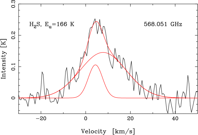
Figure 6: The H₂S 3_3,1 – 3_2,2 transition with a two-component Gaussian fit shown together with the individual Gaussians. The line widths are 8 km s^-1 and 24 km s^-1 from the HC and outflow, respectively.

4.2.1 Hydrogen sulphide (H₂S)

We observe only the 3_3,1 – 3_2,2 transition of H₂S, with emission from the HC and LVF, illustrated by a Gaussian decomposition in Fig. 6. The emission from the HC component has a width of $\sim$8 km s^-1 at $\upsilon_{\mathrm{LSR}}$$\sim$ 5 km s^-1 between velocities $-$5 to +15 km s^-1. The LVF emission has a width of $\sim$24 km s^-1 at $\upsilon_{\mathrm{LSR}}$$\sim$8 km s^-1. The line is also shown in the bottom of Fig. 25 (on-line material) together with other comparison HC molecules.

The column densities are consistent with the comparison surveys assuming typical source sizes and temperatures.

4.3 Hot Core molecules

4.3.1 Methyl cyanide (CH₃CN)

Previous observations of the high density tracer CH₃CN (e.g. Blake et al. Blake etal 86 (1986); Wilner et al. Wilner 94 (1994)) have shown that the low-$J$ transitions in the vibrational ground state appears to be a mix of CR and HC emission, while the high-$J$ transitions and all the vibrationally excited lines originate in the HC only. This is also confirmed in our survey where we observe the $30_{K}\!-\!29_{K}$ transitions with $K\!=\!0\!-\!9$, and $31_{K}\!-\!30_{K}$ with $K\!=\!0\!-\!6$ and 9. These lines suggest an origin in the HC at $\upsilon_{\mathrm{LSR}}\sim$5 – 6 km s^-1 and widths of $\sim$8 – 9 km s^-1, also consistent with W05 and C05. The 30₄ – 29₄ ground state transition is shown in Fig. 25 (on-line material). In addition we see a number of weak vibrational lines from the $v_{8}$=1 bending mode with $30_{K}\!-\!29_{K}$ where $K$ = 0 – 3. In total we observe 17 line features from this molecule. Nine of these are free from blends and are used in the rotation diagram (Fig. 7). Due to the weak lines the rotation temperature of 137$\pm$25 K and the column density of (5.0$\pm$3.6)$\times 10^{15}$ cm^-2 are comparatively uncertain. The temperature is rather low compared to W03 who estimate the temperature to 227 K, and C05 to 250 K. Still, the column density agrees well with B87, Sutton et al. (Sutton (1995), hereafter S95), W03, and C05.

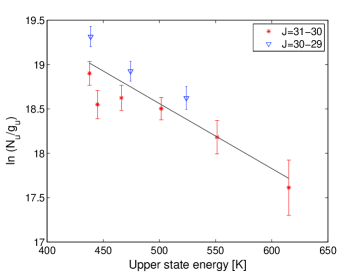
Figure 7: Rotation diagram for CH₃CN producing $T_{\mathrm{ROT}}$ = 137 K (extended source).

Wilner et al. (Wilner 94 (1994)) find an opacity of the HC emission of at most a few for the main lines. This could explain the rather low [¹³C/¹²C] ratios in Blake et al. (Blake etal 86 (1986)) and Turner (Turner 91 (1991)). Sutton et al. (Sutton 86 (1986)) suggests significant opacity from their statistical equilibrium calculations, if the HC is as small as 10$\arcsec$. This would give even higher column densities in the HC.

The partition function is calculated as recommended in Araya et al. (Araya (2005)).

4.3.2 Cyanoacetylene (HC₃N)

Two transitions of cyanoacetylene are seen, of which $J\!=\!54\!-\!53$ is a blend with CH₃OH. The transition $J\!=\!60\!-\!59$ is shown in Fig. 25 (on-line material). HC emission is here evident at $\upsilon_{\mathrm{LSR}}\sim$5 – 6 km s^-1 and a line width of $\sim$10 km s^-1. The column density is calculated with the simple LTE approximation and is in agreement with W03.

4.3.3 Carbonyl sulphide (OCS)

We have identified three transitions from carbonyl sulphide, $J\!=\!47\!-\!46$, $J\!=\!45\!-\!44$, and $J\!=\!46\!-\!45$ (shown in the on-line Fig. 25). The emission has its origin in the HC with $\upsilon_{\mathrm{LSR}}\sim$6 km s^-1, and a width of $\sim$6 km s^-1.

The estimated column density is about five times lower than found by both W03 and S95.

4.3.4 Nitric oxide (NO)

We observe three features with ${}^{2}\Pi_{3/2}$, $J$ = 11/2 – 9/2, and ${}^{2}\Pi_{1/2}$, $J$ = 11/2 – 9/2 from both e and f species, which are composed of twelve non-resolved hyperfine transitions. No separation into components is possible due to blends between the hyperfine transitions and other species. Our estimated rotation temperature from our transitions with upper state energies of 84 K and 232 K is found to be 75 K. This is highly uncertain due to the severe blends in both low energy transitions. Since S01 and C05 observed HC emission we therefore use a typical HC temperature of 200 K and source size of 10$\arcsec$. The resulting column density (using the high energy line) is in agreement with S01 and C05.

4.4 Hot Core and Compact Ridge molecules

The Compact Ridge is a more quiescent region as compared to the Hot Core. Here we find high abundances of oxygen-bearing species such as CH₃OH, (CH₃)₂O and HDO (B87; Caselli et al. Caselli93 (1993); Beuther et al. Beuther (2005)). As in the HC, the evaporation of the icy mantles in the warm CR will release molecules produced by grain surface chemistry into the gas-phase.

4.4.1 Ammonia (NH₃/¹⁵NH₃)

The symmetric top ammonia molecule is a valuable diagnostic because its complex energy level structure covers a very broad range of critical densities and temperatures (see Ho & Townes Ho and Townes (1983) for energy level diagram and review).

Many observations have been made of the NH₃ inversion lines at cm wavelengths since the first detection by Cheung et al. (Cheung68 (1968)). The upper state energy of the lowest metastable inversion lines are 24 K and 64 K comparable to 28 K for the rotational ground state transition 1₀ – 0₀ at 572 GHz. The critical density is very different though, and is 3.6$\times 10^{7}$ cm^-3 (calculated for 20 K) for the rotational ground state transition, and about 10³ cm^-3 for the inversion lines. The non-metastable inversion lines also trace higher excitation and density regions. Comparison of all these transitions could therefore give valuable information about both high- and low density and temperature regions. The previous low quantity of observations of rotational transitions is due to the fact that they fall into the submillimetre and infrared regimes, which are generally not accessible from the ground and therefore has to be observed from space.

Observations of both metastable and non-metastable inversion lines (e.g. Batrla et al. Batrla83 (1983); Hermsen et al. 1988a , 1988b ; Migenes et al. Migenes89 (1989)) have shown NH₃ in the HC, CR, ER and LVF regions. The existence of an outflow component was however questioned by Genzel et al. (Genzel82 (1982)) since the hyperfine satellite lines could cause the broadness of the line if the opacity is large.

The rotational ground state transition was first and solely detected twenty-four years ago with the Kuiper Airborne Observatory (Keene et al. Keene (1983)). Note that the Kuiper Airborne Observatory had a similar beam size (2$\arcmin$) to that of Odin (2$\arcmin.$1). Using Odin, sensitive observations have been made recently for example towards Orion KL and the Orion Bar (Larsson et al. Larsson (2003)), the $\rho$ Oph A core (Liseau et al. Liseau (2003)), Sgr B2 (Hjalmarson et al. Hjalmarson05 (2005)), as well as the molecular cloud S140. The resulting NH₃ abundance in the Orion Bar is 5$\times$10^-9 (Larsson et al. Larsson (2003)).

In this spectral survey we have observed the rotational ground state 1₀ – 0₀ transitions of NH₃ and ¹⁵NH₃, which are shown in Fig. 25 (on-line material). We show the NH₃ transition twice to emphasize the line wings. Our peak temperature agrees to within 5% with Larsson et al. (Larsson (2003)) who used a rather different Odin observational setup, demonstrating the excellent calibration of the Odin data. The vibrational transition $\nu_{2}=1$ of this line at 466 GHz has previously been observed by Schilke et al. (Schilke92 (1992)).

Fig. 8 shows our two-component Gaussian fit to the NH₃ line which has pronounced features of the CR and a broad component. The line widths are 5 and 16 km s^-1 at LSR velocities 8, and 9 km s^-1 for the CR and broad components, respectively. The CR emission was also observed by Keene et al. (Keene (1983)), while the broader component clearly seen in our Odin data, was only marginally present in their lower signal-to-noise data. Our ¹⁵NH₃ spectrum shows only evidence of the HC component (cf. Hermsen et al. Hermsen85 (1985)), with a width of $\sim$7 km s^-1 at $\upsilon_{\mathrm{LSR}}\approx 7$ km s^-1. The width of the broad NH₃ component may seem too large to have an origin in the HC. However, the broadness of the line may be caused by opacity broadening (Eq. 21; cf. Phillips et al. Phillips79 (1979)). From Eq. 16 combined with an assumed ¹⁴N/¹⁵N isotope ratio of 450 (Table 6), we estimate optical depths of $\sim$100 and $\sim$0.3 in the NH₃ and ¹⁵NH₃ HC lines, respectively. According to Eq. 21 this will broaden the

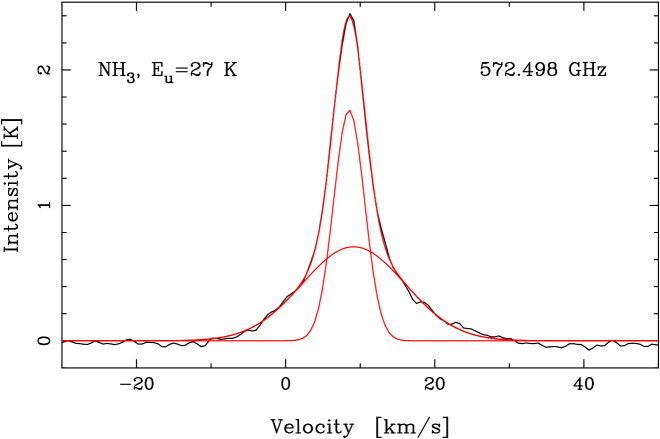
Figure 8: The NH₃ transition with a two-component Gaussian fit shown together with the individual Gaussians. The line widths are 5 km s^-1 and 16 km s^-1  from the CR and HC/outflow, respectively.

optically thick NH₃ emission line by approximately 2.6 times from a line width comparable to the optically thin ¹⁵NH₃ HC emission to a resulting width of $\sim$17 km s^-1. This is very close to the width of our Gaussian HC component, 16 km s^-1. However, the high opacity in this component will cause the line profile to be flat topped with little or no line wings. Hence our broad Gaussian component not only contains the opacity broadened HC emission but also the outflow component seen by e.g. Wilson et al. (Wilson 1979 (1979)) and Pauls et al. (Pauls 1983 (1983)), in our spectrum visible as pronounced line wings. Alternatively it could be that the HC emission is hidden by optically thick NH₃ LVF emission just as in case of water (cf. Section 6.2.2).

The NH₃ source sizes of the CR and HC regions are found to be 17$\arcsec$ and 8$\arcsec$, respectively, and are used as beam-filling corrections. The rather large CR size as compared to the 6$\arcsec$ mean source size obtained for CH₃OH, might be due to the low upper state energy of 27 K for NH₃. Figure 12 shows the decreasing methanol source size with upper state energy, where the lowest methanol transitions with upper state energies of 40 – 100 K reach a source size of $\sim$11$\arcsec$. Hermsen et al. (1988b ) find source sizes of 15$\arcsec$ and 6$\arcsec$ for the CR and HC, respectively, in agreement with our calculations. VLA maps by Migenes et al. (Migenes89 (1989)) also show that the HC emission is clumped on 1$\arcsec$ scales.

Hermsen et al. (1988b ) find a HC temperature of 160$\pm$25 K and a CR temperature above 100 K. In addition Wilson et al. (Wilson (2000)) detect an even hotter HC component with a temperature of about 400 K. Using HC and CR temperatures of 200 K and 115 K, respectively, we find a NH₃ HC column density (calculated from the optically thin ¹⁵NH₃ line) of 1.6$\times 10^{18}$ cm^-2. Our comparison surveys have no observations of this molecule, but our result agrees with Genzel et al. (Genzel82 (1982)), who report column densities of NH₃ that reach 5$\times 10^{18}$ cm^-2 from the HC, with size 10$\arcsec$ and temperatures about 200 K. Their observations also confirmed increasing line width with increasing optical depth. Hermsen et al. (1988b ) and Pauls et al. (Pauls 1983 (1983)) find values of 1$\times 10^{18}$ cm^-2 for the HC.

The optically thick NH₃ CR column density is found to be 3.4$\times 10^{15}$ cm^-2. Optical depth broadening is used to estimate the opacity in this component. Batrla et al. (Batrla83 (1983)) found an intrinsic velocity width of 2.6 km s^-1  by ammonia inversion lines observations. From a comparison with the observed line width, the opacity is estimated to be about 12 in the CR component. The opacity-corrected CR column density then becomes 4.0$\times 10^{16}$ cm^-2. This is in agreement with the estimation of Hermsen et al. (1988b ) who find a column density in the range 8$\times 10^{15}$ – 8$\times 10^{16}$ cm^-2 from the metastable (6,6) inversion line.

4.4.2 Methanol (CH₃OH/¹³CH₃OH)

Methanol is an organic asymmetric top molecule with many energy levels (see energy level diagram in Nagai et al. Nagai (1979)), and behaves like two different species labelled A and E for symmetry reasons.

We have observed 76 methanol lines of which 42 are from the $v_{t}$=1 state, which is the first excited vibrational state of the torsional motion of the CH₃ group relative to the OH group. In the on-line Fig. 32 we have collected a number of examples of typical line profiles of CH₃OH, with different upper state energies and $A$-coefficients. The rarer isotopologue ¹³CH₃OH is seen with 23 lines, of which two are vibrationally excited. Three typical line profiles are shown in the on-line Fig. 30.

The CH₃OH lines show evidence of two velocity components. One narrow, likely from the CR, with a line width of $\sim$3–4 km s^-1, and average velocity $\sim$8 km s^-1. The other broader component with a probable origin in the HC has a line width of $\sim$6 –10 km s^-1, and average velocity $\sim$7 km s^-1 (see an example of a two-component Gaussian fit in Fig. 9). This is consistent with the findings of Menten et al. (Menten (1988)), S95, C05, and also of Beuther et al. (Beuther (2005)) who locate the methanol emission to the HC as well as the CR in their SMA aperture synthesis maps. According to recent CRYRING storage ring measurements (Geppert et al. Geppert (2005); Millar Millar (2005)) the dissociative recombination of a parent ion CH₃OH${}_{2}^{+}$ + e^- $\rightarrow$ CH₃OH + H is so slow that gas-phase formation of methanol is unable to explain the abundance of this molecule, even in dark clouds where it is rare. Instead we have to rely on efficient hydrogenation reactions on grain surfaces, and subsequent release of the methanol into gas-phase. In this scenario the presence of very large amounts of CH₃OH in the compact, heated CR and HC sources is indeed expected.

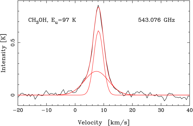
Figure 9: Methanol line with a two-component fit shown together with the individual Gaussians. The line widths are 4 km s^-1 and 10 km s^-1  from the CR and HC, respectively.

The isotopologue ¹³CH₃OH show only evidence of the narrow component, which can be well fitted by a single Gaussian with $\Delta\upsilon\approx 3$ km s^-1 at $\upsilon_{\mathrm{LSR}}\approx 8$ km s^-1. This is also consistent with Menten et al. (Menten (1988)) and Beuther et al. (Beuther (2005)). The slight broadening of the CH₃OH narrow components compared with that of ¹³CH₃OH might be caused by optical depth broadening. The ¹³CH₃OH from the HC is expected to be well below our detection limit. There are 14 ¹³CH₃OH lines free from blends with an upper state energy range between 37 – 225 K, which are used in a rotation diagram (Fig. 10). No corrections for optical depths are needed since the ¹³CH₃OH transitions are optically thin. The rotation temperature is found to be 115$\pm$16 K, and the column density (5.9$\pm$1.5)$\times 10^{16}$ cm^-2.

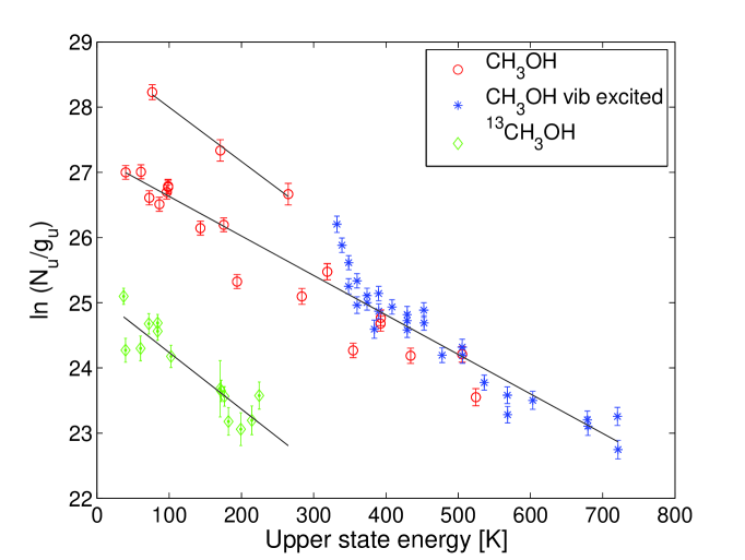
Figure 44: Rotation diagrams: CH₃OH producing $T_{\mathrm{ROT}}$ = 165 K and $N_{\mathrm{ROT}}$ = 9.3$\times 10^{17}$ cm^-2 (not opacity corrected); three optically thin CH₃OH lines produces $T_{\mathrm{ROT}}$ = 120 K and $N_{\mathrm{ROT}}$ = 2.6$\times 10^{18}$ cm^-2;

If we exclude blended and very weak lines we have 50 CH₃OH lines with an upper state energy range from 40 to 721 K. The large number of lines and the wide temperature range make methanol well suited to be used in a rotational diagram. However, one difficulty that may occur with this method is that the optical depths may vary considerably between the CH₃OH transitions. In the rotation diagram seen in Fig. 44 (on-line material) the lines are plotted (using the total integrated intensity) without any attempt to correct for optical depth or beam-dilution. As can be seen there is a large scatter of the CH₃OH lines. Three transitions with upper state energies of 77, 171 and 265 K lie clearly very high above the others due to their low transition probability and low opacity. A separate fit of these three lines is made and the resulting beam-filling corrected column density becomes (2.6$\pm$0.4)$\times 10^{18}$ cm^-2. This is about 3 times higher than the resulting column density from all the lines, (9.3$\pm$1.1)$\times 10^{17}$ cm^-2. This indicates that opacity correction needs to be included in the rotation diagram.

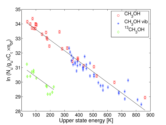
Figure 45: CH₃OH forward model producing $T_{\mathrm{ROT}}$ = 136${}^{+3}_{-4}$ K, $N$ = (1.3$\pm$0.1)$\times 10^{18}$ cm^-2 and a source size of 6$\arcsec^{+0.1}_{-0.3}$. The ¹³CH₃OH forward model use the rotation temperature and source size obtained from CH₃OH.

Using the forward model, which includes opacity and beam-filling correction (see Fig. 45 in the on-line material), we find a column density of (1.3$\pm$0.1)$\times 10^{18}$ cm^-2 in a source size of 6″. (This size is used as beam-filling correction in all calculations of the column densities above.) The scatter in the rotation diagram is reduced and approaches the column density obtained from the three (assumed) optically thin lines. However, since this method has a tendency to underestimate the column density we proceed with opacity correction of the traditional rotation diagram. We note that most of the low energy lines seem to be optically thick (opacities between $\sim$1 – 6) and most of the high energy lines seem to be optically thin (opacities between $\sim$0.3 – 1.5). The rotation temperature would be too high if not opacity corrected.

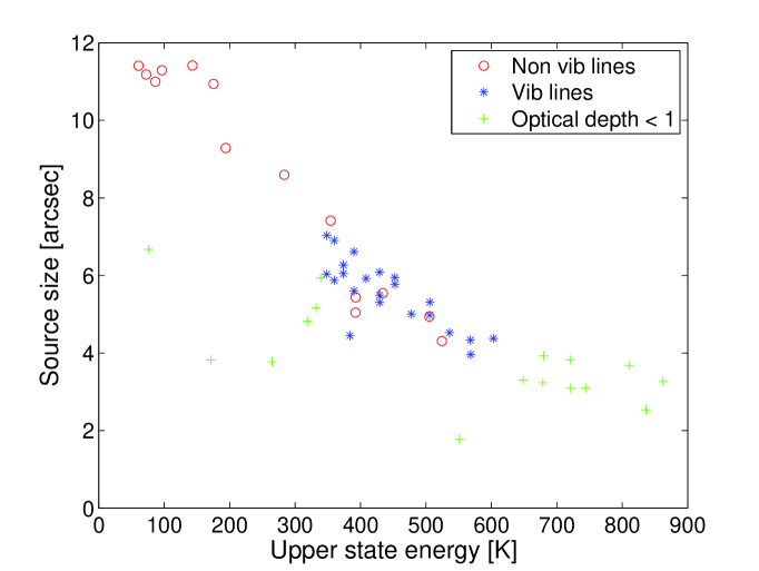
Figure 46: Source size variation with energy for CH₃OH (no opacity corrections). The low-energy transitions have larger source sizes than higher-energy transitions. Note that all lines with an optical depth less than one, fall below the general trend of decreasing source size with higher energy, since Eq. (14) is only valid for optically thick lines.

An additional complication is that the extent of the emitting regions may be different for lines of different energy (cf. Menten et al. Menten86 (1986)). This is affecting our estimation of the opacity since we need a total column density (corrected for beam-filling) in the calculations. The on-line Fig. 46 shows that the source size of the low-energy lines varies between 5 – 12$\arcsec$, whereas the size of the high-energy lines is almost constant (about 6$\arcsec$), based on Eq. (14) at $T_{\mathrm{ROT}}$ = 120 K.

In Fig. 10 we show the opacity corrected rotation diagram. The opacity is calculated using the column density obtained from the three optically thin lines corrected for different beam-fillings for each transition, and the same excitation temperature for all lines (120 K). The scatter in the plot is even more reduced than in the forward model and the resulting column density becomes (3.4$\pm$0.2)$\times 10^{18}$ cm^-2. This is much higher than in our comparison surveys, but consistent with Johansson et al. (Johansson84 (1984)), Menten et al. (Menten86 (1986)), and S01 using the ¹³CH₃OH column density (all corrected for our source size).

The rotation temperature is 116$\pm$2 K with opacity correction which is the same as produced by the ¹³CH₃OH rotation diagram (115$\pm$16 K) and the optically thin fit (120$\pm$10 K). The forward model produces a slightly higher temperature (136$\pm$4 K), which suggests that the opacity correction is too low with this method.

There is also a possibility that the high- and low energy lines are emitted from different regions even though our rotation diagram does not indicate a change of rotation temperature. Using the Gaussian decomposition of the 27 strongest lines, we note that the integrated intensity of the low energy lines is dominated by the narrow CR component, and the high energy lines by the broad HC emission.

When calculating the opacity of the components we again take into account the varying source size with energy. However, Fig. 12 shows that the pronounced variation in size is only true for the narrow component. The broad component seems to have approximately the same size as the energy increases. This again supports the scenario in which the narrow component arises in the CR, which is denser and hotter in the central parts. Hence only the central parts have the ability to emit the high energy lines. The broad component keeps the small size across the transition energy range, supporting an origin in the HC. This source is small and hot and thus can emit all transitions throughout the whole region. The opacity of the CR component is found to be higher than in the HC component which is about 1 or less.

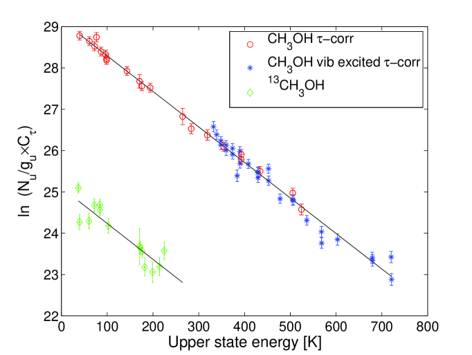
Figure 10: CH₃OH opacity corrected rotation diagram producing $T_{\mathrm{ROT}}$ = 116 K (extended source). The opacity is calculated with varying source-sizes with energy. The ¹³CH₃OH rotation diagram gives a temperature of 115 K.

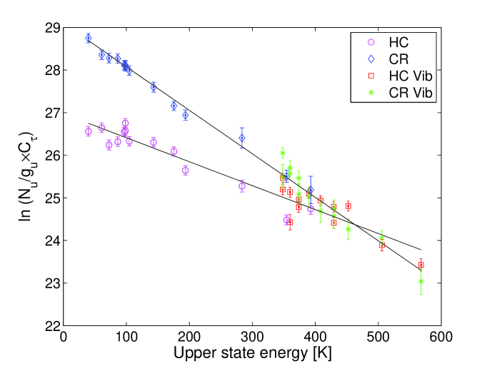
Figure 11: Two component CH₃OH opacity corrected rotation diagram producing $T_{\mathrm{ROT}}$ = 178 K and 98 K for the HC and CR, respectively (extended source). The opacity is calculated with the same parameters together with varying source-size with energy.

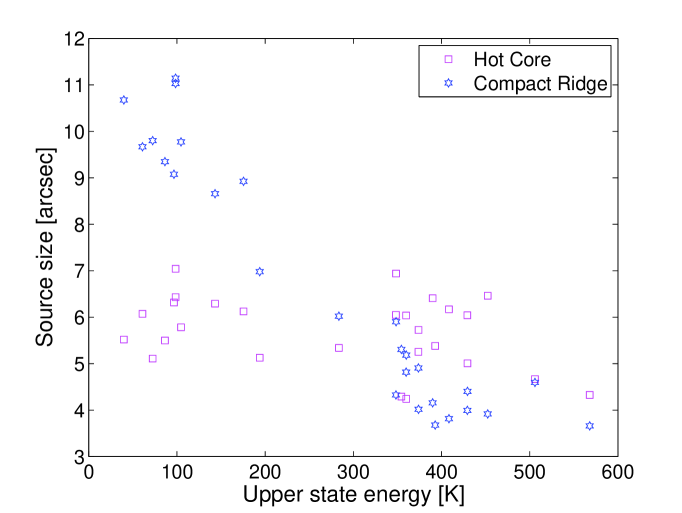
Figure 12: Source size variation with energy for the CR and HC components of CH₃OH (opacity-corrected with $N_{\mathrm{CR}}$ = 1.7$\times 10^{18}$ cm^-2, $T_{\mathrm{CR}}$ = 120 K and $N_{\mathrm{HC}}$ = 7.9$\times 10^{17}$ cm^-2, $T_{\mathrm{HC}}$ = 200 K )

.

Plotting the components in a opacity corrected rotation diagram (Fig. 11), produces column densities and rotation temperatures for each region: $N_{\mathrm{ROT}}$ = (2.4$\pm$0.2)$\times 10^{18}$ cm^-2, $T_{\mathrm{ROT}}$ = 98$\pm$2 K and (7.9$\pm$1.0)$\times 10^{17}$ cm^-2, $T_{\mathrm{ROT}}$ = 178$\pm$11 K for the CR and HC, respectively. Both column densities are much higher than in our comparison surveys, but agrees well with S95 (corrected for our source size). The calculated temperatures are lower than in the comparison surveys, but the high apparent rotation temperatures may be caused by high opacity. Hollis et al. (Hollis 83 (1983)) found that the ground-state transitions originate in a 90 K region, while the torsionally excited transitions come from a 200 K region.

The isotopic ratio of ¹²C/¹³C can be estimated from the ratio of the optically thin CH₃OH and ¹³CH₃OH column densities, and is found to be 57$\pm$14. This is consistent with previous estimates (Table 6).

4.5 Compact Ridge molecules

4.5.1 Dimethyl ether ((CH₃)₂O)

This molecule is affected by two internal rotors which are the origin of the fine structure lines of the AA, AE, EE and EA symmetries (Groner et al. Groner98 (1998)). The emission only shows characteristics of the CR with narrow widths of 3 – 4 km s^-1 at $\upsilon_{\mathrm{LSR}}$ velocities of $\sim$6 – 8 km s^-1.

Since we cannot resolve these fine structure transitions, we treat them as one single line. The statistical weights and the partition function are changed accordingly. We observe 47 quartets out of which 37 are free from blends and hence can be used in the rotation diagram shown in Fig. 13. The resulting beam-filling corrected column density is (1.3$\pm$0.3)$\times$$10^{17}$ cm^-2 and the rotation temperature is 112$\pm$8 K, which is higher than in the comparison line surveys (Table 1). The adopted source size is the same as obtained for CH₃OH, since these molecules most likely have a rather similar origin in the CR. This is also verified when calculating the source size with Eq. 14, assuming an opacity larger than unity. For a temperature of 112 K we find a CR size of 5 – 6$\arcsec$. This is also indicating optically thick lines which could increase the column density even further.

4.5.2 Thio-formaldehyde (H₂CS)

Five transitions of the CR-emitting H₂CS are observed, of which the 16_3,13 – 15_3,12 transition is a blend with a U-line. The line profile of the 14_1,13 – 13_1,12 transition is shown in Fig. 33 (on-line material). The four lines with no blends are used in the rotation diagram shown in Fig. 14, producing a rotation temperature, very similar to that of CH₃OH, $T_{\mathrm{ROT}}$ = (93$\pm$4) K. The resulting beam-filling corrected column density is (1.3$\pm$0.2)$\times$$10^{15}$ cm^-2, with a source size of 14$\arcsec$ guided by our calculations for the H₂CO optically thick CR emission (see Sect. 4.6.1).

A comparison of the H₂CS and the optically thin H${}_{2}^{13}$CO results in a molecular abundance ratio of H₂CO/H₂CS$\sim$15. This is lower than the quoted [O/S] ratio of 35 (on-line Table 6) from Grevesse et al. (Grevesse (1996)). From the comparison of H₂O and H₂S in Sect. 6 we obtain a similar value of $\sim$20.

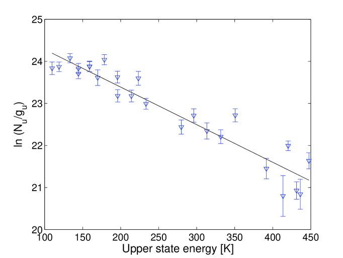
Figure 13: Rotation diagram for (CH₃)₂O producing $T_{\mathrm{ROT}}$ = 112 K (extended source).

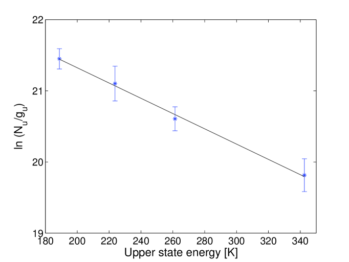
Figure 14: Rotation diagram for H₂CS producing $T_{\mathrm{ROT}}$ = 93 K (extended source).

4.5.3 Thioformyl cation (HCS⁺)

The thioformyl cation previously has not been seen either by W03 nor S01, and here we only observe the $J\!=\!13\!-\!12$ transition as a visible blend with ³³SO. Due to the blend we cannot analyse this transition further, but this emission is most likely emitted in the same small hot and dense CR source as CH₃OH and (CH₃)₂O.

4.6 Outflow and Compact Ridge molecule

4.6.1 Formaldehyde (H₂CO/H${}_{2}^{13}$CO/HDCO)

We detect three transitions from each of H₂CO and HDCO, and one transition from H${}_{2}^{13}$CO. Since the energy range is small (106 – 133 K), no rotation diagram can be made. The 8_1,8 – 7_1,7 transition of H₂CO is shown in Fig. 33 (on-line material), together with the same transition of H${}_{2}^{13}$CO and the 9_1,9 – 8_1,8 transition of HDCO. The H₂CO 8_0,8 – 7_0,7 transition shows a blend with Hot Core NS at 576.720 GHz. The 8_1,7 – 7_1,6 transition of H₂C¹⁸O is tentatively found at 571.477 GHz.

The H₂CO lines show two velocity components. Figure 15 shows a two-component Gaussian fit. The narrow component from the CR has widths of $\sim$5 km s^-1 at $\upsilon_{\mathrm{LSR}}\sim$8.5 km s^-1, and the broader component from the LVF has widths of $\sim$19 km s^-1 at $\upsilon_{\mathrm{LSR}}\sim$8 km s^-1. H${}_{2}^{13}$CO and HDCO show only emission from the CR with similar widths and LSR velocities as for the narrow H₂CO component. Comparison of the CR component of the H₂CO 8_1,8 – 7_1,7 transition with the same H${}_{2}^{13}$CO transition, results in optical depths of $\sim$6.6 and $\sim$0.1, respectively (using [¹²C/¹³C] = 60).

Since the CR component is optically thick in H₂CO, this source size is calculated with Eq. 14 and is found to be as large as 14$\arcsec$ for a temperature of 115 K, in agreement with Mangum et al. (Mangum90 (1990)). The LVF source size becomes 10$\arcsec$, which might be caused by a low opacity. Hence a LVF size of 15$\arcsec$ is used for beam-filling correction. The resulting CR and LVF column densities are 3.0$\times$10¹⁵ cm^-2 and 4.3$\times$10¹⁵ cm^-2, respectively. With the use of the optically thin H${}_{2}^{13}$CO the CR column density increases to 2.0$\times$10¹⁶ cm^-2, in agreement with Turner (Turner90 (1990)), Mangum et al. (Mangum90 (1990)), and S95.

Since H₂CO is optically thick we cannot calculate the [¹²C/¹³C] elemental ratio. But with the use of the optically thin H${}_{2}^{13}$CO and HDCO, the abundance ratio of D/H is estimated to $\sim$0.01, which implies a high deuterium fractionation in the CR. Turner (Turner90 (1990)) derived a ratio of HDCO/H₂CO = 0.14${}^{+0.12}_{-0.07}$ and D₂CO/HDCO = 2.1${}^{+1.2}_{-0.5}$$\times$10^-2 for the CR. These large abundance ratios were interpreted as a result of active grain surface chemistry.

4.7 Outflow, Hot Core and Compact/Extended Ridge molecules

4.7.1 Carbon monosulfide (CS/¹³CS)

Fig. 16 shows a three-component Gaussian fit to the observed $J$ = 10 – 9 transition of CS. Emission is seen from a narrow component, the HC and the LVF at LSR velocities 9, 7 and 10 km s^-1 with widths 4, 9 and 18 km s^-1, respectively. The narrow component may have an origin either from the ER or the CR, hence the column density is calculated with both alternatives. The CS line is also compared to H₂CS and isotopologues of H₂CO in Fig. 33 (on-line material).

The ¹³CS $J\!=\!12\!-\!11$ transition is observed with emission from a narrow (ER or CR) component, but is blended with a ³⁴SO₂ transition. This makes the Gaussian fit with a width of 5 km s^-1, at LSR velocity 7 km s^-1 approximate. Comparison of peak antenna temperatures of the isotopologues (using a ¹²C/¹³C ratio of 60) suggests that the narrow CS component is optically thick ($\tau\sim 6-12$). The source size of an ER component is calculated with Eq. 14 and is found to be 30$\arcsec$ for at temperature of 60 K. This suggests that either the emission of this component is rather extended and clumpy (see Sect. 8), or has an origin in the CR. For a typical CR temperature of 115 K, we find a size of 20$\arcsec$.

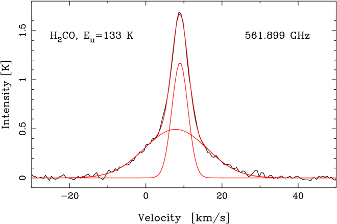
Figure 15: The H₂CO 8_1,8 – 7_1,7 transition with a two-component Gaussian fit shown together with the individual Gaussians. The line widths are 5 km s^-1 and 19 km s^-1 from the CR and LVF, respectively.

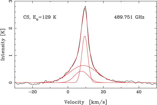
Figure 16: The CS $J$ = 10 – 9 transition with a three-component Gaussian fit shown together with the individual Gaussians. The line widths are 4 km s^-1, 9 km s^-1, and 18 km s^-1  from the CR/ER, the HC and LVF, respectively.

The resulting column densities are listed in Table 1. The column density of the LVF agrees well with B87, S95, S01 and C05, and the HC column also agrees with S95, but is lower than found in C05. The narrow component from either the CR och ER is more difficult to compare. Our ER column agrees rather well with B87, but is an order of magnitude lower than found by S95. As CR emission it agrees with S95. The differences may arise due to opacity, beam-sizes and energy levels.

4.7.2 Hydrogen isocyanide (HNC)

Figure 17 shows a four-component Gaussian fit of the HNC $J\!=\!6\!-\!5$ transition with an upper state energy of 91 K, and a U-line seen in the red-ward LVF line wing at a velocity of 22 km s^-1. As for CS, three velocity components, from the ER, HC, and LVF, are clearly seen at $\upsilon_{\mathrm{LSR}}$= 9, 6 and 7 with widths of 4, 9 and 27 km s^-1, respectively. The sizes and temperatures for the subregions are taken to be representative of typical values (see Table 1). The HNC line is also shown in Fig. 31 (on-line material).

4.8 PDR/Extended Ridge and Hot Core molecule

4.8.1 The cyanide radical (CN)

The main CN emission has its origin in the PDR/ER region and the HC (Rodríguez-Franco et al. Rodriguez-Franco (1998)) at $\upsilon_{\mathrm{LSR}}\sim 9$ and 8.5 km s^-1 with widths of $\sim$4 and $\sim$10 km s^-1, respectively. In total we have observed three lines with 8 non-resolved hyperfine structure features. Figure 31 (on-line material) shows one of the $N\!=\!5\!-\!4$ transitions, consisting of three non-resolved hyperfine structure lines, with two additional ones in the line wing at a velocity of 1 km s^-1. The same transitions are shown in Fig. 18 with a three-Gaussian fit of the five transitions. No rotation diagram is made since the upper state energy of 54 K is the same for all transitions.

Using Gaussian fits, the LTE approximation and typical temperatures and source sizes, the column densities for the HC and PDR/ER regions are estimated to be 7.9x10¹⁵ cm^-2, and 4.9x10¹³ cm^-2 for the HC and PDR/ER, respectively. Our comparison surveys have no observations of CN, but Rodríguez-Franco et al. (Rodriguez-Franco01 (2001)) obtained column densities by CN mapping, ranging from 10¹³ cm^-2 in the Trapezium region to 10¹⁴ – 10¹⁵ cm^-2 in the Ridge region. S95 find $N$ = 1$\times$10¹⁵ cm^-2 with a 14$\arcsec$ beam, and B87 also find the same CN column density with a 30$\arcsec$ beam.

4.9 Extended Ridge molecule

4.9.1 Diazenylium (N₂H⁺)

The diazenylium transition $J\!=\!6\!-\!5$ is shown in Fig. 31 (on-line material). The width of $\sim$5 km s^-1 at $\upsilon_{\mathrm{LSR}}\approx 9$ kms^-1 indicates an ER origin of the emission, in agreement with mapping of the $J$ = 1 – 0 transitions by Womack et al. (Womack90 (1990)) and Ungerechts et al. (Ungerechts97 (1997)). The column density of 1.0$\times$10¹² cm^-2, that we calculate using the simple LTE approximation, is much lower than that found by Ungerechts et al. (Ungerechts97 (1997)), 8.4$\times$10¹² cm^-2.

4.10 Unidentified line features

We observe 64 unidentified line features. Tentative assignments have been given to 26 lines, such as the first tentative detections of ND, and of the anion SH^- (see Fig. 34, Tables 34, and 35 in the on-line Material and Table 3 in Paper I). There are 28 U-lines, i.e. clearly detected lines, and 36 T-lines, which means that they are only marginally visible against the noise or in a blend. The tentative assignments also include the species SO⁺, CH₃CHO, CH₃OCHO, SiS, HNCO, H₂C¹⁸O, and a high energy HDO line. For details see Paper I.

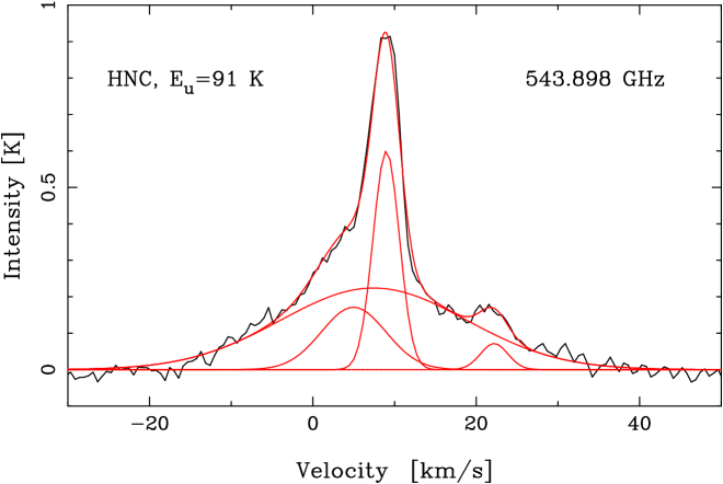
Figure 17: The HNC $J$ = 6 – 5 transition and a U-line at 543.873 GHz with a four-component Gaussian fit shown together with the individual Gaussians. The line widths are 4 km s^-1 for the U-line, 4 km s^-1, 9 km s^-1, and 27 km s^-1for the HNC ER, HC and outflow components, respectively.

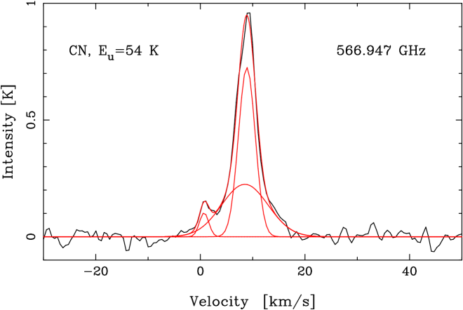
Figure 18: CN with a three-component Gaussian fit of five unresolved hyperfine-structure lines shown together with the individual Gaussians. The widths are 4 km s^-1 and 11 km s^-1 for the PDR/ER and HC components of the three strong hyperfine-structure lines, respectively, and 2 km s^-1 for the weak transitions at a velocity of 0 km s^-1.

The strongest U-line is found at 542.945 GHz with a peak intensity of 140 mK. The line appears to show emission from two components, probably the CR and the HC (see Fig. 34 in the on-line material).

5 Carbon monoxide (CO/¹³CO/C¹⁷O/C¹⁸O), carbon (C) and H₂ column densities

We have observed the $J\!=\!5\!-\!4$ transition of CO, ¹³CO, C¹⁷O, and C¹⁸O (Fig. 26). The CO line is the most intense single line in our 42 GHz wide band. The FWZP (Full Width Zero Power) of CO is approximately 230 km s^-1, as compared to 120 km s^-1 reported in Wirström et al. (Wirstrom (2006), hereafter W06), a result of our much lower noise level. Since W06 also used Odin but with another observation mode, we can again demonstrate the high accuracy of the Odin calibration with a comparison of the amplitudes, which agree within less than five percent.

As pointed out in W06 it is clear that CO $J\!=\!5\!-\!4$ has emission from at least three different components – LVF, HVF and a narrow component. The high brightness temperature of the last component suggests that this emission originates in the extended and warm PDR, whereas the narrow components from the optically thin isotopologues have approximately equal emission from the PDR and the colder ER gas behind it. We observe all three components in the CO and ¹³CO emission, but only the narrow ER/PDR component and the LVF for the C¹⁷O and C¹⁸O isotopologues (W06). The Gaussian components are given in Tables 8 and 32 in the on-line material, and agree well with W06, especially when our higher signal-to-noise ratio is taken into account, which enables us to see line wings that were previously unobserved.

A summary of the resulting column densities, estimated optical depths, used source sizes and temperatures is found in Table 2, and also in more detail in the on-line Table 8. Here also column densities calculated from all isotopologues are given together with the parameters of the Gaussian fits. Note that the column density for the CO narrow component (calculated from C¹⁷O) is lowered by a factor of two, since this component only has emission from the PDR, while the isotopologues have approximately equal emission from both the PDR and ER. For detailed arguments see W06.

The only observed atomic species in this survey is the ${}^{3}P_{1}$ – ${}^{3}P_{0}$ transition of C at 492.1607 GHz. It shows a narrow line profile from an extended emission with a width of 4.5 km s^-1, at LSR velocity $\sim$9 km s^-1. Due to the loss of orbits during this observation, the noise level here is 200 mK, as compared to our average level of 25 mK in the rest of the spectral survey. This makes it impossible to distinguish a possible broad emission in this transition. Our beam-averaged column density of C is 5.6$\times$$10^{17}$ cm^-2. Tauber et al. (Tauber (1995)) find a lower limit for a beam-averaged C column density of $\sim$7$\times$$10^{17}$ cm^-2  (beam size 17$\arcsec$) in the Orion bar. Ikeda et al. (Ikeda (1999)) find a column density very similar to ours (6.2$\times$$10^{17}$ cm^-2) from observations of the 492.1607 GHz transition with the Mount Fuji submillimetre-wave telescope towards the Orion KL position, in a HPBW of 2$\arcmin$.2. The optical depth was estimated to be 0.2. B87 find $N\ga$7.5$\times$$10^{17}$ cm^-2 with a 30$\arcsec$ beam towards the Orion KL region. Plume et al. (Plume (2000)) presented maps of the same transition, obtained with the SWAS satellite, resulting in an average column density of 2$\times$$10^{17}$ cm^-2.

When estimating abundances we need comparison column densities of H₂ for each subregion (results also given in Table 2). This is provided by C¹⁷O for the PDR/ER and LVF components, using [CO]/[H₂]=8$\times$$10^{-5}$ (e.g. Wilson & Matteucci Wilson Matteucci (1992)), an isotope ratio [¹⁸O]/[¹⁷O] = 3.9 (Table 6), together with [¹⁶O]/[¹⁸O]=330 (Olofsson 2003b ). The latter value was found from high S/N S¹⁸O observations of molecular cloud cores. This is somewhat lower than the usually quoted value of 560 (Wilson & Rood Wilson and Rood (1994)), valid for the local ISM and estimated from H₂CO surveys in 1981 and 1985. A likely explanation for the lower value is a local enrichment of ¹⁸O relative to ¹⁶O by the ejecta from massive stars. For the HVF component we use ¹³CO since C¹⁷O has no HVF emission.

The resulting H₂ column density from the LVF is 3.2$\times 10^{23}$ cm^-2. This is close to the limits given by Masson et al (Masson (1987)) (3 – 10)$\times 10^{22}$ cm^-2, as well as 1$\times 10^{23}$ cm^-2 by Genzel & Stutzki (Genzel and Stutzki (1989)). Wright et al. (Wright 2000 (2000)) find a beam-averaged H₂ column density of 2.8$\times 10^{23}$ cm^-2 from observations of the 28.2 $\mu$m H₂ 0–0 S(0) line for a temperature of 130 K (beam size 20$\arcsec\times 33\arcsec$).

Our resulting HVF H₂ column density is 3.9$\times 10^{22}$ cm^-2, in agreement with the Genzel & Stutzki value of 5$\times 10^{22}$ cm^-2. In contrast, Watson et al. (Watson (1985)) found that the HVF column of warm shock heated H₂ is only 3$\times 10^{21}$ cm^-2, a result based upon their KAO observation of high-$J$ CO lines.

Tauber et al. (Tauber (1995)) reported an average H₂ column density of $\sim$3$\times 10^{22}$ cm^-2 from the Orion Bar (calculated from ¹³CO mapping). This is in agreement with our total narrow component, which we find to be 4$\times 10^{22}$ cm^-2. When we calculate the abundances in Sect. 7, we divide this value by two, since there are about equal contributions from the PDR and ER to the C¹⁷O emission (W06). Our value is also consistent with the results of Goldsmith et al. (Goldsmith97 (1997)) convolved with the 2$\arcmin$.1 Odin beam.

Figure 19: Water and isotopologues. The $o$-H${}_{2}^{17}$O is reconstructed spectra with blending lines subtracted. An intensity scale factor is given after the molecular species.

6 Water ($o$-H${}_{2}^{16}$O, $p$-H${}_{2}^{16}$O, $o$-H${}_{2}^{17}$O, $o$-H${}_{2}^{18}$O, HDO)

6.1 Correcting the water emission lines for blends

Because of the large number of methanol and sulphur dioxide lines observed, they cause the most common blends in all lines. Since we are particularly interested in water, we attempt to reconstruct the water isotopologues without blends. We use observed transitions in our survey with similar parameters ($E_{u}$, $A$-coefficient and $g_{u}$), and scale them with the parameters of the blending lines before removal from the water isotopologue line of interest. The molecular line parameters of the blending transitions are found in the on-line Tables (9, 10 and 20).

Two lines are blended with the $o$-H${}_{2}^{18}$O $1_{1,0}$ – $1_{0,1}$ ground state rotational transition. The ³⁴SO₂ $21_{3,19}$ – $20_{2,18}$ transition is blended with the red wing, and in the blue wing there is an overlapping methanol line, $15_{1,15}$ – $15_{2,14}$, $v_{t}$=1. However, since the simultaneous observations of $o$-H${}_{2}^{17}$O show that the H${}_{2}^{18}$O transition is optically thick even in the line wings (see next section), we do not attempt to remove these blending transitions.

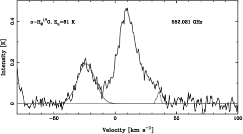
Figure 38: H${}_{2}^{17}$O before removal of blends with reconstructed lines from SO₂ and CH₃OH shown..

The $o$-H${}_{2}^{17}$O ground state rotational transition is, however, optically thin in the line wings, and we therefore remove three blending lines. In Fig. 38 (on-line material) we show two of the blending lines together with the $o$-H${}_{2}^{17}$O line. In the blue $o$-H${}_{2}^{17}$O wing the blending SO₂ transition $26_{\,6,20}$ – $26_{\,5,21}$ is overlapping. In the red wing there are two blends. One from the $6_{\,6,1}$ – $7_{5,3}$ methanol transition shown, and one from the very weak SO₂ $34_{1,33}$ – $34_{0,34}$ transition.

6.2 Water analysis

We have observed the 1_1,0 – 1_0,1 ground state rotational transition of $o$-H₂O and its isotopologues $o$-H${}_{2}^{18}$O and $o$-H${}_{2}^{17}$O, which mainly show emission from the Plateau. A very weak feature at 489.054 GHz is tentatively identified as the HC-tracing 4_2,3 – 3_3,0 transition of $o$-H${}_{2}^{18}$O with an upper state energy of 429 K. The HC-tracing $p$-H₂O transition 6_2,4 – 7_1,7 with an upper state energy of 867 K, is also observed, as well as the 2_0,2 – 1_1,1 HDO transition showing emission from the CR, HC and LVF. Figure 19 shows all detected water lines after removal of some blends in H${}_{2}^{17}$O as discussed in the previous section.

The optical depths, column densities, assumed source sizes and excitation temperatures are found in Table 2, and in more detail in Table 7 (on-line material), together with the parameters of the Gaussian fits.

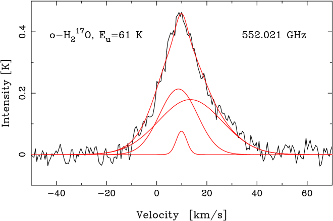
Figure 35: A three-component Gaussian fit to H${}_{2}^{17}$O shown together with the individual Gaussians. The line widths are 5 km s^-1, 18 km s^-1, and 30 km s^-1 from the CR, LVF and HVF, respectively.

Both the $o$-H${}_{2}^{18}$O and $o$-H${}_{2}^{17}$O ground state rotational transition show features of a weak, narrow component from the CR, a broad stronger component from the LVF, and with HVF emission mainly in the red wing. Figures 35 and 36 (on-line material) show three-component Gaussian fits to the water isotopologues. The emission from the ER and PDR is considered to be very low since the water mainly will be frozen onto the dust grains at the rather low temperatures in this region.

The $o$-H₂O line is very optically thick at all velocities as seen in Fig. 39 (on-line material) which displays the ratio of $o$-H₂O and $o$-H${}_{2}^{18}$O. The excitation conditions for these two isotopologues are therefore very different. A similar figure of the ratio of $o$-H${}_{2}^{18}$O and $o$-H${}_{2}^{17}$O (Fig. 40 in the on-line material) shows an almost constant ratio of 1.5 for velocities between $-$10 and +30 km s^-1. This demonstrates that the two line profiles are almost identical, and that the $o$-H${}_{2}^{18}$O emission is rather optically thick at all velocities since [¹⁸O/¹⁷O] = 3.9. By comparison of column densities from the total integrated intensities, the optical depths for $o$-H${}_{2}^{17}$O and $o$-H${}_{2}^{18}$O, are 0.9 and 3.4, respectively. The small changes of the ratio with velocity as seen in Fig. 40 also are consistent with our decomposition into Gaussian components. The LVF is optically thick in both isotopologues, whereas the HVF and CR have lower optical depths causing increase of the ratio at their emission velocities.

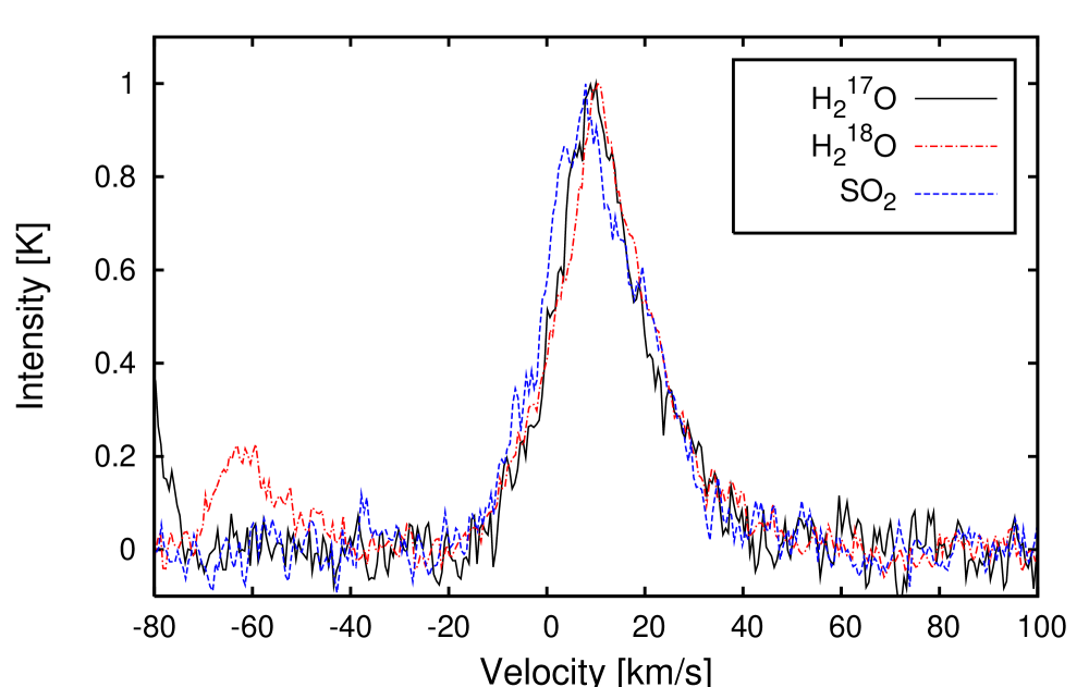
Figure 20: Comparison of H${}_{2}^{18}$O, with H${}_{2}^{17}$O, and the 19_3,17 – 18_2,16  SO₂ transition, all normalised with respective peak temperature. The high degree of similarity of all three line profiles suggests an origin in the same gas and velocity fields, mainly from the LVF with additional emission from HVF in the red wings.

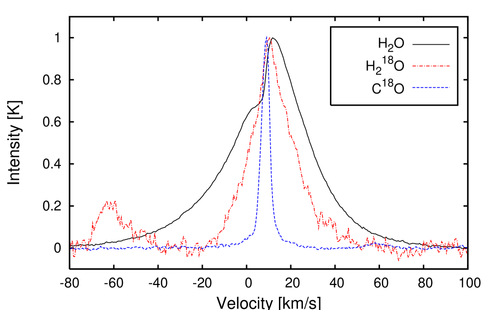
Figure 21: Comparison of the optically thick self-absorbed $o$-H₂O with $o$-H${}_{2}^{18}$O and C¹⁸O $J$ = 5 – 4, all normalised with respective peak intensity. The LVF self-absorption of $o$-H₂O in the blue wing is seen when compared to $o$-H${}_{2}^{18}$O, which shows LVF emission in both wings and HVF emission mainly in the red wing.

6.2.1 Ortho-H₂O from the Low- and High Velocity Flow and the Compact Ridge

The similarity of the line profiles is also illustrated in Fig. 20 showing a comparison of $o$-H${}_{2}^{17}$O, $o$-H${}_{2}^{18}$O and the 19_3,17 – 18_2,16 SO₂ transition, all normalised to their respective peak temperature. The remarkable similarity of the line profiles suggests a very similar origin and chemistry of the water isotopologues and SO₂: the LVF and with additional HVF emission mainly in the red wings.

The resulting column densities (found in Table 2 and in the on-line Table 7) are calculated with the simple LTE approximation and for an $ortho/para$ ratio of 3. As a first approximation of the column density we have used the full integrated intensity of the lines, assuming the Plateau to be the main emitting source (with $T_{\mathrm{ex}}$ = 72 K and a source size of 15$\arcsec$, see below). We have also calculated the column densities for the different subregions using the Gaussian components. In addition, the $o$-H${}_{2}^{17}$O and $o$-H${}_{2}^{18}$O column densities are calculated with and without optical depth corrections. Since the $o$-H₂O transition is highly optically thick, we calculate the column density from $o$-H${}_{2}^{17}$O and $o$-H${}_{2}^{18}$O. With isotope ratios of [¹⁸O]/[¹⁷O]=3.9 and [¹⁶O]/[¹⁸O]=330 (Table 6), we determine the opacity-corrected column density of H₂O to be 1.7$\times 10^{18}$ cm^-2. The opacity-corrected LVF and HVF column densities, obtained from the Gaussian fits of the isotopologues, are 8.7$\times 10^{17}$ cm^-2 and 8.8$\times 10^{17}$ cm^-2, respectively. These calculations assume LVF and HVF source sizes for the isotopologues of 15$\arcsec$ (cf. Olofsson et al. 2003a ), which is the same extent as the submillimetre HDO emission from the LVF mapped by Pardo et al. (Pardo (2001)). As excitation temperature for both LVF and HVF we use 72 K as found by Wright et al. (Wright 2000 (2000)). We also calculate the H₂O HVF column density from the Gaussian fit to H₂O itself, and with opacity-correction (calculated from the isotopologues) almost the same value is obtained as from the isotopologues. The size of the H₂O HVF is assumed to have an extent of 70$\arcsec$ (Olofsson et al. 2003a , Hjalmarson et al. Hjalmarson05 (2005)).

The opacity-corrected column density for the H₂O CR is 5.6$\times 10^{17}$ cm^-2. For the CR we use the temperature and size obtained from our CH₃OH rotation diagram of 115 K and 6$\arcsec$. This is also consistent with our calculation of the excitation temperature from the optically thick H${}_{2}^{18}$O CR component, if a source size of 6$\arcsec$ is assumed.

The $o$-H₂O line has a central asymmetry that suggests strong self-absorption in the blue LVF by lower excitation foreground gas. The steep change in the self-absorption occurs in the velocity range of 2 to 12 km s^-1. Fig. 21 compares the self-absorbed $o$-H₂O transition both with $o$-H${}_{2}^{18}$O, and with the narrow emission from the C¹⁸O $J$ = 5 – 4 line, all normalised to their respective peak temperature. The LVF self-absorption of $o$-H₂O in the blue wing is seen when compared to $o$-H${}_{2}^{18}$O, which shows LVF emission in both wings, and HVF emission mainly in the red wing. Fig. 22 shows a similar comparison between $o$-H₂O and an optically thick SO transition at 559.320 GHz. Both species display emission from LVF and HVF, although the blue water LVF emission is self-absorbed.

In Fig. 23 we show the same SO 13₁₃ – 12₁₂ transition again, but this time compared to $o$-H${}_{2}^{18}$O. In the blue wing SO has excess emission as compared to the water emission, whereas the red wings of SO and $o$-H${}_{2}^{18}$O are almost identical. This might be caused by shock chemistry in the red HVF which is pushing into the ambient molecular cloud (Genzel & Stutzki Genzel and Stutzki (1989)), thereby producing a high water abundance. In the blue HVF, which is leaving the molecular cloud, no such shock chemistry seems to be present. The water abundance in this part of the HVF is likely due to evaporation from icy dust grains, which produces less water than shock chemistry. In contradiction to this, the SO emission is symmetric in both wings, suggesting that shock chemistry is not required to produce high SO abundances.

The similarity of the broad HVF emissions from CO and H₂O is shown in Fig. 24. The FWZP of the broad component is $\sim$230 km s^-1 for $o$-H${}_{2}^{16}$O, 50 km s^-1 for the isotopologues, and 35 km s^-1 for HDO.

6.2.2 Para-H₂O from the Hot Core

In the main $o$-H₂O 1_1,0 – 1_0,1 line spectrum (Fig. 19) possible emission from the HC and CR would be blended with the much stronger and broader component from the LVF. Melnick et al. (Melnick (2000)) concluded that the HC contributes negligibly to the water emission within the SWAS beam, and the CR would contribute less than 5 – 10%. The highest energy levels in the ISO data presented by Lerate et al. (Lerate (2006)) and Cernicharo et al. (Cernicharo (2006)) may have a contribution from the HC, but those authors remark that the large far-IR line-plus-continuum opacity probably would hide most of this emission.

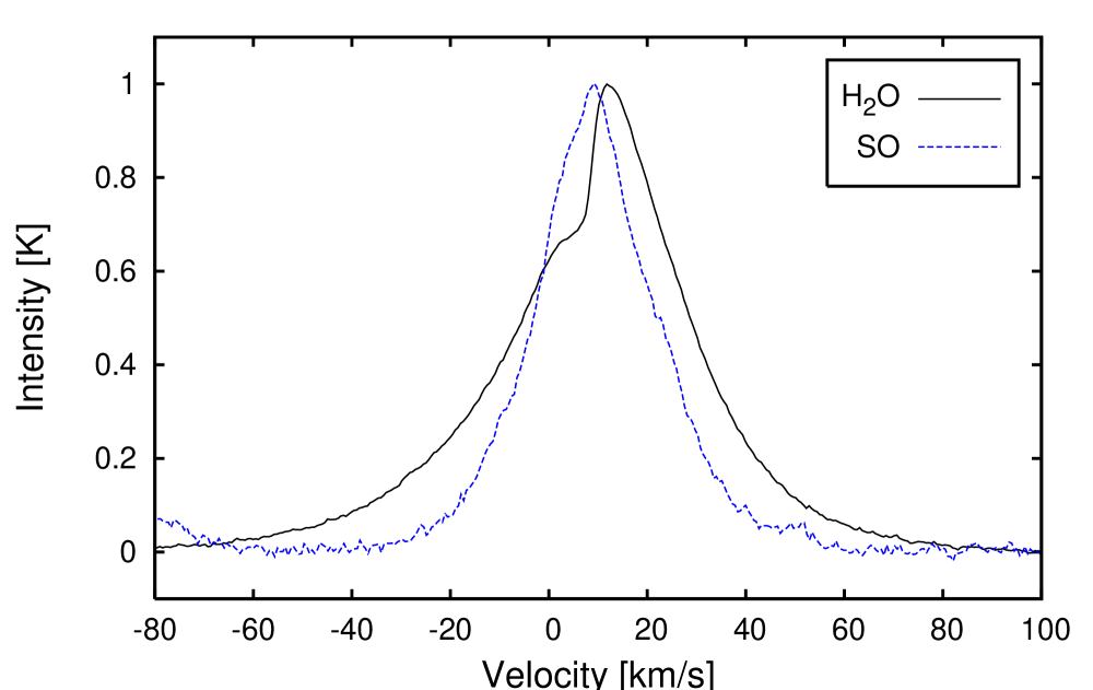
Figure 22: Comparison of the 13₁₃ – 12₁₂ SO transition and $o$-H₂O, both normalised with respective peak intensity. Both species show emission from the LVF and the HVF, but the water LVF is self-absorbed in the blue-shifted emission.

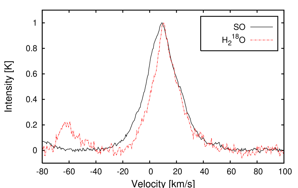
Figure 23: Comparison of the 13₁₃ – 12₁₂ SO transition, and $o$-H${}_{2}^{18}$O normalised with respective peak intensity.

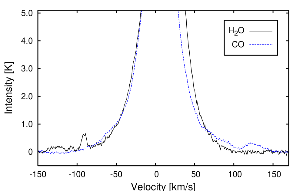
Figure 24: Comparison of the broad HVF emission in the line wings of CO and $o$-H₂O scaled 2.5 times. Note the large velocity scale.

However, our detected optically thin $p$-H₂O 6_2,4 – 7_1,7 transition with upper state energy 867 K, clearly reveals the emission from the HC. The width of the line is 12 km s^-1 at $\upsilon_{\mathrm{LSR}}\sim$4.4 km s^-1, between velocities $-$8 and 15 km s^-1. When column densities are calculated using the simple LTE approximation, we find values in the range (3.7 – 12)$\times 10^{18}$ cm^-2 for a temperature range of 200 – 500 K and a typical source size of 10$\arcsec$. Since no clear HC emission is seen from the ground rotational state transition in H${}_{2}^{17}$O, either the temperature in the HC is high enough to result in the negligible emission of this transition from the HC, or the H${}_{2}^{17}$O transition has an optically thick LVF emission which is blocking possible HC emission. If the temperature is 500 K, the emission from the HC would only be about 10% of the total (if no optical depths are taken into account), and therefore would be hidden in the stronger and broader LVF emission even if H${}_{2}^{17}$O is optically thin. However, if the temperature in the HC is about 200 K, the H${}_{2}^{17}$O LVF emission has to have an optical depth larger than unity. Since our estimated value is about 1.5, this is consistent with a HC temperature of 200 K and a column density of HC H₂O 1.2$\times 10^{19}$ cm^-2. This is in agreement with the only previous observation of H₂O emission from the HC made by S01. They detected the vibrationally excited 1_1,0 – 1_0,1 $v_{2}=1$ transition and found a HC column density of 3$\times 10^{19}$ cm^-2 with a temperature of 200 K and a water abundance of 1$\times 10^{-5}$. Gensheimer et al. (Gensheimer (1996)) estimated the HC H${}_{2}^{18}$O column density to be 2.7$\times 10^{16}$ cm^-2 from H${}_{2}^{18}$O mapping of the quasi-thermal 3_1,3 – 2_2,0 transition with the IRAM telescope (12$\arcsec$ beam). This column density translates to 1.3$\times 10^{19}$ cm^-2 for H₂O (corrected for source size and isotopologue ratio differences), in excellent agreement with our result, even though their observations suffered from severe blends. Their HC water mapping also showed that the emission from both H${}_{2}^{18}$O and HDO were unresolved by their beam, and the HDO mapping showed sizes of 6 – 8$\arcsec$.

Our tentative detection of the optically thin HC emitting $o$-H${}_{2}^{18}$O 4_2,3 – 3_3,0 transition, with an upper state energy of 430 K, results in a HC H₂O column density of about 4$\times 10^{19}$ cm^-2.

6.2.3 Comparisons of outflow column densities

Our column density results for the Plateau agrees excellently with those of Wright et al. (Wright 2000 (2000)), who observed 19 pure rotational lines in absorption using the Short Wavelength Spectrometer (SWS) on board the Infrared Space Observatory (ISO), with a beam size of 14$\arcsec\times 20\arcsec$ to 20$\arcsec\times 30\arcsec$. Their rotation diagram, including a generalised curve-of-growth method, results in a rotation temperature of 72 K, and a beam-averaged column density (from the total emission) of 1.5$\times 10^{18}$ cm^-2. They also conclude that the observed water arises from an outflow centred near IRc2.

Lerate et al. (Lerate (2006)) observed more than 70 far-IR pure rotational H${}_{2}^{16}$O lines, and 5 H${}_{2}^{18}$O lines, with the ISO LWS (Long Wavelength Spectrometer) between $\sim$43 and 197 $\mu$m (beam size about 80$\arcsec$). Their rotation diagram of the total emission from H${}_{2}^{18}$O results in a beam-averaged column density of (2 – 5)$\times 10^{14}$ cm^-2, and a rotation temperature of 60 K. For a 15$\arcsec$ outflow source, their result translates to (1.8 – 4.7)$\times 10^{18}$ cm^-2 for H${}_{2}^{16}$O, also in good agreement with our value. In the analysis by Cernicharo et al. (Cernicharo (2006)) of this data set, they concluded that most of the water emission and absorption arises from an extended flow of gas with velocity 25$\pm 5$ km s^-1, with an inferred kinetic gas temperature of 80 – 100 K.

6.2.4 HDO from the Compact Ridge, Low Velocity Flow and the Hot Core

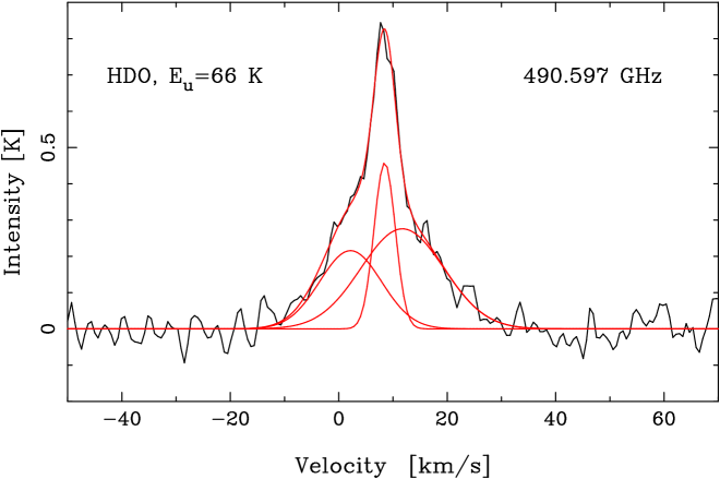
Figure 37: A three-component Gaussian fit to HDO shown together with the individual Gaussians. The line widths are 5 km s^-1, 13 km s^-1, and 18 km s^-1 for the CR, HC, and LVF, respectively.

The deuterated species HDO is observed in the 2_0,2 – 1_1,1 transition with $E_{u}$ = 66 K, and shows evidence of CR, LVF, and also HC emission as is observed by W03. Figure 37 shows a three-component Gaussian fit. Pardo et al. (Pardo (2001)) reported detections of the 2_1,2 – 1_1,1 and 1_1,1 – 1_0,0 lines in the 850 – 900 GHz spectral region, which seem to trace the Plateau gas and not the HC. Their conclusion is that the HC component is hidden behind the optically thick HDO LVF in their transitions, which is supporting our analysis of the non-detection of HC emission in the ground state rotational water transitions.

A T-line at 559.816 GHz tentatively is identified as the high energy (580 K) HDO transition 6_2,4 – 6_2,5.

Our estimated column density of HDO, assuming that the main emission originates in the outflows, is 9.1$\times$$10^{15}$ cm^-2, which is about the same value as reported by Lerate et al. (Lerate (2006)), $8.5\times 10^{15}$ cm^-2 (corrected for source size). The column density reported by Pardo et al. (Pardo (2001)) is higher, 5$\times 10^{16}$ cm^-2, calculated from an LVG model with a source size of 15$\arcsec$, and opacities of 3.7 and 6.7 for their two lines.

We also calculate the column densities for the CR, LVF and HC separately, which are found to be 1.8$\times 10^{16}$ cm^-2, 4.5$\times 10^{15}$ cm^-2, and 1.5$\times 10^{16}$ cm^-2, respectively. With correction for source-size, this is 2 – 4 times lower than found in Olofsson (HansOlofsson84 (1984)) by mapping the 1_1,0 – 1_1,1 transition with a 47$\arcsec$ beam (at Onsala Space Observatory); 3$\times 10^{16}$ cm^-2, 1$\times 10^{16}$ cm^-2, and 7$\times 10^{16}$ cm^-2, respectively.

6.2.5 Molecular abundance ratios

The [D/H] ratio calculated from from HDO/H₂O is 0.005, 0.001 and 0.03 in the LVF, HC, and CR, respectively (Table 6). The CR ratio may be compared to the HDCO/H${}_{2}^{13}$CO ratio from which we obtain a similar [D/H] value of 0.01 (see Sect. 4.6.1). Lerate et al. (Lerate (2006)) found [D/H] values in the range 0.004 – 0.01.

The column densities for H₂O and H₂S from the LVF are also used to estimate the molecular abundance ratio of O/S to $\sim$20 (Table 6). Using the H₂CS/H${}_{2}^{13}$CO ratio we obtain a similar value of $\sim$15 (see Sect. 4.5.2).

7 Molecular abundance estimates

7.1 Gas-phase abundances from the Odin spectral line survey

Our estimated abundances for each subregion are summarised in Table 3, together with comparison abundances mostly from B87 and S95. We find very high gas-phase abundances of H₂O, NH₃, SO₂, SO, NO, and CH₃OH. Note that both our LVF and HC abundances are source averages. S95 use beam-averaged abundances (with a HPBW of 14$\arcsec$), and B87 use a HC size of 10$\arcsec$ and a Plateau size of 20$\arcsec$, while we separate the LVF and HVF emissions with a slightly smaller size for the LVF (15$\arcsec$). The beam-averaged CR abundances in both B87 and S95 are corrected to our source-sizes to allow an easier comparison.

Table 3: Derived abundances and comparisons.

Region	Species	X${}^{\,g}$	B87 X${}^{\,h}$	S95 X${}^{\,i}$
		[$\times 10^{7}$]	[$\times 10^{7}$]	[$\times 10^{7}$]
LVF${}^{\,a}$	H2O	29
	HDO	0.15	0.17
	SO2	20	5.2	1.3
	SO	3.1	5.2	2
	SiO	0.11	0.28	0.08
	H2S	1.5	0.98
	H2CO	0.14	0.31	1.1
	CS	0.12	0.22	0.04
	HNC	0.012
HVF	H2O/Total H${}_{2}^{\,b}$	220	200-300${}^{\,j}$
	H2O/Hot H${}_{2}^{\,c}$	2900	2000-5000${}^{\,k}$
	SO2	225
	SO	21
	SiO	0.45
HC${}^{\,d}$	H2O	120	140${}^{\,l}$
	HDO	0.15	0.5	0.14
	H2S	0.27	0.3m
	CH3CN	0.05	0.078	0.04
	NH3	16	10${}^{\,n}$
	HC3N	0.018	0.016	0.018
	OCS	0.17		1.1
	CH3OH	7.9${}^{\,o}$	1-10${}^{\,p}$	1.4
	HNC	0.0044
	CS	0.029		0.06
	CN	0.079		0.008
	NO	2.8	2.0${}^{\,m}$
CR${}^{\,e}$	H2O	28
	HDO	0.87		0.93
	NH3	2.0
	CH3OH	120${}^{\,o}$	30	22
	(CH3)2O	6.5	2.5	1.0
	H2CO	1.0	0.6	0.46
	HDCO	0.014
	H2CS	0.065	0.06	0.014
	SO2	10
	SO	0.85
	CS as CR	0.40		0.1
ER${}^{\,f}$	CS as ER	0.21	0.025	0.11
	HNC	0.001	0.005
	N2H+	0.0005
PDR${}^{\,f}$	H2O	$\ga$1.1q	0.33r
	CN	0.02	0.03
	NH3	0.05s

• LVF $N$(H₂) = 3$\times 10^{23}$ cm^-2 (this work). ^bHVF total $N$(H₂) = 4$\times 10^{22}$ cm^-2 (this work). ^cHVF hot $N$(H₂) = 3$\times 10^{21}$ cm^-2 (Watson et al. Watson (1985)). ^dHC $N$(H₂) = 1$\times 10^{24}$ cm^-2 (B87). ^eCR $N$(H₂) = 2$\times 10^{23}$ cm^-2 (Wilson et al. Wilson86 (1986); Goldsmith et al. Goldsmith97 (1997)). ^fFor both the ER and PDR: $N$(H₂) = 2.0$\times 10^{22}$ cm^-2 (this work, see Sect. 5). ^gSource averages with sizes given in Tables 1 and 2. ^hSource averages from Blake et al. Blake (1987). ⁱSource averages from Sutton et al. Sutton (1995). ^jPlateau abundance (both LVF and HVF), Cernicharo et al. (Cernicharo (2006)). ^kWright et al. (Wright (1996)). ^lGensheimer et al. (Gensheimer (1996)). ^mC05. ⁿHermsen et al. (1988a ). ^oEstimated from the CH₃OH two-component rotation diagram. ^pMenten et al. (Menten (1988)). ^qW06. ^rMelnick et al. (Melnick (2000)). ^sLarsson et al. (Larsson (2003)) towards the Orion Bar.

A large source of uncertainty in these calculations is the adopted H₂ column densities. Whenever possible we have used our own calculated H₂ column densities (for the ER, LVF, HVF, Table 2). For the HC and CR we have adopted $N$(H₂) = 1$\times 10^{24}$ cm^-2 (calculated for a HC size of 10$\arcsec$ in B87), and $N$(H₂) = 2$\times 10^{23}$ cm^-2 (Wilson et al. Wilson86 (1986); B87; Goldsmith et al. Goldsmith97 (1997)), respectively. In case of the HVF we also compare the (shocked) water column with the column density of the hot (shocked) H₂, where $N_{\mathrm{HVF}}$ = 3$\times 10^{21}$ cm^-2 (Watson et al. Watson (1985)). When we calculate the abundances we assume that the derived H₂ column density spatially coincides with the emission from the species of interest.

Most of our abundances, listed in Table 3, are in very good agreement with B87 and S95. However, there are a few exceptions – a 4 – 15 times higher abundance for SO₂ in the LVF, and 2 – 5 times higher abundances in general in the CR than in B87 and S95. The differences may arise because our observed transitions probe higher density and more compact regions in the CR. Since we cannot discriminate between CR or ER emission for CS, the abundance is calculated with both alternatives. It turns out that the CS abundance is about the same for either source of emission. However, the high ER abundance of CS compared to that of B87 is to a large extent due to the very different H₂ column densities used in our survey and B87, $N$(H₂) = 2$\times 10^{22}$ cm^-2 and $N$(H₂) = 3$\times 10^{23}$ cm^-2, respectively.

Our HVF H₂O abundance, as compared to the total H₂ density in the flow, is 3$\times 10^{-5}$, in agreement with the water abundance in the Plateau estimated by Cernicharo et al. (Cernicharo (2006)). If we compare the HVF water abundance to the hot shocked H₂ it is consistent with Wright et al. (Wright 2000 (2000)) and Melnick et al. (Melnick (2000)), who estimate the shocked Plateau water abundance to be (2 – 5)$\times 10^{-4}$.

The HC H₂O abundance is in agreement with the mapping of H${}_{2}^{18}$O towards the Orion Hot Core with the IRAM telescope (12$\arcsec$ beam) by Gensheimer et al. (Gensheimer (1996)). Their estimated abundance is 1.4$\times 10^{-5}$. S01 estimate the water abundance to be $\sim$1.0$\times 10^{-5}$ from their observation of the vibrationally excited H₂O 1_1,0 – 1_0,1 $v_{2}$=1 transition, also in accordance with our value.

High water abundances in high temperature regions, for example in outflows, PDRs, and hot cores are consistent with both water and deuterated water forming on grains at low temperatures, and subsequently evaporating from the grain surfaces at high temperatures above $\sim$90 K. At temperatures above $\sim$400 K, easily reached in shocks, neutral-neutral reactions produce even higher water abundances (cf. Neufeld et al. Neufeld95 (1995)). Hence, our high abundance in the HC of H₂O can be the result of evaporation from grain surfaces, which also applies to CH₃OH and NH₃, as is discussed in more detail in Sect. 7.2. The water abundance in the CR and LVF is about the same, and lower than in the HC. This might be a natural consequence of a lower temperature in these regions with less evaporation from grain surfaces, which also applies to the PDR region. This is also the cause of the non-detection of water in the ER which has a temperature below the sublimation temperature. The highest water abundance is found in the HVF, which is suggestive of an even more efficient production in shocks.

Table 4: Relative abundances ratios and comparisons with ice abundances.

Abundance ratio	LVF	HC	CR	Ice abundancesa
	$N$/$N$(H2O)$\times$100			Orion IRc2	W33A
CH3OH/H2O		7	430	10	11 – 17
HDO/H2O	0.52	0.13	3.2		0.3
HDCO/H2CO			1.2
NH3/H2O		13	7		15
SO2/H2O	69		36		$\sim$1.6
H2CO/H2O	0.5		3.6		$\sim$3
SO/H2O	11		3.0
OCS/H2O		0.14		$<$0.2	0.2
CS/H2O	0.41	0.02	1.4
H2S/H2O	5.2	0.22

• ^aGibb et al. (Gibb00 (2000)) and (Gibb04 (2004)).

7.2 Gas-phase vs grain surface abundances

Ratios of our observed gas-phase column densities in the Orion LVF, HC and CR sources (as derived from Tables 1 and 2) and the water column density is found in Table 4. These ratios are compared with the corresponding grain-surface abundance ratios towards two of the sources observed by ISO (Gibb et al. Gibb00 (2000), Gibb04 (2004)), Orion IRc2 and the embedded high-mass protostar W33A.

Some suggestions from these comparisons are:

• Both CH₃OH and H₂O are very abundant in the dense and warm HC, and their gas-phase abundance ratio is very similar to that in the grain-surface ice of Orion IRc2 and W33A. This strongly points at a dominant production via hydrogenation on cold grain surfaces and subsequent evaporation in the warm and hot cores (cf. Brown et al. Brown88 (1988); Caselli et al. Caselli93 (1993); Stantcheva and Herbst Stantcheva and Herbst 04 (2004); Garrod & Herbst Garrod and Herbst06 (2006); Chang et al. Chang Cuppen and Herbst 07 (2007)), especially so since gas-phase production of CH₃OH has been shown to be very inefficient (cf. Geppert et al. Geppert (2005); Millar Millar (2005); Garrod et al. Garrod Wakelam and Herbst 07 (2007)). In the CR the CH₃OH/H₂O ratio is about 60 times higher than in the HC and in ices, caused by the four times decrease of the water abundance, and the 15 times higher methanol abundance as compared to the HC. This may suggest that H₂O is consumed in the formation of CH₃OH in accordance with the recent laboratory study of methanol formation from electron-irradiated mixed H₂O/CH₄ ice at 10 K by Wada et al. (Wada Mochizuki and Hiraoka 06 (2006)).

• The rather similar gas-phase HDO/H₂O abundance ratios in the LVF and HC compared with the ice ratio in W33A most likely suggest efficient deuteration reactions on grain surfaces as the cause of the high water deuteration level. This is supported by our previous conclusions about the grain surface origin of the high water abundances. The much higher HDO/H₂O ratio found in the CR, as well as the similar HDCO/H₂CO ratio, at least partly is caused by a decreasing H₂O abundance – possibly a result of H₂O consumption in the efficient grain-surface formation of CH₃OH in this source.

• Likewise, the gas-phase abundance ratios of NH₃ and H₂O in the CR and HC are similar to the W33A ice abundance ratio, again strongly suggesting that both these abundant species originate primarily from hydrogenation on cold grain surfaces with subsequent evaporation (cf. Stantcheva and Herbst Stantcheva and Herbst 04 (2004); Garrod et al. Garrod Wakelam and Herbst 07 (2007)).

• The high SO₂/H₂O abundance ratio observed in the LVF is contrasted with a low ice ratio in W33A. The latter ratio is most likely explained by rather inefficient gas-phase formation of SO₂ and subsequent adsorption onto already icy grain mantles formed by efficient hydrogenation on the cold grains. The high gas-phase H₂O abundance in the LVF may directly result from evaporation caused by the strong radiation from the nearby LVF driving source. This heating also could release S and Si atoms from the grains. Subsequent gas-phase reactions, based upon undepleted elemental abundances, then could lead to the elevated abundances of SO₂, SO, H₂S and SiO observed in the LVF. These abundances are several orders of magnitude higher than those in quiescent clouds where the abundances of S and Si appear to be depleted (B87; Irvine et al. Irvine87 (1987)). In this scenario the ISO observations of OH at high abundance in the LVF (Goicoechea et al. Goicoechea (2006)) are important. Low velocity shocks also may play a role here (cf. Mitchell Mitchell84 (1984); Pineau des Forêts et al. Pineau des Foretes93 (1993)).

• The very similar CR H₂CO/H₂O gas-phase and W33A ice abundances most likely just tells us that both abundance ratios have the same main origin.

• The similarity of the HC gas-phase OCS/H₂O abundance ratio and the corresponding ratio in the W33A ice, also might hint at a grain surface origin of OCS. However, the comparatively low OCS abundance is accommodated by current ion-molecule reaction models and the ice content then likely is a result of adsorption.

8 Discussion – source sizes & source structure

We have in our column density and molecular abundance calculations in all cases treated the various Orion KL subregions, probed by the large Odin antenna beam, as homogeneous sources having specified average temperatures, densities and equivalent circular sizes and beam-filling factors.

However, the High Velocity Outflow is known to be bi-polar with a FWHP size of 60 – 70″, as estimated from simultaneous Odin mapping of the H₂O and CO $J$ = 5 – 4 brightness distributions (Olofsson et al. 2003a , Hjalmarson et al. Hjalmarson05 (2005)). As seen from the radiative transfer equation, the H₂O excitation temperature corresponding to a size of 70″ is only 26 K, while a temperature of 72 K as found by Wright et al. (Wright 2000 (2000)) corresponds to a size of only 32″. This indicates a very clumpy H₂O brightness distribution, and that this source is filled with approximately one fourth of water emission. Similar results are obtained investigating the size-temperature relation of CO. In fact, the appearance of the HVF may be similar to the clumpy, finger-like emission seen in shock-excited H₂ (Salas et al. Salas (1999)).

The Low Velocity Outflow has a NE-SW elongated structure, roughly orthogonal to the HVF, which also must have small scale structure (Genzel et al. Genzel81 (1981); Greenhill et al. Greenhill98 (1998)). If we guide ourselves by the optically thick HDO lines observed by Pardo et al. (Pardo (2001)) and use a HPBW size of 15″ for H${}_{2}^{18}$O, the corresponding excitation temperature is only 40 K. The size corresponding to 72 K is 10$\arcsec$ which suggests that this source is filled with about one half of radiating gas-phase water. Similar results are found for all optically thick outflow species.

The Compact Ridge and Hot Core size-temperature relations are more consistent with the assumed values, although we know from Beuther et al. (Beuther (2005)) that both sources are very clumpy. This might be caused by their much smaller size as compared to the outflows, where the clumping affects larger scales. As seen from the CH₃OH Fig. 46 (on-line material) and Fig. 12, the source size of the CR also varies with the upper state energies of the lines. This might indicate considerable temperature and density variations within the CR.

Considering the uncertainties discussed above and in Sect. 3 and 10.2 (Appendix), the striking agreement with B87 and S95 strengthens our confidence of our results.

9 Summary

We present first results from a spectral line survey towards Orion KL in a frequency range inaccessible from the ground covering 487 – 492 and 542 – 577 GHz.

Some of the results from this survey:

1. We detect a total of 280 lines from 38 different molecular species.

2. In addition we detect 64 unidentified lines, which represents 19$\%$ of the total. Some tentative assignments of a few of them have been made such as the interstellar anion SH^-, ND, SO⁺, and CH₃OCHO.

3. The total beam-averaged emission in our survey is dominated by CO, $o$-H₂O, SO₂, SO, ¹³CO and CH₃OH. Species with the largest number of lines are CH₃OH, (CH₃)₂O, SO₂, ¹³CH₃OH, CH₃CN and NO.

4. Six water lines are detected, including the ground state rotational transition 1_1,0 – 1_0,1 of $o$-H₂O, and its isotopologues $o$-H${}_{2}^{18}$O and $o$-H${}_{2}^{17}$O, which shows emission from the Low- and High Velocity Flow and the Compact Ridge. Hot Core emission from water is observed from the $p$-H₂O transition 6_2,4 – 7_1,7 with an upper state energy 867 K, and from a weak line feature at 489.054 GHz identified as the 4_2,3 – 3_3,0 transition of $o$-H${}_{2}^{18}$O with an upper state energy of 430 K. We have also observed the HDO 2_0,2 – 1_1,1 transition from the Low Velocity Flow, Compact Ridge and the Hot Core, and have a tentative detection of the high energy transition (581 K) 6_2,4 – 6_2,5 of HDO.

5. We detect the 1₀ – 0₀ transitions of NH₃ and the isotopologue ¹⁵NH₃. The main isotopologue shows emission from both the Hot Core, LVF and Compact Ridge, while the rarer isotopologue only exhibits emission from the Hot Core.

6. Isotopologue abundance ratios of D/H, ¹²C/¹³C, ³²S/³⁴S, ³⁴S/³³S and ¹⁸O/¹⁷O are calculated, as well as the molecular abundance ratio of O/S, all in agreement with previous findings.

7. Different methods are used to obtain rotation temperatures and column densities. For eight different species with at least four lines and a sufficient energy range in the transitions, the rotation diagram method and the forward model are applied. The LTE approximation is used for all the other species.

8. Abundances are estimated for the observed species from the different subregions, and we find very high gas-phase abundances of H₂O, NH₃, SO₂, SO, NO, and CH₃OH. An important fact here is that all our abundance determinations, including those for water vapour, are based upon the same methodology.

9. A comparison of our estimated gas-phase abundances with the ice inventory of ISO is shedding new light on the chemical origins of H₂O, CH₃OH, NH₃ and SO₂ in the various Orion KL subregions.

10. The line density in our survey is 4 – 20 per GHz, with a mean of 8 per GHz. This is comparable with larger telescopes ($\sim$10 GHz^-1), showing the excellent performance of the Odin satellite.

10 Data analysis methods

10.1 Single line analysis

With the assumption of optically thin emission, neglecting the background radiation, and assuming that the source fills the antenna main beam, the beam averaged upper state column density is calculated as

$$N_{{u}}^{\mathrm{\,thin}}=\frac{8\pi k\nu_{{ul}}^{2}}{hc^{3}}\frac{1}{A_{{ul}}}\int{T_{\mathrm{mb}}}\,\mathrm{d}\upsilon,$$ (8)

where $k$ is the Boltzmann constant, $\nu_{{ul}}$ is the frequency of the transition, $h$ is the Planck constant, $c$ is the speed of light, $A_{{ul}}$ is the Einstein $A$-coefficient for the transition, and $T_{\mathrm{mb}}$ is the main beam brightness temperature. As customary the frequency axis $\nu$ has been converted to a velocity axis $\upsilon$ using the speed of light.

The total column density of each species can then be found assuming LTE (Local Thermodynamic Equilibrium), where the excitation temperatures, $T_{\mathrm{ex}}$, for all the energy levels are the same. The molecular population of each level is then given by the Boltzmann equation, which also defines $T_{\mathrm{ex}}$

$$N_{u}=N_{\mathrm{tot}}\frac{g_{u}}{Q(T)}\,e^{-E_{u}/kT_{\mathrm{ex}}},$$ (9)

where $g_{u}$ is the statistical weight of the upper state, and $Q(T)$ is the partition function, which only depends on temperature and molecular constants and hence differs for different kinds of species. The $A$-coefficients, statistical weights, partition functions and upper state energy levels are available via the databases JPL, CDMS, Leiden (Schöier et al. Schoier (2005)) or SLAIM$\emptyset$3. For a few molecules, e.g. (CH${}_{3})_{2}$O, we calculate the $A$-coefficients using line strengths found in SLAIM$\emptyset$3 as

$$A_{ul}=\frac{16\,\pi^{3}\,\nu_{ul}^{3}\,\mu^{2}}{3\,\epsilon_{0}\,h\,c^{3}}\frac{S_{ul}}{g_{u}}$$ (10)

where $S_{ul}$ is the rotational part of the line strength, and $\mu$ is the molecular dipole moment.

From Eq. (9) and (1), we obtain the beam-averaged total column density

$$N_{\,\mathrm{tot}}^{\,\mathrm{thin}}=\frac{8\pi k\nu_{{ul}}^{2}}{hc^{3}}\frac{1}{A_{{ul}}}\frac{Q(T)}{g_{{u}}}e^{\,E_{{u}}/kT_{\mathrm{ex}}}\int{T_{\mathrm{mb}}}\,\mathrm{d}\upsilon$$ (11)

assuming optically thin emission.

The solution of the radiative transport equation, neglecting background radiation and with a constant source function, is

$$T^{*}_{\mathrm{A}}=T_{\mathrm{b}}\,\eta_{\mathrm{mb}}\,\eta_{\mathrm{bf}}=J(T_{\mathrm{ex}})\,(1-e^{-\tau})\,\eta_{\mathrm{mb}}\,\eta_{\mathrm{bf}},$$ (12)

where the beam-filling factor $\eta_{\mathrm{bf}}=\theta_{\mathrm{s}}^{2}/(\theta_{\mathrm{s}}^{2}+\theta_{\mathrm{mb}}^{2})$, assuming that both the source brightness distribution and the antenna response are circularly symmetric and Gaussian. The radiation temperature, $J(T_{\mathrm{ex}}$) is

$$J(T_{\mathrm{ex}})=\frac{h\nu}{k}\frac{1}{e^{\,h\nu/kT_{\mathrm{ex}}}-1}\approx T_{\mathrm{ex}},$$ (13)

where the approximation is valid only if h$\nu$ $\ll$ k$T_{\mathrm{ex}}$. For the appropriate temperatures in this region, $T\approx$ 100 – 200 K, and frequencies $\sim$550 GHz, the radiation temperature will differ from $T_{\mathrm{ex}}$ by approximately 10 – 15%. Accordingly, we use $J(T_{\mathrm{ex}}$) and not $T_{\mathrm{ex}}$ in our calculations.

If the emission is optically thick ($\tau\gg$1) Eq. (12) simplifies to

$$T^{*}_{\mathrm{A}}=J(T_{\mathrm{ex}})\,\eta_{\mathrm{mb}}\,\eta_{\mathrm{bf}}=J(T_{\mathrm{ex}})\,\eta_{\mathrm{mb}}\,\frac{\theta_{\mathrm{s}}^{2}}{\theta_{\mathrm{s}}^{2}+\theta_{\mathrm{mb}}^{2}}.$$ (14)

Using this equation the beam-filling, and hence the approximate source size, can be determined without relying on correctly calculated optical depths. The variation in $T^{*}_{\mathrm{A}}$ that is seen mainly will be due to variations in the beam-filling factor, but there can also be variations in $T_{\mathrm{ex}}$, both along the path and between different states, which cannot be determined.

Since molecular clouds are known to be clumpy down to very small scales, it is indeed likely that the source does not fill the beam. This is especially true in case of the large Odin beam, and the total column density from Eq. (11) will be too low by a factor of 1/$\eta_{\mathrm{{bf}}}$. Variations in beam-filling between the different transitions of the same molecule also are probable. Hence, when we are comparing other observations (e.g. interferometry mapping) with ours to estimate the beam-filling, by necessity we have to compare transitions with similar parameters tracing the same gas.

The optical depth at the centre of the line can be calculated, assuming LTE and a Gaussian line profile, using

$$\tau_{\mathrm{max}}=\sqrt{\frac{\ln\,2}{16\,\pi^{3}}}\frac{c^{3}}{\nu_{{ul}}^{3}\,\Delta\upsilon}\,A_{{ul}}\,N_{\mathrm{tot}}\,\frac{g_{u}}{Q(T)}\,e^{-E_{u}/kT_{\mathrm{ex}}}\,(e^{\,h\nu_{{ul}}/kT_{\mathrm{ex}}}-1)\\$$ (15)

where $\Delta\upsilon$ is the width of the line, and $E_{u}$ is the upper state energy. However, this approach demands knowledge of the total column density. If we have observations of isotopologues, and if the isotopologue abundance ratio $R$ is known, then the optical depths can be determined by means of Eq. (12). If the excitation temperatures are about the same for both isotopologues, and the optical depth of isotopologue one is larger than isotopologue two by a factor $R$, we then will have

$$\frac{T_{\mathrm{A,1}}}{T_{\mathrm{A,2}}}=\frac{(1-e^{-\tau_{1}})\,\eta_{\mathrm{\,bf,1}}}{(1-e^{-\tau_{2}})\,\eta_{\mathrm{\,bf,2}}}=\frac{(1-e^{-R\,\tau_{2}})\,\eta_{\mathrm{\,bf,1}}}{(1-e^{-\tau_{2}})\,\eta_{\mathrm{\,bf,2}}}.$$ (16)

This will give the mean optical depths of both species. If the emissions are co-spatial the beam-filling factors cancel.

Once a transition has become optically thick, the value of $N_{u}$/$g_{u}$ cannot increase any further. The derived total column density will then be too low and needs an optical depth correction factor $C_{\tau}$, which will be one or larger

$$C_{\tau}=\frac{\tau}{1-e^{-\tau}}.$$ (17)

With corrections for optical depth and beam-filling the true total source averaged column density will be

$$N_{\mathrm{tot}}=\frac{C_{\tau}}{\eta_{\mathrm{bf}}}\,\frac{8\pi k\nu_{{ul}}^{2}}{hc^{3}}\frac{1}{A_{{ul}}}\frac{Q(T)}{g_{{u}}}e^{E_{{u}}/kT_{\mathrm{ex}}}\int{T_{\mathrm{mb}}}\,d\upsilon=\frac{C_{\tau}}{\eta_{\mathrm{bf}}}\,N_{\,\mathrm{tot}}^{\,\mathrm{thin}}.$$ (18)

If no information about optical depth is available this correction is not taken into account. For the excitation temperature in Eq. (14) and (18), we use an adopted temperature that fits the species (Table 1), or the calculated rotation temperature $T_{\mathrm{ROT}}$ (see Sect. 3.2.1).

Note the importance of the partition function $Q(T)$, and the statistical weight $g_{u}$ in Eq. (18). If the statistical weights include the $ortho$/$para$ ratio whenever these molecular sub-divisions exist, the partition function must include them. It is also important to use the same statistical weights $g_{u}$ in Eq. (18) when the partition function $Q(T)$ is calculated.

10.2 Additional limitations

If there are deviations from the basic assumptions, errors will occur in the calculations for all models (cf. Goldsmith and Langer Goldsmith Langer (1999)). These effects can to some extent be corrected for, like optical depth effects and beam-filling, as discussed above. In addition we have:

1. Several excitation temperatures/Non-LTE. The population distribution may not be characterised by a single rotational temperature. The temperature can vary due to density, excitation gradients along the line-of-sight, IR flux, subthermal excitation etc. Since our beam is very large and encompasses a variety of different conditions, we may expect emission from several different sources, each with different temperature.

2. Adopted excitation temperature. Whenever we have too few lines to use the rotation diagram method or forward model we use the LTE approximation for a single line. The excitation temperature is then adopted from a rotation temperature of a similar species in our survey, or taken from the literature. This can create errors if the adopted temperature is not appropriate.

3. Source structure. The beam-filling correction are calculated assuming a homogenous source (see also Sect. 8). Clumping and substructures can introduce errors in the beam-filling corrections. Vastly different opacitites between the isotopologues (with NH₃ and H₂O as good examples) also complicate the analysis, as the beam-filling factors may be very different.

4. Gaussian decomposition. Errors in our Gaussian decompositions can introduce errors in the calculated optical depths and the column densities.

5. H₂ column densities. The largest source of uncertainty in the abundances in Sect. 7 is the adopted H₂ column densities and the assumption that the H₂ emission and the molecule of interest spatially coincides. This can create errors by orders of magnitude.

6. Observational errors. Errors may exist in the measured line intensities due to misidentifications, unresolved blends, or pointing and calibration. However, the errors must be rather large to create significant errors in the column density obtained from the rotation diagram and forward model.

7. Background radiation. The background radiation, e.g. emission from warm dust, may be too large to be neglected. If the condition $T_{\mathrm{ex}}\gg T_{\mathrm{bg}}$ is violated, shifts along the ordinate in the rotation diagram with a factor of $\ln$ (1$-T_{\mathrm{bg}}$/$T_{\mathrm{ex}}$) will occur. The dust continuum radiation will for example affect the level populations of water, and must be included in accurate calculations for these transitions.

10.3 Determination of relative chemical abundances

The definition of molecular abundance of a species with respect to H₂ is the ratio of the volume densities. This demands detailed knowledge of the geometry of the emitting region. If this is not known, column densities can be used as a substitute, with the assumption that the two species are well mixed and emitted from the same region, to obtain average abundances along the line of sight

$$X_{\mathrm{species}}=\frac{N_{\mathrm{species}}}{N_{\mathrm{H_{2}}}}.$$ (19)

The use of column densities will provide a higher degree of accuracy than the use of volume densities (Irvine et al. Irvine85 (1985)). As long as the molecules are emitted from the same region with approximately the same source size, there is no dependence of beam-filling. In addition, since we have a uniformly calibrated set of data, uncertainties in calibration will not affect the result.

The relative isotopologue abundance $R$ can be determined in the same way as the molecular abundances,

$$R=\frac{N_{1}}{N_{2}},$$ (20)

when we have observations of optically thin isotopologues, or opacity-corrected column densities.

10.4 Optical depth broadening

If the intrinsic line shape is Gaussian, a high line opacity will increase the observed line width (cf. Phillips et al. Phillips79 (1979)) as

$$\Delta\upsilon\approx\Delta\upsilon_{i}\,\left(\frac{\ln\tau_{p}}{\ln 2}\right)^{1/2}$$ (21)

where $\Delta\upsilon_{i}$ is the intrinsic velocity width of the line and $\tau_{p}$ ($\gg$1) is the peak optical depth in the line.

Figure 25: Top figure shows the NH₃ line, the second figure shows four times magnified NH₃ line wings. The NH₃ line profile shows emission from the CR and HC. The ¹⁵NH₃, CH₃CN, HC₃N and OCS transitions suggest emission from the HC, and H₂S from both the HC and LVF. An intensity scale factor is given after the molecular species.

Figure 26: CO, isotopologues and atomic C. Note the different intensity scales.

Figure 27: SO and isotopologues. The SO line in the top panel is optically thick, and shows clear HVF line wings. The low-energy SO transition is optically thin. An intensity scale factor is given after the molecular species.

Figure 28: The $J$ = 13 – 12 transition for both SiO and ²⁹SiO. The SiO line is optically thick and also exhibits pronounced HVF line wings. A blend from CH₃OH and ¹³CH₃OH is visible at 19.6 km s^-1 in the SiO line. An intensity scale factor is given after the molecular species.

Figure 29: SO₂ with different upper state energy levels and A-coefficients. The ³⁴SO₂ line is the same transition as the SO₂ transition with $E_{u}$=80 K. An intensity scale factor is given in the top left corners.

Figure 30: ¹³CH₃OH with emission from the CR. An intensity scale factor is given in the top left corners, upper state energies given in K and $A$-coefficients in s^-1.

Figure 31: The line profile of HNC shows emission from the ER, HC and LVF, CN from the PDR/ER and HC, and N₂H⁺ from the ER. The line at v$\approx-$8 km s^-1 next to N₂H⁺ is OCS, which is also shown in Fig. 25. An intensity scale factor is given after the molecular species.

Figure 32: CH₃OH with emission from both the CR and HC. Vibrationally excited transitions are marked by $*$ after the intensity scale factor given in the top left corners, with upper state energies given in K and $A$-coefficients in s^-1.

Figure 33: The optically thick line profile of H₂CO show emission from the CR and LVF. The optically thin transitions of H${}_{2}^{13}$CO, HDCO, and H₂CS show only emission from the CR. The CS line profile shows emission from the HC, LVF and a narrow component from the CR or ER. An intensity scale factor is given after the molecular species, the upper state energies are given in K and the $A$-coefficients in s^-1.

Figure 34: Identification suggestions for a few U-lines together with ¹⁵NH₃, H₂S and CH₃CN as comparison lines. The U-line at 542.945 GHz is our strongest non-identified U-line. An intensity scale factor is given after the molecular species.

Figure 39: Ratio of $o$-H₂O over $o$-H${}_{2}^{18}$O.

Figure 40: Ratio of $o$-H${}_{2}^{18}$O over $o$-H${}_{2}^{17}$O.

¹³CH₃OH producing $T_{\mathrm{ROT}}$ = 115 K and $N_{\mathrm{ROT}}$ = 5.9$\times 10^{17}$ cm^-2 (extended source).

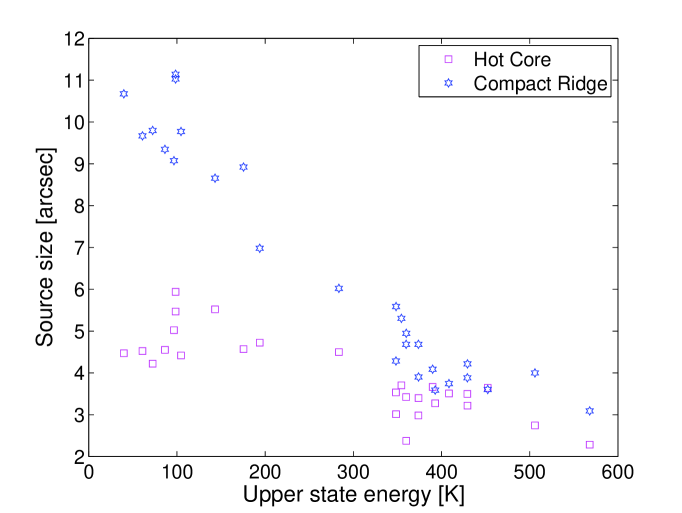
Figure 47: Source size variation with energy for two components of CH₃OH with no opacity correction.

Table 5: Summary of all detected species.

Species	Number	Upper state	$\int{T^{\,*}_{\mathrm{A}}\mathrm{d}\upsilon}$
	of lines	energy range
		[K]	[K km s-1]
CH3OCH3	47	106 – 448	18.3
SO2	42	75 – 737	239.9
34SO2	5	79 – 457	2.6
SO	5	71 – 201	181.5
33SO	3	191 – 199	6.5
34SO	2	191 – 197	15.6
CH3OH $v_{\rm t}$=1	42	332 – 836
CH3OH	34	38 – 863	108.6
13CH3OH	21	37 – 499	6.8
13CH3OH $v_{\rm t}$=1	2	373 – 670
CH3CN	17	410 – 1012	9.3
NO	12	84 – 232	11.1
CN	8	54	8.5
H2CS	5	138 – 343	1.7
H2CO	3	106 – 133	38.5
H${}_{2}^{13}$CO	1	130	0.6
HDCO	3	114 – 141	2.8
OCS	3	604 – 658	1.3
$o$-H2O	1	61	320.3
$p$-H2O	1	867	2.2
$o$-H${}_{2}^{17}$O	1	61	9.4
$o$-H${}_{2}^{18}$O	2	60 – 430	16.2
HDO	1	66	10.7
HC3N	2	648 – 799	0.6
CO	1	83	1 100
13CO	1	79	174.3
C17O	1	81	6.0
C18O	1	79	24.3
C	1	24	38.7
NH3	1	27	20.6
15NH3	1	27	0.7
HNC	1	91	10.7
N2H+	1	94	1.5
H2S	1	166	4.4
CS	1	129	24
13CS	1	173	v blend
SiO	1	190	17.6
29SiO	1	187	1.4
30SiO	1	185	0.5
HCS+	1	186	v blend
NS	1	442	v blend
U-line	28		9.1
T-line	36		7.2
No. of species	38
No. of lines	344
Total $\int{T^{\,*}_{\mathrm{A}}}\mathrm{d}\upsilon$			2 455

Table 6: Isotopologue abundance ratios from our survey, or from the literature, as compared to terrestrial values. The molecular abundance O/S ratios are also included.

	[12C/13C]	[32S/34S]	[34S/33S]	[18O/17O]	[16O/18O]	[D/H]	[O/S]	[14N/15N]	[28Si/29Si]
This survey	57$\pm$14${}^{{\,a}}$	21$\pm$6${}^{{\,b}}$ – 23$\pm$7${}^{\,c}$	4.9${}^{{\,d}}$	3.6${}^{{\,e}}$		0.001f– 0.03${}^{{\,g}}$	15${}^{{\,h}}$– 20${}^{{\,i}}$
Terrestrial	89j	22.5j	5.5j	5.5k			35v	273l	19.6${}^{{\,m}}$
K88j	47${}^{+6}_{-5}$	20.2${}^{+2.6}_{-2.1}$	5.7${}^{+0.8}_{-0.6}$
W&R94n	77$\pm$7	$\sim$22		3.2$\pm$0.2	560$\pm$25			450$\pm$22
C96o	75$\pm$21	35$\pm$10	7.53$\pm$0.45
B01p	65.0$\pm$9.2			4.15$\pm$0.59
P81bq				3.9$\pm$0.2
Various surveys	43$\pm$7r			4.17$\pm$0.26${}^{\,s}$	330$\pm 69^{\,{t}}$	2$\times 10^{-5}$ u			16.9$\pm 2.0^{{\,m}}$

• ^aFrom ¹²CH₃OH/¹³CH₃OH. ^bFrom ³²SO/³⁴SO. ^cFrom ³²SO₂/³⁴SO₂. ^dFrom ³⁴SO/³³SO. ^eFrom C¹⁸O/C¹⁷O. ^fFrom HDO/H${}_{2}^{17}$O Hot Core. ^gFrom HDO/H${}_{2}^{17}$O Compact Ridge. ^hFrom H${}_{2}^{13}$CO/H${}_{2}^{12}$CS CR. ⁱFrom H${}_{2}^{17}$O/H₂S LVF. ^jKahane et al. (Kahane (1988)), the envelope of IRC+10216. ^kBlake et al. (Blake (1987)). ^lHo & Townes (Ho and Townes (1983)). ^mPenzias (1981a ). ⁿWilson & Rood (Wilson and Rood (1994)) and references therein, local ISM. ^oChin et al. (Chin (1996)), towards Orion KL. ^pBensch et al. (Bensch (2001)), towards $\rho$ Ophiuchi Molecular Cloud. ^qPenzias (1981b ), towards Orion A. ^rSavage et al. (Savage (2002)), towards Orion A using CN and ¹³CN. ^sWouterloot et al. (Wouterloot (2005)), towards $\rho$ Ophiuchi Molecular Cloud, value from LTE column densities. ^tOlofsson (2003b ), from S¹⁸O observations of molecular cloud cores. ^uNeufeld et al. (Neufeld06 (2006)). ^v Standard abundances, Grevesse et al. (Grevesse (1996)).

Table 7: H₂O and isotopologue parameters and derived column densities.

Species	Compa	$\upsilon_{\mathrm{LSR}}$	$\Delta\upsilon$	$T^{\,*}_{\mathrm{A}}$	$T_{\mathrm{k}}$	Size	$N^{b}$	$\tau$	$N^{c}_{\tau\,\mathrm{corr}}$	$N_{\mathrm{ISO}}^{d}$
		[km s-1]	[km s-1]	[K]	[K]	[$\arcsec]$		cm-2]	cm-2]	[cm-2]
$o$-H${}_{2}^{16}$O	Total				72	(15)e		$\sim$1100f		1.7$\times 10^{18}$
	CR				115	(6)e		$\sim$860f		5.6$\times 10^{17}$
	LVF				72	(15)e		$\sim$1900f		8.7$\times 10^{17}$
	HVF	5.3	67.1	2.452	72	70	8.7$\times 10^{14}$	$\sim$910f	8.0$\times 10^{17}$	8.8$\times 10^{17}$
$p$-H${}_{2}^{16}$O	HC	4.4	12.0	0.181	200	10	1.2$\times 10^{19}$	0.3g
$o$-H${}_{2}^{17}$O	Total				72	15	8.6$\times 10^{14}$	0.9f	1.3$\times 10^{15}$
	CR	9.9	5.0	0.076	115	6	3.2$\times 10^{14}$	0.7f	4.4$\times 10^{14}$
	LVF	8.7	18.0	0.214	72	15	3.5$\times 10^{14}$	1.5f	6.7$\times 10^{14}$
	HVF	13.4	30.1	0.179	72	15	4.9$\times 10^{14}$	0.7f	6.8$\times 10^{14}$
$o$-H${}_{2}^{18}$O	Total				72	15	1.4$\times 10^{15}$	3.4f	5.0$\times 10^{15}$	5.0$\times 10^{15}$
	CR	10.1	5.0	0.145	115	6	6.2$\times 10^{14}$	2.6f	1.8$\times 10^{15}$	1.7$\times 10^{15}$
	LVF	10.5	18.0	0.275	72	15	4.6$\times 10^{14}$	5.9f	2.7$\times 10^{15}$	2.6$\times 10^{15}$
	HVF	13.4	33.4	0.298	72	15	9.3$\times 10^{14}$	2.8f	2.8$\times 10^{15}$	2.7$\times 10^{15}$
HDO	Total				72	15	9.1$\times 10^{15}$	$\sim$1.5g
	CR	8.5	4.6	0.459	115	6	1.8$\times 10^{16}$	$\sim$3g
	LVF	11.8	18.0	0.273	72	15	4.5$\times 10^{15}$	$\sim$0.3g
	HC	2.2	13.4	0.216	200	10	1.5$\times 10^{16}$	$\sim$0.5g

• Total=the total integrated intensity is used, CR=Compact Ridge, LVF=Low Velocity Flow, HVF=High Velocity Flow, HC=Hot Core.

• Corrected for beam-filling.

• Corrected for beam-filling, and for optical depth with factor $\tau/(1-e^{-\tau})$

• Column calculated from isotopologue $o$-H${}_{2}^{17}$O, beam-filling and optical depth corrected.

• Size from isotopologues. The full LVF $o$-H${}_{2}^{16}$O emission may have a larger extent.

• Calculated from the ratio of H${}_{2}^{18}$O and H${}_{2}^{17}$O column densities.

• Calculated with Eq. 15.

Table 8: CO and isotopologue parameters and derived column densities.

Species	Compa	$\upsilon_{\mathrm{LSR}}$	$\Delta\upsilon$	$T^{\,*}_{\mathrm{A}}$	$\int{T^{\,*}_{\mathrm{A}}dv}$	$T_{\mathrm{k}}$	Size	$N$	$\tau$	$N_{\mathrm{ISO}}$(C17O)	$N_{\mathrm{ISO}}$(C18O)	$N_{\mathrm{ISO}}$(13CO)
				[K]	[K km s-1]	[K]	[$\arcsec$]	[cm-2]		[cm-2]
CO	PDRb					100	…			1.6$\times 10^{18}$	1.5$\times 10^{18}$	1.2$\times 10^{18}$
	LVF					100	(30)d			2.5$\times 10^{19}$	2.2$\times 10^{19}$	2.3$\times 10^{19}$
	HVF					100	(70)d					2.2$\times 10^{18}$
13CO	Nc	8.1	4.8	21.6	109.9	100	…	5.7$\times 10^{16}$		5.4$\times 10^{16}$	4.9$\times 10^{16}$
	LVF	7.8	18.0	2.18	41.6	100	30	3.9$\times 10^{17}$		4.2$\times 10^{17}$	3.7$\times 10^{17}$
	HVF	6.7	48.7	0.470	24.2	100	70	5.2$\times 10^{16}$
C17O	Nc	8.8	4.2	1.11	4.95	100	…	2.5$\times 10^{15}$	0.07
	LVF	9.9	18.0	0.116	2.21	100	30	2.0$\times 10^{16}$	0.1
C18O	Nc	8.7	4.2	3.81	17.0	100	…	8.9$\times 10^{15}$	0.3	9.8$\times 10^{15}$
	LVF	7.8	18.0	0.367	7.00	100	30	6.7$\times 10^{16}$	0.3	7.7$\times 10^{16}$
H2	PDRb						…			2.0$\times 10^{22}$	1.8$\times 10^{22}$	1.5$\times 10^{22}$
	ERb						…			2.0$\times 10^{22}$	1.8$\times 10^{22}$	1.5$\times 10^{22}$
	LVF						(30)d			3.2$\times 10^{23}$	2.8$\times 10^{23}$	2.3$\times 10^{23}$
	HVF						(70)d					3.9$\times 10^{22}$

• N=Narrow, LVF=Low Velocity Flow, HVF=High Velocity Flow.

• This is half of the column density obtained from the narrow components of the isotopolouges, since CO narrow component only has emission from the PDR, while the isotopologues have $\sim$ equal emission from PDR and ER (as discussed in W06).

• Consists of approximately equal emission from PDR and ER.

• Size from CO isotopologues. The size of the full LVF CO emission is larger than the isotopologues and calculated to be 45$\arcsec$.

Table 9: SO₂ parameters.^a

$\nu_{{ul}}$	$\Delta\nu_{\mathrm{p}}$	$\Delta\nu_{\mathrm{g}}$	Transition	$E_{u}$	$A_{{ul}}$	$T^{\,*}_{\mathrm{A}}$(peak)	Ampl.	Width	$\int$ $T^{\,*}_{\mathrm{A}}$ d$\upsilon$	Note
$[\mathrm{MHz}]$	[MHz]	[MHz]	$J_{{K_{a}},{K_{c}}}$	[K]	[s-1]	[mK]	[mK]	[km s-1]	[K km s-1]
491934.7			$7_{4,4}-6_{3,3}$	65.0	9.49e-4					blend HDCO
541750.9	0.9		$14_{3,11}-13_{2,12}$	119.0	6.31e-4	695			15.80
		0.0					143	5.0		3G: CR
		-0.1					266	18.0		3G: LVF
		3.2					301	34.9		3G: HVF
541810.6			$30_{6,24}-30_{5,25}$	516.7	1.34e-3					weak
543413.5	$-$2.5	$-$0.5	$29_{2,28}-28_{1,27}$	401.5	1.64e-3	457	411	25.5	10.70	blend CH3OH & SO2
543467.7			$37_{3,35}-37_{2,36}$	664.0	7.77e-4					v blend CH3OH & SO2
545318.5	3.5	5.5	$37_{6,32}-37_{5,33}$	736.9	1.43e-3	66	41	17.5	0.72
545517.3	$-$0.7	$-$2.7	$35_{6,30}-35_{5,31}$	669.3	1.42e-3	99	63	16.5	1.07
546579.8	$-$1.2	2.8	$19_{3,17}-18_{2,16}$	197.0	7.40e-4	546	488	25.1	12.90
547802.2	1.2	$-$1.8	$28_{6,22}-28_{5,23}$	462.2	1.36e-3	160	136	16.8	2.41
548734.3	$-$3.7	$-$2.7	$31_{6,26}-31_{5,27}$	545.3	1.40e-3	102	87	11.3	1.02
548838.9			$40_{4,36}-39_{5,35}$	808.3	5.52e-4					blend C18O
549303.3	3.3	11.3	$10_{4,6}-9_{3,7}$	89.8	1.07e-3	890	857	32.8	29.20	blend CH3OH ,
										13CH3OH & 34SO
549566.4	15.4	5.4	$30_{1,29}-29_{2,28}$	427.9	1.73e-3	455	369	24.7	9.38	blend CH3OCH3
550946.7			$29_{6,24}-29_{5,25}$	488.9	1.40e-3					blend 13CO
551622.9	$-$3.1		$38_{2,36}-38_{1,37}$	697.7	7.94e-4	43			0.31	weak
552069.4	$-$11.6		$34_{1,33}-34_{0,34}$	542.8	4.43e-4					blend H${}_{2}^{17}$O, SO2
552078.9	$-$2.1	0.0	$26_{6,20}-26_{5,21}$	411.4	1.37e-3	223	197	17.1	3.33	blend H${}_{2}^{17}$O, SO2
553164.9	2.9	2.9	$27_{6,22}-27_{5,23}$	436.3	1.39e-3	224	225	22.5		v blend & 3G CH3OH;
554212.8	7.8	1.8	$31_{1,31}-30_{0,30}$	431.5	2.34e-3	545	490	21.4	10.90	blend CH3OH
555121.5	$-$2.5		$24_{6,18}-24_{5,19}$	364.4	1.37e-3	264			4.20	blend (CH${}_{3})_{2}$O
555204.1	$-$6.9		$25_{6,20}-25_{5,21}$	387.4	1-38e-3	223	188	19.9	3.75
555666.3	0.7	$-$0.7	$5_{5,1}-4_{4,0}$	75.1	2.18e-3	742	677	28.1	20.00	blend CH3OCH3
556959.9			$23_{6,18}-23_{5,19}$	342.2	1.37e-3					blend H2O
557283.2	$-$3.8	0.2	$22_{6,16}-22_{5,17}$	321.0	1.36e-3	303	271	22.9	6.72
558101.2			$15_{9,7}-16_{8,8}$	308.6	1.54e-3					blend SO
558390.9	$-$1.1	$-$1.1	$21_{6,16}-21_{5,17}$	300.8	1.35e-3	335	290	20.0	5.55	blend & 3G CH3OH;
558555.8	4.8	9.2	$16_{3,13}-16_{0,16}$	147.8	3.90e-5	115	80	23.8	1.93
558812.5	$-$2.5	2.5	$20_{6,14}-20_{5,15}$	281.4	1.34e-3	327	291	23.7	7.17
559500.4	$-$0.6	$-$0.6	$19_{6,14}-19_{5,15}$	263.0	1.32e-3	352	298	23.1	7.31
559882.1	$-$1.9	0.1	$18_{6,12}-18_{5,13}$	245.5	1.31e-3	331	302	21.7	6.59
560318.9	$-$1.1	$-$1.1	$17_{6,12}-17_{5,13}$	229.0	1.29e-3	393	376	18.1		v blend & 2G CH3OH;
560613.5	$-$1.5	1.5	$16_{6,10}-16_{5,11}$	213.3	1.27e-3	354	342	23.4	8.52	blend 34SO2
560891.0	$-$3.0		$15_{6,10}-15_{5,11}$	198.6	1.25 e-3	378	325	22.6	7.68
561094.8	$-$1.2	$-$1.2	$14_{6,8}-14_{5,9}$	184.8	1.22e-3	326	304	23.0	7.30
561265.6	$-$0.4	1.4	$13_{6,8}-13_{5,9}$	171.9	1.19e-3	467	382	23.2	9.26	blend CH3OH
561361.4			$21_{3,19}-20_{2,18}$	234.7	8.31e-4	522				blend SO2
561392.9	0.9		$12_{6,6}-12_{5,7}$	160.0	1.14e-3	436				blend CH3OH & SO2
561490.5	0.5		$11_{6,6}-11_{5,7}$	149.0	1.09e-3	383				blend SO2
561560.3	$-$1.7		$10_{6,4}-10_{5,5}$	138.8	1.02e-3	402				v blend SO2
561608.6	$-$0.4		$9_{6,4}-9_{5,5}$	129.7	9.37e-4	502				v blend SO2
561639.3	$-$0.7		$8_{6,2}-8_{5,3}$	121.4	8.18e-3	564				v blend SO2
561656.7	16.7		$7_{6,2}-7_{5,3}$	114.0	6.50e-4	547				v blend SO2
561664.2	24.2		$6_{6,0}-6_{5,1}$	107.6	3.99e-4	547				v blend SO2
567592.7	$-$1.3		$11_{4,8}-10_{3,37}$	100.0	1.12e-3	822			16.80
571532.6	$-$7.4	$-$1.4	$32_{2,30}-31_{3,29}$	504.3	1.34e-3	465	171	21.3		blend & 2G SO2;
571553.3	$-$2.7	0.3	$32_{0,32}-31_{1,31}$	459.0	2.58 e-3	465	343	21.2	11.30	blend & 2 G SO2;
574587.8	$-$7.2	$-$3.2	$23_{3,21}-22_{2,20}$	276.0	9.46e-4	276	248	21.4	5.47
574807.3	$-$2.7	3.3	$6_{5,1}-5_{4,2}$	80.7	2.07e-3	478	410	23.4	9.97	blend 34SO2
576042.1	$-$5.9	$-$4.9	$31_{2,30}-30_{1,29}$	455.6	2.03e-3	200	165	16.0	2.72
Total no.	49

• ${}^{{a}}\nu_{{ul}}$ = rest frequency of the transition $u\to l$; $\Delta\nu_{\mathrm{p}}$ = the difference between freq and the observed frequency at the peak temperature; $\Delta\nu_{\mathrm{g}}$ = the difference between freq and the frequency of the Gaussian fit; Transition = the quantum numbers for the transition; $E_{u}$ = the upper state energy; $A_{{ul}}$ = the Einstein $A$-coefficient; $T^{\,*}_{\mathrm{A}}$(peak) = the observed peak temperature of the transition; Ampl. = the peak temperature of the Gaussian fit; Width = the width of the transition from the Gaussian fit; $\int T^{\,*}_{\mathrm{A}}$ d$\upsilon$ = the integrated intensity from the observed spectra; Note: 2G or 3G denotes a two- or three-component Gaussian fit, v blend denotes a visible blend, Total no. = the total number of transitions of the molecule in the table. All these lines are also marked in the spectra shown in paper I Appendix A, and listed in the on-line Table of paper I. These total numbers of lines include not visible blends, which are not counted in Table 5.

Table 10: ³⁴SO₂ parameters.^a

$\nu_{{ul}}$	$\Delta\nu_{\mathrm{p}}$	$\Delta\nu_{\mathrm{g}}$	Transition	$E_{u}$	$A_{{ul}}$	$T^{\,*}_{\mathrm{A}}$(peak)	Ampl.	Width	$\int$ $T^{\,*}_{\mathrm{A}}$ d$\upsilon$	Note
$[\mathrm{MHz}]$	[MHz]	[MHz]	$J_{{K_{a}},{K_{c}}}$	[K]	[s-1]	[mK]	[mK]	[km s-1]	[K km s-1]
542097.7	$-$0.3	4.7	$11_{6,6}-11_{5,7}$	145.8	9.83e-4		102	16.0		from 3G CH3OH
542177.4			$10_{6,4}-10_{5,5}$	135.7	9.23e-4
542233.5			$9_{6,4}-9_{5,5}$	126.5	8.44e-4					weak
542270.1			$8_{6,2}-8_{5,3}$	118.3	7.37e-4					weak
542291.7			$7_{6,2}-7_{5,3}$	110.9	5.86e-4					weak
542302.3			$6_{6,0}-6_{5,1}$	104.5	3.60e-4					weak
547613.5			$21_{3,19}-20_{2,18}$	233.5	7.87e-4					blend H${}_{2}^{18}$O
551767.4			$31_{1,31}-30_{0,30}$	429.7	2.32e-3					blend CH3OH, weak
554708.2		$-$6.8	$11_{4,8}-10_{3,7}$	98.5	1.04e-3	141	123	20.1		v blend 13CS;
										from 2G 13CS
558717.5	2.5	3.5	$6_{5,1}-5_{4,2}$	78.5	1.90e-3	98	83	19.5	1.67
560590.2			$23_{3,21}-22_{2,20}$	274.7	9.02e-4					blend SO2
569091.6	$-$3.4		$32_{0,32}-31_{1,31}$	457.0	2.55e-3	74			0.33	weak
573527.3	2.3		$25_{3,23}-24_{2,22}$	319.5	1.05e-3	92			0.68	weak
574797.9			$12_{4,8}-11_{3,9}$	109.5	1.10e-3					blend SO2
Total no.	14

• ^aNotation as in Table 9.

Table 11: SO parameters.^a

$\nu_{{ul}}$	$\Delta\nu_{\mathrm{p}}$	$\Delta\nu_{\mathrm{g}}$	Transition	$E_{u}$	$A_{{ul}}$	$T^{\,*}_{\mathrm{A}}$(peak)	Ampl.	Width	$\int$ $T^{\,*}_{\mathrm{A}}$ d$\upsilon$	Note
$[\mathrm{MHz}]$	[MHz]	[MHz]	$N_{J}$	[K]	[s-1]	[mK]	[mK]	[km s-1]	[K km s-1]
487708.5	0.5	$-$1.5	$7_{7}-6_{7}$	71.0	1.70e-5	206	178	13.8	2.67
558087.7	2.7		$13_{12}-12_{11}$	194.4	2.28e-3	2094			59.00	blend SO2
		2.7					160	4.7		3G; CR
		0.7					759	18.0		3G; LVF
		2.7					1178	35.5		3G; HVF
559319.8	3.8		$13_{13}-12_{12}$	201.1	2.30e-3	1996			56.90
		3.8					165	5.0		3G; CR
		$-$0.2					674	18.0		3G; LVF
		4.8					1163	35.3		3G; HVF
560178.7	2.7		$13_{14}-12_{13}$	192.7	2.32e-3	2168			61.70
		2.7					213	5.0		3G; CR
		0.7					666	18.0		3G; LVF
		1.7					1285	35.6		3G; HVF
568741.6	9.6	1.6	$9_{9}-8_{9}$	106.1	1.90e-5	105	78	15.9	1.24
Total no.	5

• ^aNotation as in Table 9.

Table 12: ³³SO parameters.^a

$\nu_{{ul}}$	$\Delta\nu_{\mathrm{p}}$	$\Delta\nu_{\mathrm{g}}$	Transition	$E_{u}$	$A_{{ul}}$	$T^{\,*}_{\mathrm{A}}$(peak)	Ampl.	Width	$\int$ $T^{\,*}_{\mathrm{A}}$ d$\upsilon$	Note
$[\mathrm{MHz}]$	[MHz]	[MHz]	$N_{J}$	[K]	[s-1]	[mK]	[mK]	[km s-1]	[K km s-1]
552429.8	$-$2.2	1.8	$12_{13}-11_{12}$	192.5	2.18 e-3	138	112	20.3	2.41
553681.3	$-$6.7	$-$2.7	$13_{13}-12_{12}$	199.2	2.20e-3	113	85	17.0		Blend 2 U-lines
										& CH3CN
554555.6	$-$3.4	$-$3.4	$14_{13}-13_{12}$	190.8	2.24e-3	110	100	20.5	2.06
Total no.	3

• ^aNotation as in Table 9.

Table 13: ³⁴SO parameters.^a

$\nu_{{ul}}$	$\Delta\nu_{\mathrm{p}}$	$\Delta\nu_{\mathrm{g}}$	Transition	$E_{u}$	$A_{{ul}}$	$T^{\,*}_{\mathrm{A}}$(peak)	Ampl.	Width	$\int$ $T^{\,*}_{\mathrm{A}}$ d$\upsilon$	Note
$[\mathrm{MHz}]$	[MHz]	[MHz]	$N_{J}$	[K]	[s-1]	[mK]	[mK]	[km s-1]	[K km s-1]
547119.6	$-$5.4	$-$2.4	$12_{13}-11_{12}$	190.7	2.15e-3	380	326	27.6	9.35
548389.8	$-$2.2	0.8	$13_{13}-12_{12}$	197.4	2.17 e-3	324	304	22.8	7.31
549278.7			$14_{13}-13_{12}$	189.0	2.19e-3					blend CH3OH,
										SO2 & 13CH3OH
561700.4			$9_{9}-9_{8}$	104.3	1.83e-5					blend SO2 & C17O
Total no.	4

• ^aNotation as in Table 9.

Table 14: SiO and isotopologue parameters.^a

Species	$\nu_{{ul}}$	$\Delta\nu_{\mathrm{p}}$	$\Delta\nu_{\mathrm{g}}$	Transition	$E_{u}$	$A_{{ul}}$	$T^{\,*}_{\mathrm{A}}$(peak)	Ampl.	Width	$\int$ $T^{\,*}_{\mathrm{A}}$ d$\upsilon$	Note
	$[\mathrm{MHz}]$	[MHz]	[MHz]	$J$	[K]	[s-1]	[mK]	[mK]	[km s-1]	[K km s-1]
SiO	564249.2	$-$2.8		$13-12$	189.6	9.66e-3	729			17.60
			2.2					391	18.0		2G; LVF
			$-$1.8					315	31.5		2G; HVF
29SiO	557184.4	2.4	1.4	$13-12$	187.2	9.31e-3	82	72	21.2	1.39	blend H2O
30SiO	550605.2	$-$9.8	$-$5.8	$13-12$	185.0	8.98e-3	71	59	7.5	0.45	?
Total no.	3

• ^aNotation as in Table 9.

Table 15: H₂S parameters.^a

$\nu_{{ul}}$	$\Delta\nu_{\mathrm{p}}$	$\Delta\nu_{\mathrm{g}}$	Transition	$E_{u}$	$A_{{ul}}$	$T^{\,*}_{\mathrm{A}}$(peak)	Ampl.	Width	$\int$ $T^{\,*}_{\mathrm{A}}$ d$\upsilon$	Note
$[\mathrm{MHz}]$	[MHz]	[MHz]	$J_{{K_{a}},{K_{c}}}$	[K]	[s-1]	[mK]	[mK]	[km s-1]	[K km s-1]
567079.6			$6_{4,2}-6_{3,3}$	540.2	6.52e-4					blend NO
568050.7	$-$7.3		$3_{3,1}-3_{2,2}$	165.9	3.32e-4	247			4.41
		$-$7.3					106	7.5		2G; HC
		$-$0.3					145	24.4		2G; Plateau
Total no.	2

• ^aNotation as in Table 9.

Table 16: CH₃CN parameters.^a

$\nu_{{ul}}$	$\Delta\nu_{\mathrm{p}}$	$\Delta\nu_{\mathrm{g}}$	Transition	$E_{u}$	$A_{{ul}}$	$T^{\,*}_{\mathrm{A}}$(peak)	Ampl.	Width	$\int$ $T^{\,*}_{\mathrm{A}}$ d$\upsilon$	Note
$[\mathrm{MHz}]$	[MHz]	[MHz]	$J_{K}$	[K]	[s-1]	[mK]	[mK]	[km s-1]	[K km s-1]
550671.7			$30_{9}-29_{9}$	984.6	1.34e-2					blend CH3OH
550850.0	$-$6.0		$30_{8}-29_{8}$	864.2	1.37e-2					v blend 13CO
551007.4	0.4		$30_{7}-29_{7}$	758.0	1.39e-2					v blend 13CO
551143.9	$-$5.1	$-$5.1	$30_{6}-29_{6}$	665.8	1.41e-2	145	125	13.2		v blend NO; from
										5G CH3CN, NO
										& CH3OH
551259.6		$-$8.4	$30_{5}-29_{5}$	587.8	1.43e-2	159	160	10.6		v blend CH3OCH3;
										from 2G CH3OCH3
551354.2	$-$1.8	$-$4.8	$30_{4}-29_{4}$	524.0	1.45e-2	144	112	9.4	1.09
551427.9	$-$1.1	$-$4.1	$30_{3}-29_{3}$	474.3	1.46e-2	221	198	9.9	1.80
551480.6	$-$2.4	$-$4.4	$30_{2}-29_{2}$	438.8	1.47e-2	210	173	9.0	1.43
551512.2			$30_{1}-29_{1}$	417.5	1.47e-2					v blend NO
551522.7			$30_{0}-29_{0}$	410.4	1.48e-2					v blend NO
552646.6∗	$-$1.4		$30_{1}-29_{1}$ $\ell$=+1	930.2	1.48e-2					weak
552970.8∗	$-$3.2		$30_{0}-29_{0}$ $\ell=\pm 1$	936.7	1.49e-2					weak
553007.8∗	$-$6.2		$30_{2}-29_{2}$ $\ell$=-1	991.9	1.48e-2					weak
553029.1∗	$-$0.9		$30_{1}-29_{1}$ $\ell$=-1	957.2	1.49e-2					weak
553240.3∗	$-$2.7		$30_{3}-29_{3}$ $\ell$=+1	961.1	1.48e-2					weak
553362.2∗			$30_{2}-29_{2}$ $\ell$=+1	938.9	1.48e-2					weak & narrow
553707.6				931.8						weak
568999.3	$-$1.7		$31_{9}-30_{9}$	1011.9	1.49e-2	81				weak
569486.9	$-$3.1	$-$5.1	$31_{6}-30_{6}$	693.2	1.57e-2	144	98	7.8	0.77	strange shape
569606.3	$-$1.7	$-$3.7	$31_{5}-30_{5}$	615.2	1.58e-2	91	77	3.3	0.25
569704.0	$-$6.0	$-$5.0	$31_{4}-30_{4}$	551.3	1.60e-2	130	124	3.6	0.45
569780.1	$-$6.9	$-$6.9	$31_{3}-30_{3}$	501.6	1.61e-2	241	165	8.4	1.26
569834.5	$-$1.5	$-$3.5	$31_{2}-30_{2}$	466.2	1.62e-2	126	126	5.8	0.71
569867.1	$-$4.9	$-$2.9	$31_{1}-30_{1}$	444.9	1.63e-2	159	151	5.1	0.66	blend CH3CN
569878.0	$-$3.0	$-$2.0	$31_{0}-30_{0}$	437.8	1.63e-2	220	208	5.5	0.95	blend CH3CN
Total no.	25

• ^aNotation as in Table 9. ^∗Vibrationally excited transition, $v_{8}=1$.

Table 17: NH₃ and ¹⁵NH₃ parameters.^a

Species	$\nu_{{ul}}$	$\Delta\nu_{\mathrm{p}}$	$\Delta\nu_{\mathrm{g}}$	Transition	$E_{u}$	$A_{{ul}}$	$T^{\,*}_{\mathrm{A}}$(peak)	Ampl.	Width	$\int$ $T^{\,*}_{\mathrm{A}}$ d$\upsilon$	Note
	$[\mathrm{MHz}]$	[MHz]	[MHz]	$J_{K}$	[K]	[s-1]	[mK]	[mK]	[km s-1]	[K km s-1]
NH3	572498.2	1.2		$1_{0}-0_{\,0}$	27.5	1.61e-3	2409			20.60
			1.2					1704	4.9		2G fit; CR
			2.2					694	16.2		2G fit; HC
15NH3	572112.8	-0.2		$1_{0}-0_{\,0}$	27.5	1.57e-3	167	150	6.7	1.02
Total no.	2

• ^aNotation as in Table 9.

Table 18: HC₃N parameters.^a

$\nu_{{ul}}$	$\Delta\nu_{\mathrm{p}}$	$\Delta\nu_{\mathrm{g}}$	Transition	$E_{u}$	$A_{{ul}}$	$T^{\,*}_{\mathrm{A}}$(peak)	Ampl.	Width	$\int$ $T^{\,*}_{\mathrm{A}}$ d$\upsilon$	Note
$[\mathrm{MHz}]$	[MHz]	[MHz]	$J$	[K]	[s-1]	[mK]	[mK]	[km s-1]	[K km s-1]
490955.7	$-$6.3	$-$5.3	$54-53$	648.2	9.50e-3	91	86	6.4	0.53	blend CH3OH
545417.1	$-$3.9		$60-59$	798.7	1.30e-2	70	57	10.3	0.60
Total no.	2

• ^aNotation as in Table 9.

Table 19: OCS parameters.^a

$\nu_{{ul}}$	$\Delta\nu_{\mathrm{p}}$	$\Delta\nu_{\mathrm{g}}$	Transition	$E_{u}$	$A_{{ul}}$	$T^{\,*}_{\mathrm{A}}$(peak)	Ampl.	Width	$\int$ $T^{\,*}_{\mathrm{A}}$ d$\upsilon$	Note
$[\mathrm{MHz}]$	[MHz]	[MHz]	$J$	[K]	[s-1]	[mK]	[mK]	[km s-1]	[K km s-1]
546859.8	$-$3.2		$45-44$	603.9	4.81e-4	67			0.31	blend SO2, 13CH3OH
558990.5	$-$4.5	$-$2.5	$46-45$	630.7	5.14e-4	88	88	6.5	0.58
571119.7	$-$2.3		$47-46$	658.1	5.49e-4	68			0.41	?
Total no.	3

• ^aNotation as in Table 9.

Table 20: CH₃OH parameters.^a

$\nu_{{ul}}$	$\Delta\nu_{\mathrm{p}}$	$\Delta\nu_{\mathrm{g}}$	Transition	$E_{u}$	$A_{{ul}}$	$T^{\,*}_{\mathrm{A}}$(peak)	Ampl.	Width	$\int$ $T^{\,*}_{\mathrm{A}}$ d$\upsilon$	Note
$[\mathrm{MHz}]$	[MHz]	[MHz]	$J_{{K_{a}},{K_{c}}}$	[K]	[s-1]	[mK]	[mK]	[km s-1]	[K km s-1]
486940.9	0.9		$4_{2,3}-4_{1,4}$ A	60.9	5.45e-4	884			5.13
		0.9					635	3.8		2G; CR
		$-$0.1					241	10.1		2G; HC
487531.9	0.9		$10_{1,9}-9_{1,8}$ A	143.3	5.15e-4	855			4.85
		0.9					509	3.3		2G; CR
		$-$0.1					359	8.1		2G; HC
488945.5∗	$-$0.5	$-$1.0	$7_{2,5}-8_{3,5}$ E	429.4	5.79e-4	191	188	5.0	1.01
489037.0	0.0		$5_{2,4}-5_{1,5}$ A	72.5	5.70e-4	849			4.36
		0.0					652	3.7		2G; CR
		$-$2.0					210	8.5		2G; HC
489224.3	0.3	0.3	$23_{1,23}-22_{2,20}$ A	648.5	1.92e-4	74	69	2.9	0.21
490960.0	$-$2.0		$21_{3,19}-20_{4,17}$ E	598.5	2.27e-4					blend HC3N
491550.9	0.1		$6_{2,5}-6_{1,6}$ A	86.4	5.87e-4	821			4.76
		$-$0.1					593	3.8		2G; CR
		$-$1.1					244	9.5		2G; HC
492278.6	0.0		$4_{1,4}-3_{0,3}$ E	37.6	7.65e-4	927	920	4.4	2.58
542000.9	0.9		$6_{3,4}-5_{2,3}$ A	98.5	7.93e-4	1261			6.89
		0.9					817	3.2		2G; CR
		0.9					413	9.3		2G; HC
542081.9	$-$0.1		$6_{3,3}-5_{2,4}$ A	98.5	7.94e-4	1230
		$-$0.1					834	3.5		from 3G 34SO2; CR
		1.9					350	9.0		from 3G 34SO2; HC
542163.0∗	$-$2.0	$-$4.0	$20_{1,20}-20_{2,19}$	810.4	7.35e-4	91	68	6.0	0.35
543076.1	0.1		$8_{0,8}-7_{1,7}$ E	96.6	4.54e-4	856			4.75
		0.1					614	3.8		2G; CR
		$-$0.9					227	9.9		2G; HC
543457.3∗	$-$2.7		$19_{1,19}-19_{2,18}$ A	764.3	7.49e-4					v blend SO2
544653.1∗	$-$4.9		$18_{1,18}-18_{2,17}$ A	720.4	7.62e-4	98			0.55	?
544820.5	$-$0.5	$-$1.5	$5_{5,1}-6_{4,2}$ E	170.9	2.60e-5	98	91	3.4	0.32
545034.8	0.8		$26_{3,23}26_{2,24}$ E	862.5	9.00e-4	72			0.31
545755.6∗	$-$6.4	$-$4.4	$17_{1,17}-17_{2,16}$ A	678.8	7.75e-4	70	70	5.6	0.50
546226.8∗	$-$1.2		$11_{3,9}-12_{4,9}$ E	570.1	8.26e-4					v blend CH3OH
546239.0	$-$1.0		$17_{2,16}-17_{1,17}$ A	392.5	7.38e-4	212			2.13	blend CH3OH
547698.9∗			$15_{1,15}-15_{2,14}$ A	602.6	7.97e-4					blend H${}_{2}^{18}$O
548548.7∗	$-$1.3		$14_{1,14}-14_{2,13}$ A	568.0	8.07e-4	126			0.63
		$-$2.3					64	2.7		2G; CR
		$-$2.3					61	7.5		2G; HC
549322.8∗			$13_{1,13}-13_{2,12}$ A	535.6	8.16e-4					blend SO2,
										& 13CH3OH
550025.2∗	$-$4.8	$-$2.8	$12_{1,12}-12_{2,11}$ A	505.6	8.24e-4	166	157	6.9	1.15
550659.3∗	$-$2.7	$-$3.7	$11_{1,11}-11_{1,11}$ A	477.9	8.31e-4	168	153	5.9	0.94	blend CH3CN

• ^aNotation as in Table 9. ^∗Vibrationally excited transition, $v_{t}=1$.

Table 20: continued

$\nu_{{ul}}$	$\Delta\nu_{\mathrm{p}}$	$\Delta\nu_{\mathrm{g}}$	Transition	$E_{u}$	$A_{{ul}}$	$T^{\,*}_{\mathrm{A}}$(peak)	Ampl.	Width	$\int$ $T^{\,*}_{\mathrm{A}}$ d$\upsilon$	Note
$[\mathrm{MHz}]$	[MHz]	[MHz]	$J_{{K_{a}},{K_{c}}}$	[K]	[s-1]	[mK]	[mK]	[km s-1]	[K km s-1]
551228.6∗	$-$1.4		$10_{1,10}-10_{2,9}$ A	452.4	8.36e-4	237				blend CH3OCH3,
										NO, & CH3CN
							90	3.3		5G CH3CN,
							152	9.4		NO & CH3OH
551736.2∗	$-$0.8		$9_{1,9}-9_{2,8}$ A	429.3	8.40e-4	248			1.33
		$-$0.8					101	2.5		2G; CR
		$-$1.8					143	8.1		2G; HC
551968.8		$-$2.2	$6_{6,1}-7_{5,3}$ E	227.5	2.10e-5					v blend H${}_{2}^{17}$O
552184.8∗	$-$1.2		$8_{1,8}-8_{2,7}$ A	408.5	8.41e-4	235			1.46
		$-$1.2					94	2.3		2G; CR
		$-$1.2					144	8.4		2G; HC
552577.2∗	$-$0.8		$7_{1,7}-7_{2,6}$ A	390.0	8.40e-4	293			1.58
		$-$0.8					110	2.2		2G; CR
		$-$0.8					161	7.9		2G; HC
552915.4∗	0.4		$6_{1,6}-6_{2,5}$ A	373.8	8.35e-4	263			1.32
		$-$0.6					147	3.2		2G; CR
		$-$0.6					104	7.6		2G; HC
553146.3	0.3		$8_{1,7}-7_{0,7}$ E	104.6	4.63e-4	1036			6.35	blend SO2
		0.3					640	3.3		from 3G SO2
		$-$3.7					228	9.4		from 3G SO2
553201.6∗	$-$1.4		$5_{1,5}-5_{2,4}$ A	359.9	8.22e-4	319			1.48
		$-$0.4					132	1.9		2G; CR
		$-$1.4					171	7.4		2G; HC
553437.5∗	$-$0.5		$4_{1,4}-4_{2,3}$ A	348.4	7.96e-4	244			1.00
		$-$0.5					123	1.6		2G; CR
		$-$2.5					146	5.3		2G; HC
553570.9	$-$2.1		$18_{2,17}-18_{1,18}$ A	434.2	7.56e-4	206			1.35
		$-$2.1					39	3.0		2G;CR
		$-$3.1					149	8.0		2G; HC
553624.5∗	$-$1.5		$3_{1,3}-3_{2,2}$ A	339.1	7.40e-4	236			1.20
		$-$1.5					128	2.5		2G; CR
		$-$3.5					116	8.8		2G; HC
553763.7∗	$-$1.3		$2_{1,2}-2_{2,1}$ A	332.2	5.93e-4	179			1.07
		$-$1.3					106	3.5		2G; CR
		$-$3.3					78	8.6		2G; HC
554052.7∗	$-$4.3		$2_{1,1}-2_{2,0}$ A	332.2	5.94e-4	549			3.19	blend CH3OH
554055.5	$-$1.5		$12_{1,11}-11_{2,9}$ E	202.1	3.13e-4					blend CH3OH
554202.9∗	$-$1.1		$3_{1,2}-3_{2,1}$ A	339.2	7.41e-4					v blend SO2
554402.5∗	$-$1.5		$4_{1,3}-4_{2,2}$ A	348.4	7.99e-4	331			1.30
		$-$1.5					209	2.8		2G; CR
		$-$4.5					106	10.6		2G; HC
554650.9∗	$-$1.1		$5_{1,4}-5_{2,3}$ A	360.0	8.26e-4	231			0.95
		$-$0.6					102	2.7		2G; CR
		$-$2.6					135	6.8		2G; HC
554947.4∗	0.4	$-$1.6	$6_{1,5}-6_{2,4}$ A	373.9	8.41e-4	245	207	5.4	1.19
555291.1∗	$-$1.9	$-$2.9	$7_{1,6}-7_{2,5}$ A	390.1	8.48e-4	210	193	6.2	1.21	blend H2C18O
555417.7	$-$0.3		$8_{3,5}-8_{1,7}$ E	131.3	1.71e-6	49				v blend CH3OH
										& U-line
555418.5	0.5		$10_{3,7}-10_{1,9}$ E	175.4	2.66e-6	49				v blend CH3OH
										& U-line
555681.0∗	$-$2.0		$8_{1,7}-8_{2,6}$ A	408.7	8.52e-4					v blend SO2,
										H2C18O,
										& CH3OCH3
556115.8∗	$-$1.2		$9_{1,8}-9_{2,7}$ A	429.5	8.53e-4	202			1.15
		0.8					119	2.9		2G; CR
		4.2					121	6.2		2G; HC
556594.4∗	$-$0.6		$10_{1,9}-10_{2,8}$ A	452.7	8.52e-4	223			1.41	blend CH3OH

Table 20: continued

$\nu_{{ul}}$	$\Delta\nu_{\mathrm{p}}$	$\Delta\nu_{\mathrm{g}}$	Transition	$E_{u}$	$A_{{ul}}$	$T^{\,*}_{\mathrm{A}}$(peak)	Ampl.	Width	$\int$ $T^{\,*}_{\mathrm{A}}$ d$\upsilon$	Note
$[\mathrm{MHz}]$	[MHz]	[MHz]	$J_{{K_{a}},{K_{c}}}$	[K]	[s-1]	[mK]	[mK]	[km s-1]	[K km s-1]
556603.7	$-$1.3		$25_{1,25}-24_{2,22}$ A	760.8	2.66e-4					v blend CH3OH
557115.2∗	$-$0.8	$-$3.8	$11_{1,10}-11_{2,9}$ A	478.2	8.50e-4	257	250	9.1	2.27
557147.0∗	$-$4.0		$11_{9,3}-10_{8,2}$ A	836.5	1.40e-3	86	74	7.2	0.26	blend CH3OH
557147.0∗	$-$4.0		$11_{9,2}-10_{8,3}$ A	836.5	1.40e-3	86	74	7.2	0.26	blend CH3OH
557676.6∗	$-$0.4		$12_{1,11}-12_{2,10}$ A	506.0	8.46e-4	189			1.01
		0.6					107	3.5		2G; CR
		$-$3.4					88	6.9		2G; HC
558004.6∗		$-$2.4	$4_{3,2}-3_{2,2}$ E	440.6	1.95e-4		55	6.4		v blend SO;
										from 3G SO
558276.8∗	$-$0.2	$-$1.2	$13_{1,12}-13_{2,11}$ A	536.1	8.42e-4	137	134	5.2	0.71
558344.5	0.5		$11_{2,9}-10_{1,9}$ E	175.5	5.16e-4	801			4.09	blend SO2
		0.5					533	3.1		from 3G SO2
		$-$2.5					244	10.5		from 3G SO2
558606.4	0.4		$26_{2,25}-26_{1,26}$ E	843.0	7.47e-4	49				(too) weak
558890.2∗	$-$2.8		$8_{6,2}-9_{5,5}$ A	551.5	8.90e-5	42			0.04
558890.2∗	$-$2.8		$8_{6,3}-9_{5,4}$ A	551.5	8.90e-5	42			0.04
558904.6∗	$-$0.4		$16_{5,11}-17_{4,14}$ E	744.1	1.27e-4	64			0.18
558914.0∗	$-$3.0		$14_{1,13}-14_{2,12}$ A	568.5	8.37e-4	105			0.46
559586.1∗	$-$2.9	$-$3.9	$15_{1,14}-15_{2,13}$ A	603.2	8.31e-4	128	116	5.3	0.61
560291.0∗	$-$9.0	$-$1.0	$16_{1,15}-16_{2,14}$ A	640.2	8.24e-4		177	9.0		v blend SO2;
										from 2G SO2
561026.4∗	0.4		$17_{1,16}-17_{2,15}$ A	679.5	8.17e-4	103	90	4.8	0.46
561269.1			$19_{2,18}-19_{1,19}$ A	478.2	7.75e-4					blend SO2
561402.9			$18_{7,12}-19_{6,4}$ E	646.3	2.25e-4					blend SO2
561789.7∗	0.7	$-$2.3	$18_{1,17}-18_{2,16}$ A	721.2	8.09e-4	64	59	5.9	0.33
564221.6			$21_{1,20}-21_{2,19}$ A	606.0	7.81e-4					v blend SiO
564759.8	$-$1.2	$-$2.2	$17_{2,16}-16_{3,13}$ A	392.5	3.52e-4	170	164	5.6	0.93
567942.6	$-$3.4	$-$2.4	$20_{1,19}-19_{2,18}$ A	505.4	5.28e-4	163	163	6.1	1.02
568566.1	$-$0.9		$3_{2,2}-2_{1,2}$ E	39.8	1.00e-3	965			5.32
		0.1					761	3.9		2G; CR
		$-$2.9					233	9.0		2G; HC
568783.6	$-$0.4		$17_{0,17}-16_{1,16}$ A	354.5	1.10e-3	367			1.91
		0.6					107	2.2		2G; CR
		$-$0.4					255	6.5		2G; HC
569324.5	$-$4.5	$-$3.5	$20_{2,19}-20_{1,20}$ A	524.4	7.95e-4	124	125	6.1	0.78
570261.5	$-$1.5		$12_{5,8}-13_{4,9}$ A	318.9	2.31e-4	310			0.95	blend CH3OH
		$-$2.5					123	2.8		2G; CR
		$-$3.5					199	7.2		2G; HC
570264.0	1.0	$-$3.5	$12_{5,7}-13_{4,10}$ A	318.9	2.31e-4	310	289	5.9	0.95	blend CH3OH
570619.0	$-$1.0		$8_{4,4}-9_{3,6}$ E	179.5	2.02e-4	327			1.86	blend 13CH3OH
		$-$1.0					216	2.4		2G; CR
		$-$4.0					143	8.5		2G; HC
572676.2	$-$1.8	$-$1.8	$14_{1,13}-13_{2,12}$ E	264.8	1.70e-5	95	76	3.3	0.26	weak
572898.8	$-$1.2		$15_{1,15}-14_{0,14}$ E	283.61	8.61e-4	493			2.99
		0.8					242	3.6		2G; CR
		$-$1.2					236	8.6		2G; HC
573471.1	$-$1.9		$3_{3,1}-4_{2,3}$ E	76.6	7.30e-5	297	282	4.1	1.31
573912.7	$-$2.3		$17_{2,15}-16_{3,14}$ A	392.9	3.84e-4	197			1.08
		$-$2.3					86	2.5		2G; CR
		$-$4.3					125	6.7		2G; HC
574868.5	$-$2.5		$12_{1,12}-11_{1,11}$ A	193.9	8.53e-4	575			2.97
		$-$2.5					325	3.1		2G; CR
		$-$3.5					260	7.0		2G; HC
575547.2∗	$-$3.8	$-$3.8	$8_{0,8}-7_{1,7}$ E	383.9	4.15e-4	132	120	3.7	0.47
Total no.	82

Table 21: ¹³CH₃OH parameters.^a

$\nu_{{ul}}$	$\Delta\nu_{\mathrm{p}}$	$\Delta\nu_{\mathrm{g}}$	Transition	$E_{u}$	$A_{{ul}}$	$T^{\,*}_{\mathrm{A}}$(peak)	Ampl.	Width	$\int$ $T^{\,*}_{\mathrm{A}}$ d$\upsilon$	Note
$[\mathrm{MHz}]$	[MHz]	[MHz]	$J_{{K_{a}},{K_{c}}}$	[K]	[s-1]	[mK]	[mK]	[km s-1]	[K km s-1]
488153.5	$-$1.5	$-$0.5	$4_{1,4}-3_{0,3}$ A	37.0	7.46e-4	204	205	4.9	1.04
488302.6	0.6	$-$0.4	$4_{2,3}-4_{2,3}$ A	60.5	5.50e-4	154	151	2.3	0.34
490299.4	0.4		$5_{2,4}-5_{1,5}$ A	71.8	5.75e-4	168			0.59
491170.0	0.0	1.0	$5_{3,3}-4_{2,2}$ A	84.0	6.52e-4	155	155	4.4	0.73
491201.3	0.3	0.3	$5_{3,2}-4_{2,3}$ A	84.0	6.53e-4	156	145	4.2	0.64
491310.1			$11_{1,10}-10_{2,8}$	170.6	2.15e-4	73			0.34	weak
544140.5∗			$17_{1,17}-17_{2,16}$ A	670.5	7.71e-4	63			0.12
544206.7	$-$1.3	$-$0.3	$8_{1,7}-7_{0,7}$	102.6	4.41e-4	93	76	4.9	0.37
547457.8	$-$1.2	$-$2.2	$11_{2,9}-10_{1,9}$	171.9	4.90e-4	90	82	3.9	0.32
549297.1∗			$10_{1,10}-10_{2,9}$ A	449.5	8.29e-4					blend SO2
										& CH3OH
552835.1∗			$6_{1,5}-6_{2,4}$ A	372.9	8.32e-4	48			0.10	weak
555700.1			$15_{1,15}-14_{0,14}$ E	277.0	7.72e-4					blend SO2
										& CH3OH
561138.5	$-$0.5		$12_{1,12}-11_{1,11}$ A	189.7	7.93e-4					v blend SO2
564223.7	$-$4.3		$12_{0,12}-11_{0,11}$	189.4	8.10e-4					v blend SiO
565245.2	$-$1.8	$-$0.8	$12_{1,12}-11_{1,11}$ E	182.1	8.10e-4	89	72	4.2	0.30
565527.8	$-$0.2	$-$1.2	$12_{0,12}-11_{0,11}$ A	176.6	8.17e-4	133	135	3.5	0.51
565737.4	1.4	1.4	$12_{8,4}-11_{8,3}$ A	499.3	4.53e-4	68	65	2.0	0.07	too weak?
565737.4	1.4	1.4	$12_{8,5}-11_{8,4}$ A	499.3	4.53e-4	68	65	2.0	0.07	too weak?
565895.0			$12_{2,11}-11_{2,10}$ A	214.4	8.01e-4	85			0.34	?
565914.4	4.4	3.4	$12_{6,7}-11_{6,6}$	356.4	6.11e-4	108	103	3.2	0.32
565946.2	$-$1.8	0.2	$12_{6,6}-11_{6,5}$ A	371.3	6.13e-4	68	51	4.7	0.23
566411.9	$-$0.1		$12_{3,9}-11_{3,8}$	224.7	7.70e-4	110			0.48	blend U-line?
566662.8	$-$0.2	$-$1.2	$3_{2,2}-2_{1,2}$ E	39.6	9.96e-4	115	108	3.2	0.35
566840.7	1.7		$12_{2,10}-11_{2,9}$	199.1	7.92e-4	69			0.30
570624.2	$-$2.8		$12_{1,11}-11_{1,10}$ A	192.7	8.35e-4	140				v blend CH3OH
Total no.	25

• ^aNotation as in Table 9. ^∗Vibrationally excited transition, $v_{t}=1$.

Table 22: (CH${}_{3})_{2}$O parameters.^a

$\nu_{{ul}}$	$\Delta\nu_{\mathrm{p}}$	$\Delta\nu_{\mathrm{g}}$	Transition	$E_{u}$	$A_{{ul}}$	$T^{\,*}_{\mathrm{A}}$(peak)	Ampl.	Width	$\int$ $T^{\,*}_{\mathrm{A}}$ d$\upsilon$	Note
$[\mathrm{MHz}]$	[MHz]	[MHz]	$J_{{K_{a}},{K_{c}}}$	[K]	[s-1]	[mK]	[mK]	[km s-1]	[K km s-1]
490795.3	$-$4.7		$15_{4,11}-14_{3,12}$ AE	131.9	3.56e-4	194			2.05	blend 3 groups
490795.3			$15_{4,11}-14_{3,12}$ EA	131.9	3.56e-4
490797.5			$12_{5,8}-11_{4,7}$ EA	106.2	2.26e-4
490798.3			$15_{4,11}-14_{3,12}$ EE	131.9	3.56e-4
490801.3			$15_{4,11}-14_{3,12}$ AA	131.9	3.56e-4
490804.3			$12_{5,8}-11_{4,7}$ AE	106.2	4.84e-4
490804.7			$12_{5,8}-11_{4,7}$ EE	106.2	3.01e-4
490810.3			$12_{5,8}-11_{4,7}$ AA	106.2	4.84e-4
490811.4			$12_{5,7}-11_{4,7}$ EA	106.2	2.58e-4
490812.1			$12_{5,7}-11_{4,7}$ EE	106.2	1.82e-4
490864.4			$12_{5,8}-11_{4,8}$ EA	106.2	2.58e-4
490869.8			$12_{5,8}-11_{4,8}$ EE	106.2	1.82e-4				0.88	blend 2 groups
490871.5			$12_{5,7}-11_{4,8}$ AE	106.2	4.84e-4
490877.2			$12_{5,7}-11_{4,8}$ EE	106.2	3.01e-4
490877.6			$12_{5,7}-11_{4,8}$ AA	106.2	4.84e-4
490878.3			$12_{5,7}-11_{4,8}$ EA	106.2	2.26e-4
542257.7	$-$1.3	$-$3.3	$19_{4,16}-18_{3,15}$ AE	195.8	4.30e-4	112	111	4.8	0.48	entire group
542257.7	$-$1.3	$-$3.3	$19_{4,16}-18_{3,15}$ EA
542260.1	1.1	$-$0.9	$19_{4,16}-18_{3,15}$ EE
542262.4	3.4	1.4	$19_{4,16}-18_{3,15}$ AA

• ^aNotation as in Table 9.

Table 22: continued

$\nu_{{ul}}$	$\Delta\nu_{\mathrm{p}}$	$\Delta\nu_{\mathrm{g}}$	Transition	$E_{u}$	$A_{{ul}}$	$T^{\,*}_{\mathrm{A}}$(peak)	Ampl.	Width	$\int$ $T^{\,*}_{\mathrm{A}}$ d$\upsilon$	Note
$[\mathrm{MHz}]$	[MHz]	[MHz]	$J_{{K_{a}},{K_{c}}}$	[K]	[s-1]	[mK]	[mK]	[km s-1]	[K km s-1]
543753.9	$-$5.1		$18_{3,15}-17_{2,16}$ AE	169.8	1.94e-4	45			0.20	entire group
543753.9	$-$5.1		$18_{3,15}-17_{2,16}$ EA
543756.9	$-$2.1		$18_{3,15}-17_{2,16}$ EE
543759.8	0.8		$18_{3,15}-17_{2,16}$ AA
546827.8	$-$4.2	$-$3.2	$15_{5,11}-14_{4,10}$ EA	144.4	5.50e-4	116	119	3.5	0.60	entire group
546829.2	$-$2.8	$-$1.8	$15_{5,11}-14_{4,10}$ AE
546831.5	$-$0.5	0.5	$15_{5,11}-14_{4,10}$ EE
546834.5	2.5	3.5	$15_{5,11}-14_{4,10}$ AA
547284.8	$-$2.2	$-$3.2	$15_{5,10}-14_{4,11}$ AE	144.4	5.90e-4	187	170	3.1	0.56	entire group
547286.2	$-$0.8	$-$1.8	$15_{5,10}-14_{4,11}$ EA		5.59e-4
547287.8	0.8	$-$0.2	$15_{5,10}-14_{4,11}$ EE		5.82e-4
547290.1	3.1	2.1	$15_{5,10}-14_{4,11}$ AA		5.90e-4
549504.7	$-$3.3		$30_{1,29}-29_{2,28}$ EA	420.3	1.16e-4	82			0.39	entire group
549504.7	$-$3.3		$30_{1,29}-29_{2,28}$ AE
549504.9	$-$3.1		$30_{1,29}-29_{2,28}$ EE
549505.2	$-$2.8		$30_{1,29}-29_{2,28}$ AA
549543.8			$12_{66}-11_{56}$ EA	121.6	7.76e-4					2 groups
										bl SO2
549546.5			$12_{67}-11_{56}$ AE
549547.4			$12_{66}-11_{56}$ EE
549547.7			$12_{66}-11_{57}$ AE
549550.4			$12_{67}-11_{57}$ EA
549550.6			$12_{67}-11_{56}$ AA
549550.8			$12_{67}-11_{57}$ EE
549551.7	0.7		$12_{66}-11_{57}$ AA
551270.8	$-$6.2	$-$6.2	$9_{7,3}-8_{6,2}$ EA	109.8	1.09e-4	383	312	4.3		blend CH3CN;
										2G CH3CN
551273.6	$-$3.4	$-$3.4	$9_{7,3}-8_{6,2}$ EE
551275.1	$-$1.9	$-$1.9	$9_{7,2}-8_{6,3}$ AE
551275.1	$-$1.9	$-$1.9	$9_{7,3}-8_{6,2}$ AE
551276.5	$-$0.5	$-$0.5	$9_{7,3}-8_{6,2}$ AA
551276.5	$-$0.5	$-$0.5	$9_{7,2}-8_{6,3}$ AA
551277.9	0.9	0.9	$9_{7,2}-8_{6,3}$ EE
551279.4	2.4	2.4	$9_{7,2}-8_{6,3}$ EA
552258.9	$-$3.1		$18_{4,14}-17_{3,15}$ EA	178.6	4.35e-4	112			0.67	entire group
552258.9	$-$3.1		$18_{4,14}-17_{3,15}$ AE
552261.4	$-$0.6		$18_{4,14}-17_{3,15}$ EE
552264.0	2.0		$18_{4,14}-17_{3,15}$ AA
554619.8	$-$5.2		$25_{10,15}-25_{9,16}$ AA	436.3	7.47e-4	64			0.13	entire group
554619.8	$-$5.2		$25_{10,16}-25_{9,17}$ AA
554621.0	-4.0		$25_{10,16}-25_{9,17}$ EE
554621.5	$-$3.5		$25_{10,15}-25_{9,16}$ EE
554622.1	$-$2.9		$25_{10,16}-25_{9,17}$ EA
554622.6	$-$2.4		$25_{10,15}-25_{9,16}$ AE
554622.6	$-$2.4		$25_{10,16}-25_{9,17}$ AE
554623.2	$-$1.7		$25_{10,15}-25_{9,16}$ EA
554811.5	$-$2.5		$24_{10,14}-24_{9,15}$ AA	413.5	7.36e-4	60		2.2	0.12	entire group
554811.5	$-$2.5		$24_{10,15}-24_{9,16}$ AA
554812.7	$-$1.3		$24_{10,15}-24_{9,16}$ EE
554813.4	$-$0.6		$24_{10,14}-24_{9,15}$ EE
554813.9	$-$0.1		$24_{10,15}-24_{9,16}$ EA
554814.6	0.6		$24_{10,14}-24_{9,15}$ AE
554814.6	0.6		$24_{10,15}-24_{9,16}$ AE
554815.3	1.3		$24_{10,14}-24_{9,15}$ EA
554888.3	$-$2.7		$20_{4,17}-19_{3,16}$ EA	214.1	4.50e-4	118			0.32	entire group
554888.3	$-$2.7		$20_{4,17}-19_{3,16}$ AE
554890.4	$-$0.6		$20_{4,17}-19_{3,16}$ EE
554892.5	1.5		$20_{4,17}-19_{3,16}$ AA

Table 22: continued

$\nu_{{ul}}$	$\Delta\nu_{\mathrm{p}}$	$\Delta\nu_{\mathrm{g}}$	Transition	$E_{u}$	$A_{{ul}}$	$T^{\,*}_{\mathrm{A}}$(peak)	Ampl.	Width	$\int$ $T^{\,*}_{\mathrm{A}}$ d$\upsilon$	Note
$[\mathrm{MHz}]$	[MHz]	[MHz]	$J_{{K_{a}},{K_{c}}}$	[K]	[s-1]	[mK]	[mK]	[km s-1]	[K km s-1]
554979.1	$-$4.9		$23_{10,13}-23_{9,14}$ AA	391.7	7.23e-4	90			0.21	entire group
554979.1	$-$4.9		$23_{10,14}-23_{9,15}$ AA
554980.4	$-$3.6		$23_{10,14}-23_{9,15}$ EE
554981.2	$-$2.8		$23_{10,13}-23_{9,14}$ EE
554981.7	$-$2.3		$23_{10,14}-23_{9,15}$ EA
554982.5	$-$1.5		$23_{10,13}-23_{9,14}$ AE
554982.5	$-$1.5		$23_{10,14}-23_{9,15}$ AE
554983.3	$-$0.7		$23_{10,13}-23_{9,14}$ EA
555124.5			$22_{10,12}-22_{9,13}$ AA	370.7	7.08e-4					entire group
555124.5			$22_{10,13}-22_{9,14}$ AA							bl SO2
555125.9			$22_{10,13}-22_{9,14}$ EE
555126.8			$22_{10,12}-22_{9,13}$ EE
555127.3			$22_{10,13}-22_{9,14}$ EA
555128.2			$22_{10,12}-22_{9,13}$ AE
555128.2			$22_{10,13}-22_{9,14}$ AE
555129.1			$22_{10,12}-22_{9,13}$ EA
555249.8	$-$11.2	$-$9.2	$21_{10,11}-21_{9,12}$ AA	350.7	6.92e-4	129	104	8.2	0.82	entire group
555249.8	$-$11.2	$-$9.2	$21_{10,12}-21_{9,13}$ AA
555251.3	$-$9.7	$-$7.7	$21_{10,12}-21_{9,13}$ EE
555252.3	$-$8.7	$-$6.7	$21_{10,11}-21_{9,12}$ EE
555252.7	$-$8.3	$-$6.3	$21_{10,12}-21_{9,13}$ EA
555253.8	$-$7.2	$-$5.2	$21_{10,12}-21_{9,13}$ AE
555253.8	$-$7.2	$-$5.2	$21_{10,11}-21_{9,12}$ AE
555254.9	$-$6.1	$-$4.1	$21_{10,11}-21_{9,12}$ EA
555356.8	$-$6.2	$-$6.2	$20_{10,10}-20_{9,11}$ AA	331.6	6.73e-4	75	71	4.9	0.37	entire group
555356.8	$-$6.2	$-$6.2	$20_{10,11}-20_{9,12}$ AA
555358.3	$-$4.7	$-$4.7	$20_{10,11}-20_{9,12}$ EE
555359.5	$-$3.5	$-$3.5	$20_{10,10}-20_{9,11}$ EE
555359.9	$-$3.1	$-$3.1	$20_{10,11}-20_{9,12}$ EA
555361.1	$-$1.9	$-$1.9	$20_{10,10}-20_{9,11}$ AE
555361.1	$-$1.9	$-$1.9	$20_{10,11}-20_{9,12}$ AE
555362.3	$-$0.7	$-$0.7	$20_{10,10}-20_{9,11}$ EA
555447.3	$-$3.7	$-$5.7	$19_{10,9}-19_{9,10}$ AA	313.4	6.52e-4	104		5.1	0.39	entire group
555447.3	$-$3.7	$-$5.7	$19_{10,10}-19_{9,11}$ AA
555448.9	$-$2.1	$-$4.1	$19_{10,10}-19_{9,11}$ EE
555450.2	$-$0.8	$-$2.8	$19_{10,9}-19_{9,10}$ EE
555450.6	$-$0.4	$-$2.4	$19_{10,10}-19_{9,11}$ EA
555451.9	0.9	$-$1.1	$19_{10,9}-19_{9,10}$ AE
555451.9	0.9	$-$1.1	$19_{10,10}-19_{9,11}$ AE
555453.1	2.1	0.1	$19_{10,9}-19_{9,10}$ EA
555522.9	$-$4.1	$-$6.1	$18_{10,8}-18_{9,9}$ AA	296.1	6.28e-4	110			0.51	entire group
555522.9	$-$4.1	$-$6.1	$18_{10,9}-18_{9,10}$ AA
555524.6	$-$2.6	$-$4.6	$18_{10,9}-18_{9,10}$ EE
555526.0	$-$1.0	$-$3.0	$18_{10,8}-18_{9,9}$ EE
555526.4	$-$0.6	$-$2.6	$18_{10,9}-18_{9,10}$ EA
555527.8	0.8	1.2	$18_{10,8}-18_{9,9}$ AE
555527.8	0.8	1.2	$18_{10,9}-18_{9,10}$ AE
555529.2	2.2	0.2	$18_{10,8}-18_{9,9}$ EA
555585.3	$-$5.7	$-$5.7	$17_{10,7}-17_{9,8}$ AA	279.7	5.99e-4	83		4.2	0.35	entire group
555585.3	$-$5.7	$-$5.7	$17_{10,8}-17_{9,9}$ AA
555587.1	$-$3.9	$-$3.9	$17_{10,8}-7_{9,9}$ EE
555588.6	$-$2.4	$-$2.4	$17_{10,7}-17_{9,8}$ EE
555589.0	$-$2.0	$-$2.0	$17_{10,8}-17_{9,9}$ EA
555590.4	$-$0.6	$-$0.6	$17_{10,7}-17_{9,8}$ AE
555590.4	$-$0.6	$-$0.6	$17_{10,8}-17_{9,9}$ AE
555591.9	0.9	0.9	$17_{10,7}-17_{9,8}$ EA

Table 22: continued

$\nu_{{ul}}$	$\Delta\nu_{\mathrm{p}}$	$\Delta\nu_{\mathrm{g}}$	Transition	$E_{u}$	$A_{{ul}}$	$T^{\,*}_{\mathrm{A}}$(peak)	Ampl.	Width	$\int$ $T^{\,*}_{\mathrm{A}}$ d$\upsilon$	Note
$[\mathrm{MHz}]$	[MHz]	[MHz]	$J_{{K_{a}},{K_{c}}}$	[K]	[s-1]	[mK]	[mK]	[km s-1]	[K km s-1]
555635.9			$16_{10,6}-16_{9,7}$ AA	264.2	5.66e-4					blend SO2
555635.9			$16_{10,7}-16_{9,8}$ AA
555637.9			$16_{10,7}-16_{9,8}$ EE
555639.4			$16_{10,6}-16_{9,7}$ EE
555639.8			$16_{10,7}-16_{9,8}$ EA
555641.4			$16_{10,6}-16_{9,7}$ AE
555641.4			$16_{10,7}-16_{9,8}$ AE
555642.9			$16_{10,6}-16_{9,7}$ EA
555676.3			$15_{10,5}-15_{9,6}$ AA	249.7	5.27e-4					blend SO2,
										CH3OH
555676.3			$15_{10,6}-15_{9,7}$ AA
555678.3			$15_{10,6}-15_{9,7}$ EE
555679.9			$15_{10,5}-15_{9,6}$ EE
555680.3			$15_{10,6}-15_{9,7}$ EA
555681.9			$15_{10,5}-15_{9,6}$ AE
555681.9			$15_{10,6}-15_{9,7}$ AE
555683.6			$15_{10,5}-15_{9,6}$ EA
555707.6			$14_{10,4}-14_{9,5}$ AA	236.0	4.80e-4					blend SO2
555707.6			$14_{10,5}-14_{9,6}$ AA
555709.7			$14_{10,5}-14_{9,6}$ EE
555711.4			$14_{10,4}-14_{9,5}$ EE
555711.8			$14_{10,5}-14_{9,6}$ EA
555713.5			$14_{10,4}-14_{9,5}$ AE
555713.5			$14_{10,5}-14_{9,6}$ AE
555715.2			$14_{10,4}-14_{9,5}$ EA
555731.2	$-$4.8	$-$6.8	$13_{10,3}-13_{9,4}$ AA	223.3	4.23e-4	96		6.2	0.61	entire group
555731.2	$-$4.8	$-$6.8	$13_{10,4}-13_{9,5}$ AA
555733.4	$-$2.6	$-$4.6	$13_{10,4}-13_{9,5}$ EE
555735.2	$-$0.8	$-$2.8	$13_{10,3}-13_{9,4}$ EE
555735.5	$-$0.5	$-$2.5	$13_{10,4}-13_{9,5}$ EA
555737.3	1.3	$-$0.7	$13_{10,3}-13_{9,4}$ AE
555737.3	1.3	$-$0.7	$13_{10,4}-13_{9,5}$ AE
555739.1	3.1	1.1	$13_{10,3}-13_{9,4}$ EA
555748.2			$12_{10,2}-12_{9,3}$ AA	211.5	3.53e-4					blend 3 groups
555748.2			$12_{10,3}-12_{9,4}$ AA
555750.5			$12_{10,3}-12_{9,4}$ EE
555752.3			$12_{10,2}-12_{9,3}$ EE
555752.7			$12_{10,3}-12_{9,4}$ EA
555754.6			$12_{10,2}-12_{9,3}$ AE
555754.6			$12_{10,3}-12_{9,4}$ AE
555756.4			$12_{10,2}-12_{9,3}$ EA
555759.7			$11_{10,1}-11_{9,2}$ AA	200.6	2.64e-4					blend 3 groups
555759.7			$11_{10,2}-11_{9,3}$ AA
555762.1			$11_{10,2}-11_{9,3}$ EE
555764.0			$11_{10,1}-11_{9,2}$ EE
555764.4			$11_{10,2}-11_{9,3}$ EA
555766.3			$11_{10,1}-11_{9,2}$ AE
555766.3			$11_{10,2}-11_{9,3}$ AE
555766.8			$10_{10,0}-10_{9,1}$ AA	190.5	1.50e-4					blend 3 groups
555766.8			$10_{10,1}-10_{9,2}$ AA
555768.2			$11_{10,1}-11_{9,2}$ EA	200.6	2.64e-4
555769.2			$10_{10,1}-10_{9,2}$ EE	190.5	1.50 e-4					blend 3 groups
555771.2			$10_{10,0}-10_{9,1}$ EE
555771.6			$10_{10,1}-10_{9,2}$ EA
555773.5			$10_{10,0}-10_{9,1}$ AE
555773.5			$10_{10,1}-10_{9,2}$ AE
555775.5			$10_{10,0}-10_{9,1}$ EA

Table 22: continued

$\nu_{{ul}}$	$\Delta\nu_{\mathrm{p}}$	$\Delta\nu_{\mathrm{g}}$	Transition	$E_{u}$	$A_{{ul}}$	$T^{\,*}_{\mathrm{A}}$(peak)	Ampl.	Width	$\int$ $T^{\,*}_{\mathrm{A}}$ d$\upsilon$	Note
$[\mathrm{MHz}]$	[MHz]	[MHz]	$J_{{K_{a}},{K_{c}}}$	[K]	[s-1]	[mK]	[mK]	[km s-1]	[K km s-1]
556179.4	$-$1.6	$-$0.6	$31_{0,31}-30_{1,30}$ EA	431.3	1.50e-4	65	60	3.5	0.17	entire group
556179.4	$-$1.6	$-$0.6	$31_{0,31}-30_{1,30}$ AE
556179.4	$-$1.6	$-$0.6	$31_{0,31}-30_{1,30}$ EE
556179.5	$-$1.5	$-$0.5	$31_{0,31}-30_{1,30}$ AA
556212.0			$31_{1,31}-30_{0,30}$ EA							(Too) weak
556212.0			$31_{1,31}-30_{0,30}$ AE							(Too) weak
556212.1			$31_{1,31}-30_{0,30}$ EE							(Too) weak
556212.2			$31_{1,31}-30_{0,30}$ AA							(Too) weak
560648.9			$29_{3,27}-28_{2,26}$ AA	407.3	8.54e-4					v blend SO2
560648.9			$29_{3,27}-28_{2,26}$ EE
560649.0			$29_{3,27}-28_{2,26}$ EA
560649.0			$29_{3,27}-28_{2,26}$ AE
565262.1	$-$3.9	$-$3.9	$16_{5,12}-15_{4,11}$ EA	159.0	6.18e-4	154	120	5.7	0.69	entire group
565262.8	$-$3.2		$16_{5,12}-15_{4,11}$ AE
565265.2	$-$0.8		$16_{5,12}-15_{4,11}$ EE
565267.9	1.9		$16_{5,12}-15_{4,11}$ AA
566046.6	$-$3.4	$-$4.4	$16_{5,11}-15_{4,12}$ AE	159.0	6.29e-4	204	198	3.4	0.71	entire group
566047.3	$-$2.7	$-$3.7	$16_{5,11}-15_{4,12}$ EA
566049.3	$-$0.7	$-$1.7	$16_{5,11}-15_{4,12}$ EE
566051.7	1.7	0.7	$16_{5,11}-15_{4,12}$ AA
566606.7	$-$2.3	$-$2.3	$21_{4,18}-20_{3,17}$ AE	233.3	4.71e-4	90	73	3.9	0.28	entire group
566606.7	$-$2.3	$-$2.3	$21_{4,18}-20_{3,17}$ EA
566608.5	$-$0.5	$-$0.5	$21_{4,18}-20_{3,17}$ EE
566610.4	1.4	1.4	$21_{4,18}-20_{3,17}$ AA
568430.6	$-$7.4		$13_{6,7}-12_{5,7}$ EA	133.4	8.10e-4	331	330	5.1	1.79	entire group
568432.6	$-$5.4		$13_{6,8}-12_{5,7}$ AE
568433.9	$-$4.1		$13_{6,7}-12_{5,7}$ EE		7.85e-4
568435.3	$-$2.7		$13_{6,7}-12_{5,8}$ AE		8.19e-4
568436.3	$-$1.7		$13_{6,8}-12_{5,7}$ AA
568437.2	$-$0.8		$13_{6,8}-12_{5,8}$ EA		8.10e-4
568437.7	$-$0.3		$13_{6,8}-12_{5,8}$ EE		7.85e-4
568439.2	1.2		$13_{6,7}-12_{5,8}$ AA		8.19e-4
568690.1	$-$2.9		$31_{2,30}-30_{1,29}$ AE	447.6	1.30e-4	92			0.29	entire group
568690.1			$31_{2,30}-30_{1,29}$ EA
568690.3	$-$2.7		$31_{2,30}-30_{1,29}$ EE
568690.4	$-$2.6		$31_{2,30}-30_{1,29}$ AA
570219.1	$-$5.9		$10_{7,4}-9_{6,3}$ EA	118.9	1.12e-4	351	342	4.3	1.55	entire group
570221.9	$-$2.9		$10_{7,4}-9_{6,3}$ EE
570223.3	$-$1.7		$10_{7,3}-9_{6,4}$ AE
570223.3	$-$1.7		$10_{7,4}-9_{6,3}$ AE
570224.7	$-$0.3		$10_{7,4}-9_{6,3}$ AA
570224.7	$-$0.3		$10_{7,3}-9_{6,4}$ AA
570226.1	1.1		$10_{7,3}-9_{6,4}$ EE
570227.5	2.5		$10_{7,3}-9_{6,4}$ EA
574090.9	$-$7.1	$-$6.1	$19_{4,15}-18_{3,16}$ EA	196.0	4.59e-4	92	89	2.8	0.29	entire group
574090.9	$-$7.1	$-$6.1	$19_{4,15}-18_{3,16}$ AE
574093.3	$-$4.7	$-$3.7	$19_{4,15}-18_{3,16}$ EE
574095.7	$-$2.3	$-$1.3	$19_{4,15}-18_{3,16}$ AA
Total no.	236

Table 23: H₂CO and isotopologue parameters.^a

Species	$\nu_{{ul}}$	$\Delta\nu_{\mathrm{p}}$	$\Delta\nu_{\mathrm{g}}$	Transition	$E_{u}$	$A_{{ul}}$	$T^{\,*}_{\mathrm{A}}$(peak)	Ampl.	Width	$\int$ $T^{\,*}_{\mathrm{A}}$ d$\upsilon$	Note
	$[\mathrm{MHz}]$	[MHz]	[MHz]	$J_{{K_{a}},{K_{c}}}$	[K]	[s-1]	[mK]	[mK]	[km s-1]	[K km s-1]
H2CO	491968.4	2.4	1.4	$7_{1,7}-6_{1,6}$	106.3	3.44e-3	2040	1954	5.2	11.30
	561899.3	1.3		$8_{1,8}-7_{1,7}$	133.3	5.20e-3	1705			16.3
			1.3					1167	4.9		2G; CR
			$-$0.7					504	19.0		2G; LVF
	576708.3	$-$0.7		$8_{0,8}-7_{0,7}$	125.1	5.70e-3	1116			11.30	blend NS
			0.3					742	4.8		2G; CR
			$-$6.7					392	18.7		2G; LVF
H${}_{2}^{13}$CO	548475.2	0.2	0.2	$8_{1,8}-7_{1,7}$	130.4	4.84e-3	155	135	4.3	0.62
HDCO	491937.0	2.0	3.0	$8_{1,8}-7_{1,7}$	114.4	3.48e-3	370	360	6.1	2.41	blend U-line?
	552740.9	$-$0.1	0.9	$9_{1,9}-8_{1,8}$	141.0	4.99e-3	101	88	3.0	0.27
	565857.5	2.5		$9_{0,9}-8_{0,8}$	137.3	5.40e-3	60			0.19	weak
Total no.	7

• ^aNotation as in Table 9.

Table 24: H₂CS parameters.^a

$\nu_{{ul}}$	$\Delta\nu_{\mathrm{p}}$	$\Delta\nu_{\mathrm{g}}$	Transition	$E_{u}$	$A_{{ul}}$	$T^{\,*}_{\mathrm{A}}$(peak)	Ampl.	Width	$\int$ $T^{\,*}_{\mathrm{A}}$ d$\upsilon$	Note
$[\mathrm{MHz}]$	[MHz]	[MHz]	$J_{{K_{a}},{K_{c}}}$	[K]	[s-1]	[mK]	[mK]	[km s-1]	[K km s-1]
487663.4	0.4	0.4	$14_{1,13}-13_{1,12}$	188.8	1.76e-3	172	161	3.7	0.62
547308.2	$-$3.8	$-$2.8	$16_{0,16}-15_{0,15}$	223.7	2.51e-3	77	63	3	0.19
549402.4	0.4	0.4	$16_{3,14}-15_{3,13}$	342.6	2.45e-3	62	55	1.8	0.15
549447.5	$-$1.5		$16_{3,13}-15_{3,12}$	342.6	2.45e-3	98				blend U-line
557123.2	2.2		$16_{1,15}-15_{1,14}$	240.6	2.64e-3					blend CH3OH;
										in H2O wing
574140.0	$-$2.0	$-$2.0	$17_{1,17}-16_{1,16}$	261.4	2.90e-3	130	125	2.9	0.38
Total no.	6

• ^aNotation as in Table 9.

Table 25: CS and ¹³CS parameters.^a

Species	$\nu_{{ul}}$	$\Delta\nu_{\mathrm{p}}$	$\Delta\nu_{\mathrm{g}}$	Transition	$E_{u}$	$A_{{ul}}$	$T^{\,*}_{\mathrm{A}}$(peak)	Ampl.	Width	$\int$ $T^{\,*}_{\mathrm{A}}$ d$\upsilon$	Note
	$[\mathrm{MHz}]$	[MHz]	[MHz]	$J$	[K]	[s-1]	[mK]	[mK]	[km s-1]	[K km s-1]
CS	489751.1	3.1		$10-9$	129.3	0.00250	2814			23.4
			$-$0.9					424	9.0		HC, 3G fit
			2.1					1730	4.0		ER/CR, 3G fit
			1.1					633	18.0		LVF, 3G fit
13CS	554726.0		$-$2.0	$12-11$	173.1	0.00366		88	4.8		v blend,
											2G 34SO2
Total no.	2

• ^aNotation as in Table 9.

Table 26: NO parameters.^a

$\nu_{{ul}}$	$\Delta\nu_{\mathrm{p}}$	Transition	$E_{u}$	$A_{{ul}}$	$T^{\,*}_{\mathrm{A}}$(peak)	Ampl.	Width	$\int$ $T^{\,*}_{\mathrm{A}}$ d$\upsilon$	Note
$[\mathrm{MHz}]$	[MHz]	$J$($F$)	[K]	[s-1]	[mK]	[mK]	[km s-1]	[K km s-1]
551187.3	$-$0.7	${}^{2}\Pi_{1/2}\,5.5(5.5)-4.5(4.5)$  e	84.2	2.16e-5	540				entire group;
						265	5.4		5G from CH3CN,
						284	18.6		NO & CH3OH
551187.5		${}^{2}\Pi_{1/2}\,5.5(6.5)-4.5(5.5)$  e	84.1	2.23e-5
551188.8		${}^{2}\Pi_{1/2}\,5.5(4.5)-4.5(3.5)$  e	84.2	2.14e-5
551531.5	0.5	${}^{2}\Pi_{1/2}\,5.5(6.5)-4.5(5.5)$  f	84.3	2.24e-5	644			9.331	entire group;
									blend CH3CN
551534.0	3.0	${}^{2}\Pi_{1/2}\,5.5(4.5)-4.5(3.5)$  f	84.2	2.15e-5					blend CH3CN, NO
551534.1	3.1	${}^{2}\Pi_{1/2}\,5.5(5.5)-4.5(4.5)$  f	84.3	2.16e-5					blend CH3CN, NO
567064.2	$-$11.8	${}^{2}\Pi_{3/2}\,5.5(6.5)-4.5(5.5)$  e	231.7	2.27e-5	122	97	19.1	1.805	entire group;
567069.6		${}^{2}\Pi_{3/2}\,5.5(5.5)-4.5(4.5)$  e	231.7	2.63e-5					blend H2S
567073.4		${}^{2}\Pi_{3/2}\,5.5(4.5)-4.5(3.5)$  e	231.7	1.82e-5					blend H2S
567077.9		${}^{2}\Pi_{3/2}\,5.5(6.5)-4.5(5.5)$  f	231.7	2.27e-5					blend H2S
567082.7		${}^{2}\Pi_{3/2}\,5.5(5.5)-4.5(4.5)$  f	231.7	2.19e-5					blend H2S
567086.6		${}^{2}\Pi_{3/2}\,5.5(4.5)-4.5(3.5)$  f	231.7	2.18e-5					blend H2S
Total no.	12

• ^aNotation as in Table 9.

Table 27: HNC parameters.^a

$\nu_{{ul}}$	$\Delta\nu_{\mathrm{p}}$	$\Delta\nu_{\mathrm{g}}$	Transition	$E_{u}$	$A_{{ul}}$	$T^{\,*}_{\mathrm{A}}$(peak)	Ampl.	Width	$\int$ $T^{\,*}_{\mathrm{A}}$ d$\upsilon$	Note
$[\mathrm{MHz}]$	[MHz]	[MHz]	$J$	[K]	[s-1]	[mK]	[mK]	[km s-1]	[K km s-1]
543897.6	1.6		$6-5$	91.4	8.04e-3	913			10.70	v blend U-line
		1.6					600	3.8		ER; from 4G U-line
		$-$4.4					171	9.3		HC; from 4G U-line
		$-$1.4					224	26.8		Plateau; from 4G U-line
Total no.	1

• ^aNotation as in Table 9.

Table 28: CN parameters.^a

$\nu_{{ul}}$	$\Delta\nu_{\mathrm{p}}$	$\Delta\nu_{\mathrm{g}}$	Transition	$E_{u}$	$A_{{ul}}$	$T^{\,*}_{\mathrm{A}}$(peak)	Ampl.	Width	$\int$ $T^{\,*}_{\mathrm{A}}$ d$\upsilon$	Note
$[\mathrm{MHz}]$	[MHz]	[MHz]	$N$ ($J$, $F$)	[K]	[s-1]	[mK]	[mK]	[km s-1]	[K km s-1]
566729.9	1.9	0.9	5(4.5, 5.5) – 4(3.5, 4.5)	54.4	1.98e-3	690			3.345	entire group;
							570	3.5		2G; PDR/ER
							122	10.0		2G; HC
566730.7			5(4.5, 3.5) – 4(3.5, 2.5)	54.4	1.86e-3					blend CN
566730.8			5(4.5, 4.5) – 4(3.5, 3.5)	54.4	1.88e-3					blend CN
566946.8	1.8		5(5.5, 5.5) – 4(4.5, 4.5)	54.4	1.96e-3	965			5.15	entire group;
										blend CN
		1.8	5(5.5, 5.5) – 4(4.5, 4.5)	54.4	1.96e-3		736	3.8		3G CN; PDR/ER
		0.8	5(5.5, 5.5) – 4(4.5, 4.5)	54.4	1.96e-3		214	10.8		v blends; HC
566946.9			5(5.5, 6.5) – 4(4.5, 5.5)	54.4	2.03e-3					blend CN
566947.2			5(5.5, 4.5) – 4(4.5, 3.5)	54.4	1.95e-3					blend CN
566962.0	1.0	0.0	5(5.5,4.5) – 4(4.5,4.5)	54.4	8.00e-5		100	2		entire group;
										3G CN
566963.7			5(5.5,5.5) – 4(4.5,5.5)	54.4	6.7e-5
Total no.	8

• ^aNotation as in Table 9.

Table 29: N₂H⁺ parameters.^a

$\nu_{{ul}}$	$\Delta\nu_{\mathrm{p}}$	$\Delta\nu_{\mathrm{g}}$	Transition	$E_{u}$	$A_{{ul}}$	$T^{\,*}_{\mathrm{A}}$(peak)	Ampl.	Width	$\int$ $T^{\,*}_{\mathrm{A}}$ d$\upsilon$	Note
$[\mathrm{MHz}]$	[MHz]	[MHz]	$J$	[K]	[s-1]	[mK]	[mK]	[km s-1]	[K km s-1]
558966.6	4.6	1.6	$6-5$	93.9	1.08e-2	315	300	4.8	1.46
Total no.	1

• ^aNotation as in Table 9.

Table 30: HCS⁺ parameters.^a

$\nu_{{ul}}$	$\Delta\nu_{\mathrm{p}}$	$\Delta\nu_{\mathrm{g}}$	Transition	$E_{u}$	$A_{{ul}}$	$T^{\,*}_{\mathrm{A}}$(peak)	Ampl.	Width	$\int$ $T^{\,*}_{\mathrm{A}}$ d$\upsilon$	Note
$[\mathrm{MHz}]$	[MHz]	[MHz]	$J$	[K]	[s-1]	[mK]	[mK]	[km s-1]	[K km s-1]
554576.6			$13-12$	186.3	3.66e-3		57	3.4		v blend 33SO
										2G 33SO
Total no.	1

• ^aNotation as in Table 9.

Table 31: NS parameters.^a

$\nu_{{ul}}$	$\Delta\nu_{\mathrm{p}}$	$\Delta\nu_{\mathrm{g}}$	Transition	$E_{u}$	$A_{{ul}}$	$T^{\,*}_{\mathrm{A}}$(peak)	Ampl.	Width	$\int$ $T^{\,*}_{\mathrm{A}}$ d$\upsilon$	Note
$[\mathrm{MHz}]$	[MHz]	[MHz]	$J$	[K]	[s-1]	[mK]	[mK]	[km s-1]	[K km s-1]
576720.2			${}^{2}\Pi_{1/2}$ $12.5-11.5$	187.36						v blend H2CO
Total no.	1

• ^aNotation as in Table 9.

Table 32: CO and C parameters.^a

Species	$\nu_{{ul}}$	$\Delta\nu_{\mathrm{p}}$	$\Delta\nu_{\mathrm{g}}$	Transition	$E_{u}$	$A_{{ul}}$	$T^{\,*}_{\mathrm{A}}$(peak)	Ampl.	Width	$\int$ $T^{\,*}_{\mathrm{A}}$ d$\upsilon$	Note
	$[\mathrm{MHz}]$	[MHz]	[MHz]	$J$	[K]	[s-1]	[mK]	[mK]	[km s-1]	[K km s-1]
CO	576267.9	$-$0.1		$5-4$	83.0	1.22e-5	62200			785.50
13CO	550926.3	0.3		$5-4$	79.3	1.10e-5	24300			174.30
			0.3					21600	4.8		3G; N
			$-$0.7					2180	18.0		3G; LVF
			$-$0.7					470	48.7		3G;HVF
C17O	561712.8	1.8	1.8	$5-4$	80.9	1.14e-5	1169			6.03	blend
											34SO, SO2
			1.8					1070	4.2		3G; N
			3.8					116	18.0		3G; LVF
C18O	548831.0	2.0		$5-4$	79.0	1.06e-5	4219			24.30
			1.0					3810	4.2		3G; N
			0.0					367	18.0		3G; LVF
C	492160.7			$1-0$	23.6	7.99e-8	7800	7794	4.5	38.7
Total no.	5

• ^aNotation as in Table 9.

Table 33: Water parameters.^a

Species	$\nu_{{ul}}$	$\Delta\nu_{\mathrm{p}}$	$\Delta\nu_{\mathrm{g}}$	Transition	$E_{u}$	$A_{{ul}}$	$T^{\,*}_{\mathrm{A}}$(peak)	Ampl.	Width	$\int$ $T^{\,*}_{\mathrm{A}}$ d$\upsilon$	Note
	$[\mathrm{MHz}]$	[MHz]	[MHz]	$J_{{K_{a}},{K_{c}}}$	[K]	[s-1]	[mK]	[mK]	[km s-1]	[K km s-1]
$o-$H2O	556936.0	$-$7.0		$1_{1,0}-1_{0,1}$	61.0	3.46e-3	7600			320.30
$p-$H2O	488491.1	$-$0.9	$-$5.9	$6_{2,4}-7_{1,7}$	867.3	1.22e-5	196	181	12.0	2.24
$o-$H${}_{2}^{17}$O	552021.0	2.0		$1_{1,0}-1_{0,1}$	60.7	3.37e-3	464			9.44	blend SO2
											&CH3OH
			4.0					76	5.0		3G; CR
			1.0					214	18.0		3G; LVF
			10.0					179	30.1		3G; HVF
$o-$H${}_{2}^{18}$O	489054.3	$-$6.7	$-$7.7	42,3-33,0	429	8.84e-6	83	58	5.7	0.33	?
	547676.4	3.4		$1_{1,0}-1_{0,1}$	60.5	3.29e-3	715			15.90	blend 34SO2
											& CH3OH
			4.4					145	5.0		3G; CR
			4.4					275	18.0		3G; LVF
			11.4					298	33.4		3G; HVF
HDO	490596.7	$-$0.3		$2_{0,2}-1_{1,1}$	66.4	5.25e-4	841			10.70
			0.7					459	4.6		3G; CR
			6.7					273	18.0		3G; LVF
			$-$11.3					216	13.4		3G; LVF
Total no.	6

• ^aNotation as in Table 9.

Table 34: U-line parameters.^a

$\nu_{{ul}}$	$T^{\,*}_{\mathrm{A}}$(peak)	Ampl.	Width	$\int$ $T^{\,*}_{\mathrm{A}}$ d$\upsilon$	Note
$[\mathrm{MHz}]$	[mK]	[mK]	[km s-1]	[K km s-1]
487209	91			0.673	SO+ ?
488598	94	73	3.4	0.256	CH3OCHO?
488633	83	76	4.3	0.313	CH3CHO?
491496	104			1.438	CH3OCHO?
491892	157			0.64	tripple peaked
541981	109	87	4.5	0.38	CH3OCHO?
542945	140	122	6.7	0.813
543873		72	3.9		v blend HNC; from 4G HNC
546138	50			0.368	ND?
549449					blend with H2CS
552308	64	50	13	0.663
553667		62	3.4		blend 33SO, 3G fit with 33SO, CH3OCHO?
553716		80	2.4		blend 33SO, 3G fit with 33SO
559239					v blend SO; CH3OCHO?
559861					v blend SO2, CH3OCHO?
559913					v blend SO2
561971	57			0.187
562960	106	107	5.4	0.593
563033	94	79	5.1	0.395
564105	111	75	6.2	0.495
566066	117	108	2.7	0.306
567485	143	133	2	0.278
569138	148	135	3.1	0.41	HNCO?
570303	68	85	2.6	0.158
572596	90	84	2.4	0.202
572678	95	74	3.1	0.268
574184	80	81	2	0.155
576446					v blend CO wing
Total no	28

• ^aNotation as in Table 9.

Table 35: T-line parameters.^a

$\nu_{{ul}}$	$T^{\,*}_{\mathrm{A}}$(peak)	Ampl.	Width	$\int$ $T^{\,*}_{\mathrm{A}}$ d$\upsilon$	Note
$[\mathrm{MHz}]$	[mK]	[mK]	[km s-1]	[K km s-1]
486845	80	83	3.3	0.275	SO+ ?
487507	70	77	2.7	0.213	CH3CHO?
488477	49	47	3.2	0.147
489193	107	114	1.7	0.412
489709					SiS?; v blend CS
541926	104	93	2.7	0.292
544016	51			0.396	SiS?
546176	50			0.060	ND?
546662	67			0.141
546805	79	68	2.3	0.213
547080					v blend 34SO
547162					v blend 34SO
547262	69			0.115	HNCO?
549142	53			0.217	HNCO?
549199	43			0.199	HNCO? or H2CS?
549719	68	62	3.6	0.278	CH3OCHO? or SO2?
550132	64			0.375	SO2?
552846	62			0.131
555312	52	46	2.5	0.117
555914	63			0.194
555933	49			0.124
556267	40			0.193
556633	52	51	1.9	0.1
559816	45			0.060	weak, HDO?
560753	43			0.212
562118	70	60	3.6	0.219
563481	96			0.278	weak, HNCO?
564418	61	36	9.3	0.336	SH-?
570335	79	81	1.6	0.112
570790	76	69	2.1	0.141
570814	72	71	1.7	0.124
571151	49			0.138	HNCO?
571217	59			0.168	HNCO?
571477	58			0.118	H2C18O?
575397	69	62	1.8	0.104
577160	144	93	6.0	0.503
Total no	36

• ^aNotation as in Table 9.