Arrest of Langmuir wave collapse by quantum effects

Abstract

The arrest of Langmuir-wave collapse by quantum effects, first addressed by Haas and Shukla [Phys. Rev. E 79, 066402 (2009)] using a Rayleigh-Ritz trial-function method is revisited, using rigorous estimates and systematic asymptotic expansions. The absence of blow up for the so-called quantum Zakharov equations is proved in two and three dimensions, whatever the strength of the quantum effects. The time-periodic behavior of the solution for initial conditions slightly in excess of the singularity threshold for the classical problem is established for various settings in two space dimensions. The difficulty of developing a consistent perturbative approach in three dimensions is also discussed, and a semi-phenomenological model is suggested for this case.

I Introduction

Special interest was recently devoted to quantum corrections to the Zakharov equations for Langmuir waves in a plasma Zakharov (1972). First considered in one space dimension Garcia et al. (2005), the model was then extended to two and three dimensionsHaas and Shukla (2009), in a formulation retaining magnetic field fluctuations Kuznetsov (1974). In a non-dimensional form, the equations that govern the amplitude ${\mathbf{E}}$ of the electric field oscillations and the number density $n$ read

$$i\partial_{t}{\mathbf{E}}-\alpha\mbox{\boldmath$\nabla$}\times(\mbox{\boldmath$\nabla$}\times{\mathbf{E}})+\mbox{\boldmath$\nabla$}(\mbox{\boldmath$\nabla$}\cdot{\mathbf{E}})$$

$$\qquad\quad=n{\mathbf{E}}+\Gamma\,\mbox{\boldmath$\nabla$}\Delta(\mbox{\boldmath$\nabla$}\cdot{\mathbf{E}})$$ (1)

$$\partial_{tt}n-\Delta n=\Delta|{\mathbf{E}}|^{2}-\Gamma\Delta^{2}n.$$ (2)

In the above equations, the parameter $\alpha$ defined as the square ratio of the light speed and the electron Fermi velocity is usually large. The corresponding term is nevertheless moderate, because, magnetic effects are relatively weak, making ${\mathbf{E}}$ close to a gradient field. In contrast, the coefficient $\Gamma$ that measures the influence of quantum effects is usually very small. We refer to Haas and Shukla (2009) for a discussion of the physical regimes described by the present model and an estimate of the plasma parameters. Typically, for a hydrogen plasma, one has $\alpha\approx 8.10^{23}\,n_{0}^{-2/3}$ and $\Gamma\approx 6.10^{6}\,n_{0}^{-1/3}$, leading to $\alpha\approx 8.10^{2}$ and $\Gamma\approx 10^{-4}$ in the case of the rather high equilibrium densities $n_{0}=10^{32}\,m^{-3}$.

Equation (2) originates from the hydrodynamic system

$$\partial_{t}n+\mbox{\boldmath$\nabla$}\cdot{\mathbf{v}}=0$$ (3)

$$\partial_{t}{\mathbf{v}}=-\mbox{\boldmath$\nabla$}(n+|{\mathbf{E}}|^{2})+\Gamma\mbox{\boldmath$\nabla$}\Delta n,$$ (4)

governing the ion sound waves.

For $\Gamma=0$, it was shown Sulem and Sulem (1979); Added and Added (1984); Glangletas and Merle (1994a); Ginibre et al. (1997) that for $\alpha\geqslant 1$ and “small enough” initial conditions, the solution remains smooth for all time. In two dimensions, the smallness condition reads $|{\mathbf{E}}_{0}|_{L2}2\leq|R|^{2}_{L2}\approx 1.86$ (where $R$ is the ground state defined in (25)) and is optimal. In three dimensions, it requires that the plasmon number ${\cal N}$ and the Hamiltonian ${\cal H}$ (defined in (9),(10)) satisfy ${\cal N}|{\cal H}|<2.6\ 10^{-4}$ together with $|\mbox{\boldmath$\nabla$}{\mathbf{E}}_{0}|_{L}^{2}<|{\cal H}|$, conditions that are probably much too strict.

Although not rigorously proved, the phenomenon of wave collapse is expected for $\Gamma=0$, when the initial conditions are large enough. The existence of a finite-time blow up is indeed suspected when the Hamiltonian is negative, on the basis of numerical simulations and heuristic arguments (see Sulem and Sulem (1999) for review).

The question then arises of the possible arrest of collapse by quantum corrections. This issue was addressed in Haas and Shukla (2009) by implementing an approach based on the Rayleigh-Ritz trial function method, in regimes where the quantum Zakharov equations can be reduced to a vector nonlinear Schrödinger equation. The latter results from the assumption that the density is slaved to the electric field oscillations (adiabatic approximation)

$$-\Delta n=\Delta|{\mathbf{E}}|^{2}-\Gamma\Delta^{2}n$$ (5)

and, because of the smallness of $\Gamma$, can be expressed to leading order as $\displaystyle{n=-|{\mathbf{E}}|^{2}-\Gamma\Delta|{\mathbf{E}}|^{2}}$. Although this approach led to interesting conclusions such as the arrest of collapse by quantum effects and its replacement by a time-periodic solution, it nevertheless involves possibly questionable assumptions. For small enough $\Gamma$, quantum effects become relevant only very close to the singularity when the adiabatic approximation, even if valid at early times, hardly holds. The rates of blow-up of the solutions of the Zakharov equations (with $\Gamma=0$) are indeed such that all the terms in eq. (2) have the same magnitude in two dimensions, while $\partial_{tt}n\gg\Delta n$ in three dimensions (supersonic collapse). Furthermore, the Rayleigh-Ritz trial function method used to reduce the problem to the evolution of a few scaling coefficients, is based on an arbitrary choice the functional form of the solution. The aim of the present approach is to revisit the issue of collapse arrest by quantum corrections, mainly in regimes amenable to a systematic analysis. The paper is organized as follows. Section II provides a rigorous proof of the arrest of Langmuir collapse by arbitrarily small quantum effects, in the general framework of the Zakharov equations (1,2), both in two and three space dimensions. Section III reviews the electrostatic approximation that is valid when the plasma is not too hot, as well as the so called scalar model Degtyarev and Kopa-Ovdienko (1984) that in the case of rotational symmetry does not prescribe a zero electric field at the symmetry center and a ring (2D) or shell (3D) profile for the electric field intensity. Section IV provides an asymptotic analysis of the dynamics in the presence of weak quantum effects for the scalar model in two space dimensions. This analysis is extended to the two-dimensional electrostatic equations with rotational symmetry in Section V. The difficulties of the three-dimensional problem are discussed in Section VI, where a phenomenological model based on a heuristic extension of perturbative calculations is presented. Section VII briefly summarizes our conclusions.

II Arrest of collapse by quantum effects

In this section, we present a rigorous proof of the absence of wave collapse for the general Zakharov equations with quantum effects (1, 2) in space dimension $d=2$ and $3$. For this purpose, we first define the $L^{p}(\mathbb{R}^{d})$ and Sobolev spaces $H^{s}(\mathbb{R}^{d})$ as the spaces of scalar, vector or tensor functions respectively equipped with the norms Adams (1978)

$$|f|_{L^{p}}=\Big{(}\int|f|^{p}d{\mathbf{x}}\Big{)}^{1/p}$$ (6)

$$|f|_{H^{s}}=\Big{(}\int(1+k^{2})^{s}|{\widehat{f}(k)}|^{2}d{\mathbf{x}}\Big{)}^{1/2},$$ (7)

where $\displaystyle{\widehat{f}(k)}$ denotes the spatial Fourier transform of the function $f$. We will also use of a special case of the Gagliardo-Nirenberg inequality (see e.g. Cazenave (2003) for the general formula), in the form: for $\displaystyle{f\in\{L^{q}(\mathbb{R}^{d})},\mbox{\boldmath$\nabla$}f\in L^{2}(\mathbb{R}^{d})\}$, one has

$$|f|_{L^{p}}\leqslant K\,|\mbox{\boldmath$\nabla$}f|_{L^{2}}^{\theta}\,|f|_{L^{q}}^{1-\theta},$$ (8)

where $K$ is a positive constant whose optimal value is given in Weinstein (1983) in two space dimensions and in a more general setting in Agueh (2008). In dimensions $d=1$ and $2$, $1<q<p$, while for $d>2$, $\displaystyle{1<q<p<\frac{2d}{d-2}}$. In all the cases, $\theta=\displaystyle{\frac{2d(p-q)}{p[2d-q(d-2)]}}$.

Among the conserved quantities of the quantum Zakharov equations (1,2), the number of plasmons and the Hamiltonian play an important role in the regularity properties of the solution. They read Haas and Shukla (2009)

$${\cal N}=\int|{\mathbf{E}}|^{2}d{\mathbf{x}}$$ (9)

$${\cal H}=\int\Big{\{}|\mbox{\boldmath$\nabla$}\cdot{\mathbf{E}}|^{2}+\alpha|\mbox{\boldmath$\nabla$}\times{\mathbf{E}}|^{2}+\frac{1}{2}n^{2}+\frac{1}{2}|{\mathbf{v}}|^{2}$$

$$\qquad+n|{\mathbf{E}}|^{2}+\Gamma|\mbox{\boldmath$\nabla$}(\mbox{\boldmath$\nabla$}\cdot{\mathbf{E}})|^{2}+\frac{\Gamma}{2}|\mbox{\boldmath$\nabla$}n|^{2}\Big{\}}d{\mathbf{x}}.$$ (10)

Among all the terms arising in the Hamiltonian, only $\int n|{\mathbf{E}}|^{2}d{\mathbf{x}}$ could be non-positive and thus needs to be estimated. One has (denoting by $C$ different constants)

$$\int n\,|{\mathbf{E}}|^{2}d{\mathbf{x}}\leqslant|n|_{L^{4}}\,\big{|}|{\mathbf{E}}|^{2}\big{|}_{L^{4/3}}=|n|_{L^{4}}\,|{\mathbf{E}}|^{2}_{L^{8/3}}$$

$$\qquad\leqslant C|n|_{H^{1}}\,|{\mathbf{E}}|^{2}_{L^{8/3}}\leqslant\frac{\Gamma}{4}|n|^{2}_{H^{1}}+\frac{C}{\Gamma}|{\mathbf{E}}|^{4}_{L^{8/3}},$$ (11)

where the successive inequalities result from the Hölder, Gagliardo-Nirenberg and Young inequalities. Using again the Gagliardo-Nirenberg inequality, we write

$$|{\mathbf{E}}|_{L^{8/3}}\leqslant C|\mbox{\boldmath$\nabla$}{\mathbf{E}}|^{d/8}_{L^{2}}\,|{\mathbf{E}}|^{1-d/8}_{L^{2}}.$$ (12)

It follows that

$$\int n\,|{\mathbf{E}}|^{2}d{\mathbf{x}}\leqslant\frac{\Gamma}{4}|n|_{H^{1}}^{2}+\frac{C}{\Gamma}{\cal N}^{2-d/4}|\mbox{\boldmath$\nabla$}{\mathbf{E}}|^{d/2}_{L^{2}}.$$ (13)

It is then convenient to rewrite the Hamiltonian in the form

$${\cal H}=|\mbox{\boldmath$\nabla$}{\mathbf{E}}|_{L^{2}}^{2}+(\alpha-1)|\mbox{\boldmath$\nabla$}\times{\mathbf{E}}|_{L^{2}}^{2}+\Gamma|\mbox{\boldmath$\nabla$}(\mbox{\boldmath$\nabla$}\cdot{\mathbf{E}})|_{L^{2}}^{2}+$$

$$\qquad\frac{\Gamma}{2}|n|_{H^{1}}^{2}+\Big{(}\frac{1}{2}-\frac{\Gamma}{2}\Big{)}|n|_{L^{2}}^{2}+\frac{1}{2}|{\mathbf{v}}|_{L^{2}}^{2}+\int n|{\mathbf{E}}|^{2}d{\mathbf{x}}.$$

Using eq. (13), one gets the upper bound

$$|\mbox{\boldmath$\nabla$}{\mathbf{E}}|_{L^{2}}^{2}+(\alpha-1)|\mbox{\boldmath$\nabla$}\times{\mathbf{E}}|_{L^{2}}^{2}+\Gamma|\mbox{\boldmath$\nabla$}(\mbox{\boldmath$\nabla$}\cdot{\mathbf{E}})|_{L^{2}}^{2}$$

$$\qquad+\frac{\Gamma}{2}|n|_{H^{1}}^{2}+\Big{(}\frac{1}{2}-\frac{\Gamma}{2}\Big{)}|n|_{L^{2}}^{2}+\frac{1}{2}|{\mathbf{v}}|_{L^{2}}^{2}$$

$$\qquad\leqslant|{\cal H}|+\frac{\Gamma}{4}|n|_{H^{1}}^{2}+\frac{C}{\Gamma}{\cal N}^{2-d/4}|\mbox{\boldmath$\nabla$}{\mathbf{E}}|^{d/2}_{L^{2}}.$$ (15)

Since $\alpha$ and $\Gamma$ are respectively larger and smaller than 1, one in particular has

$$|\mbox{\boldmath$\nabla$}{\mathbf{E}}|_{L^{2}}^{2}\leqslant|{\cal H}|+\frac{C}{\Gamma}{\cal N}^{2-d/4}(|\mbox{\boldmath$\nabla$}{\mathbf{E}}|_{L^{2}}^{2})^{d/4}.$$ (16)

which implies that, for any $\Gamma>0$, $|\mbox{\boldmath$\nabla$}{\mathbf{E}}|_{L^{2}}$ remains uniformly bounded in time. Equation (15) also provides an uniform bound for $|n|_{H^{1}}$, $|{\bf v}|_{L^{2}}$ and $|\mbox{\boldmath$\nabla$}(\mbox{\boldmath$\nabla$}\cdot{\mathbf{E}})|_{L^{2}}^{2}$. One then easily derives, using standard methods, the existence for all time of a classical solution for the quantum Zakharov equations, both in two and three dimensions.

III Electrostatic limit and scalar model

The large value of the parameter $\alpha$ makes the magnetic fluctuations actually subdominant, leading to the so called electrostatic approximation Zakharov (1972). For this purpose, it is convenient to derive from eq. (1) the system

$$i\partial_{t}(\mbox{\boldmath$\nabla$}\cdot{\mathbf{E}})+\Delta(\mbox{\boldmath$\nabla$}\cdot{\mathbf{E}})=n(\mbox{\boldmath$\nabla$}\cdot{\mathbf{E}})+\mbox{\boldmath$\nabla$}n\cdot{\mathbf{E}}$$

$$\qquad+\Gamma\Delta^{2}(\mbox{\boldmath$\nabla$}\cdot{\mathbf{E}})$$ (17)

$$i\partial_{t}(\mbox{\boldmath$\nabla$}\times{\mathbf{E}})+\alpha\Delta(\mbox{\boldmath$\nabla$}\times{\mathbf{E}})=n(\mbox{\boldmath$\nabla$}\times{\mathbf{E}})$$

$$\qquad+\mbox{\boldmath$\nabla$}n\times{\mathbf{E}}.$$ (18)

Even if the initial electric field is a gradient, $\mbox{\boldmath$\nabla$}\times{\mathbf{E}}$ is driven by the last term in the right hand side of eq. (18). Nevertheless, when $\alpha$ is large, a stationary-phase argument applied to this equation, easily shows that $\mbox{\boldmath$\nabla$}\times{\mathbf{E}}$ saturates at a level that scales like $1/\alpha$. Thus, although small, it contributes to eq. (1) but not to the Hamiltonian that, as $\alpha\to\infty$, has a finite limit obtained by neglecting the term involving the coefficient $\alpha$.

Writing $\displaystyle{{\mathbf{E}}=-\mbox{\boldmath$\nabla$}\psi+\frac{1}{\alpha}{\mathbf{E}_{1}}}$ and substituting in eq. (17), one gets to leading order

$$\Delta(i\partial_{t}\psi+\Delta\psi)=\mbox{\boldmath$\nabla$}\cdot(n\mbox{\boldmath$\nabla$}\psi)+\Gamma\Delta^{3}\psi,$$ (19)

$$\partial_{tt}n-\Delta n=\Delta(|\mbox{\boldmath$\nabla$}\psi|^{2})-\Gamma\Delta^{2}n.$$ (20)

A rigorous proof of the convergence is given in Galusinski (2000) in the cases where the solution is globally smooth. The proximity of a singularity is nevertheless not expected to affect the ordering between the solenoidal and gradient components of the electric field.

The analysis of the solution near collapse is often performed, assuming that the fluctuations involve rotational symmetry Zakharov (1972). In this case, introducing $E=-\partial\psi/\partial r$, eqs. (19)-(20) reduce to

$$i\partial_{t}E+\Delta_{r}^{(1)}E=nE+\Gamma{\Delta_{r}^{(1)}}^{2}E$$ (21)

$$\partial_{tt}n-\Delta_{r}n=\Delta_{r}|E|^{2}-\Gamma\Delta_{r}^{2}n$$ (22)

where $\Delta_{r}^{(1)}=\partial_{r}r^{-(d-1)}\partial_{r}r^{d-1}$ and $\Delta_{r}=r^{-(d-1)}\partial_{r}r^{d-1}\partial_{r}$. These equations are supplemented with the boundary conditions $\displaystyle{E(0,t)=\partial_{r}n(0,t)=E(\infty,t)=n(\infty,t)=0}$.

It was early noticed Degtyarev and Kopa-Ovdienko (1984) that the assumption of an electric field vanishing at the center of symmetry (taken as the origin of coordinates) with a shell profile for the intensity profile is hardly consistent with a realistic model. Relaxing this assumption of zero electric field at the center while retaining an isotropic intensity profile of the electric field, is not possible when the detailed dynamics are retained. It may thus be suitable Degtyarev and Kopa-Ovdienko (1984) to abandon the vector character of the problem, in order to preserve a non-zero electric field at the center of the cavity as suggested by numerical simulations of the vector Zakharov equation near collapse Papanicolaou et al. (1991), while keeping the rotational symmetry necessary for implementing an asymptotic analysis in the spirit of Malkin (1993); Fibich and Papanicolaou (1999). We are thus led to consider the influence of quantum effects in the framework of the “scalar model”Degtyarev and Kopa-Ovdienko (1984)

$$i\partial_{t}E+\Delta E=nE+\Gamma\Delta^{2}E,$$ (23)

$$\partial_{tt}n-\Delta n=\Delta|E|^{2}-\Gamma\Delta^{2}n.$$ (24)

with the condition that $E$ and $n$ vanish at infinity and satisfy $\displaystyle{\partial_{r}E(0,t)=\partial_{r}n(0,t)=0}$. Isotropic solutions of these equations are not only stable but also attractive near collapse Landman et al. (1992). It is interesting to notice that direct numerical simulations Papanicolaou et al. (1991) of the collapsing solutions of the vector Zakharov equations (1-2) with $\Gamma=0$ indicate that the anisotropy is in general rather moderate and the rates of blow up identical to those of the scalar model Landman et al. (1992).

For $\Gamma=0$ and in the adiabatic limit where $n=-|E|^{2}$, isotropic solutions of eq. (23) identifies with the vortex solutions corresponding to a rotational number $m=1$, of the (scalar) two-dimensional nonlinear Schrödinger equation Fibich and Gavish (2008). Taking the adiabatic limit with $\Gamma\neq 0$, one gets a non local extension of the cubic nonlinear Schrödinger equation with both second and fourth order dispersions studied in Karpman and Shagalov (2000) and Fibich et al. (2002).

IV Asymptotic behavior of the scalar model in two dimensions

In the analysis presented in Haas and Shukla (2009), the space dimension has no qualitative effect, but this is not the case in the framework of a systematic perturbative approach that, to be fully consistent, requires a small expansion parameter usually associated with closeness to a critical regime.

IV.1 The classical regime ($\Gamma=0$)

The two-dimensional regime deserves a special attention because it is amenable to a detailed mathematical analysis. It was indeed proved that for two-dimensional smooth initial conditions such that the initial density $n_{0}\in L^{2}$, $\partial_{t}n_{0}\in H^{-1}$ and the initial electric field $E_{0}\in H^{1}$ obeys the condition $\displaystyle{|E_{0}|_{L^{2}}\leqslant|R|_{L^{2}}}$, where $R$ is the unique positive solution (ground state) of

$$\Delta R-R+R^{3}=0,$$ (25)

the solution of the classical scalar model ($\Gamma=0$) exists for all time in these spacesGlangletas and Merle (1994a) and is unique Bourgain and Colliander (1996). Optimal local existence results in spaces of very weak regularity appear in Bejenaru et al. (2009). Further regularity properties of the initial conditions are also preserved in time. The ground state $R$ is radially symmetric Gidas et al. (1981) and obeys the relation $\int(|\mbox{\boldmath$\nabla$}R|^{2}-(1/2)R^{4})rdr=0$, where the right hand side can be viewed as the Hamiltonian of the standing wave solution $e^{it}R(|{\mathbf{x}}|)$ of the nonlinear Schrödinger (NLS) equation $i\psi_{t}+\Delta\psi+|\psi|^{2}\psi=0$. It is furthermore interesting to notice that, unlike the two-dimensional NLS equation, the Zakharov system does not have blowing up solutions of minimal $L^{2}$-norm.

Although there is no rigorous proof of existence of a finite-time singularity for larger initial conditions, one has the following result Glangletas and Merle (1994a) (valid both in two and three dimensions). Suppose ${\cal H}<0$ and that the solution $(E,n,{\mathbf{v}})$ is radially symmetric. Then either $|E|_{H^{1}}+|n|_{L^{2}}+|{\mathbf{v}}|_{L^{2}}\to\infty$ as $t\to t_{\star}$ with $t_{\star}$ finite, or $(E,n,{\mathbf{v}})$ exists for all time and $|E|_{H^{1}}+|n|_{L^{2}}+|{\mathbf{v}}|_{L^{2}}\to\infty$ as $t\to\infty$. Numerical simulations clearly indicate the stability of isotropic solutions and that, near collapse, every solution becomes locally isotropic Landman et al. (1992). Furthermore, in two dimensions, there exist exact self-similar solutions of the classical scalar model that blow up in a finite time, of the form

$$E(r,t)=\frac{1}{a_{0}(t_{*}-t)}P\Big{(}\frac{r}{a_{0}(t_{*}-t)}\Big{)}e^{i\left(\theta+\frac{1}{a_{0}^{2}(t_{*}-t)}-\frac{r^{2}}{4(t_{*}-t)}\right)}$$

(26)

$$n(r,t)=\frac{1}{a_{0}^{2}(t_{*}-t)^{2}}M\Big{(}\frac{r}{a_{0}(t_{*}-t)}\Big{)},$$ (27)

under the condition that $(P,M)$ satisfies the system of ordinary differential equations in the radial variable

$$\Delta P-P-MP=0,$$ (28)

$$a_{0}^{2}(\eta^{2}M_{\eta\eta}+6\eta M_{\eta}+6M)-\Delta M=\Delta P^{2}.$$ (29)

The parameter $a_{0}$ entering the self-similar solution is not universal. One has the following resultsGlangletas and Merle (1994b) for existence of solutions to (28)–(29). There exists $a_{0}^{+}>0$ such that $\forall a_{0}$ with $0<a_{0}<a_{0}^{+}$, there is a solution $(P_{a_{0}},M_{a_{0}})\in H^{1}\times L^{2}$ of (28)–(29) with $P_{a_{0}}>0$. Furthermore, when $a_{0}\to 0$, $(P_{a_{0}},M_{a_{0}})$ tends to $(R,-R^{2})$ in $H^{1}\times L^{2}$ and for all $c>|R|_{L^{2}}$, there exists $a_{0c}>0$, such that for all $a_{0}$ with $0<a_{0}<a_{0c}$ there is a unique solution $(P_{a_{0}},M_{a_{0}})$ with $P_{a_{0}}>0$ and $|P_{a_{0}}|_{L^{2}}<c$.

Numerical simulations of the classical scalar model were performed in Landman et al. (1992) where it is shown that for a smooth initial condition with $|E_{0}|_{L^{2}}>|R|_{L^{2}}$, the solution of the initial value problem approaches the self-similar blowing-up solution. Furthermore, in a series of simulations with initial conditions such that $|E_{0}|_{L^{2}}$ approaches $|R|_{L^{2}}$ from above, it was observed that the estimated value of the parameter $a_{0}$ monotonically decreases to zero (see table 1 ofLandman et al. (1992)). This result is consistent with the existence of a sequence of blowing up solutions

$$E_{a_{0}} = \frac{1}{1-a_{0}t}e^{i\Big{(}\frac{a_{0}|r|^{2}}{4(a_{0}t-1)}+\frac{t}{1-a_{0}t}\Big{)}}P_{a_{0}}\Big{(}\frac{r}{1-a_{0}t}\Big{)},$$ (30)

$$n_{a_{0}} = \frac{1}{(1-a_{0}t)^{2}}M_{a_{0}}\Big{(}\frac{r}{1-a_{0}t}\Big{)}$$ (31)

obtained by choosing $t_{*}=-\theta=a_{0}^{-1}$ in eqs. (26)-(27), with the profiles obeying (28)-(29) and thus converging to $(R,-R^{2})$ as $a_{0}\to 0$. For $a_{0}=0$, the corresponding solution is smooth, consistent with the regularity of the solutions such that $|E|_{L^{2}}=|R|_{L^{2}}$ Glangletas and Merle (1994a).

The above observation suggests a pertubative analysis of the influence of quantum effects for initial conditions such that $|E_{0}|_{L^{2}}$ is slightly above the threshold for collapse .

IV.2 Influence of quantum effects

The method for constructing a solution in the presence of weak quantum effects is to assume that these perturbations induce small corrections of the self-similar profile of the collapsing solution, but modify the scaling parameter $\lambda$ whose time evolution is prescribed by the conservation of the plasmon number and of the Hamiltonian. As noted in Fibich and Papanicolaou (1999), an alternative variational approach based on the existence of a Lagrangian density is a priori possible, using the actual perturbative expansion of the fields. We shall not follow this direction here and concentrate on direct expansions.

Using a dynamical rescaling transformation, we first define $\displaystyle{E(r,t)=\lambda^{-1}U(\xi,\tau)}$, $\displaystyle{n(r,t)=\lambda^{-2}N(\xi,\tau)}$, $\displaystyle{n_{t}(r,t)=\lambda^{-3}W(\xi,\tau)}$ and $\displaystyle{v(r,t)=\lambda^{-2}V(\xi,\tau)}$, with $\displaystyle{\xi=r/\lambda}$ and $\tau={\int_{0}^{t}\lambda(s)^{-2}ds}$. Introducing $a=-\lambda_{t}=-\lambda^{-2}\lambda_{\tau}$, the rescaled quantities obey ($\displaystyle{\Delta=\xi^{-1}\partial_{\xi}\xi\partial_{\xi}}\,$)

$$i[U_{\tau}+a\lambda(U+\xi U_{\xi})]+\Delta U-NU=\Gamma\lambda^{-2}\Delta^{2}U$$ (32)

$$N_{\tau}+a\lambda(2N+\xi N_{\xi})=\lambda W=-\lambda\xi^{-1}\partial_{\xi}(\xi V)$$ (33)

$$V_{\tau}+a\lambda(2V+\xi V_{\xi})+\lambda N_{\xi}$$

$$\quad\ =-\lambda\partial_{\xi}|U|^{2}+\Gamma\lambda^{-1}\partial_{\xi}\Delta N$$ (34)

$$W_{\tau}+a\lambda(3W+\xi W_{\xi})-\lambda\Delta N$$

$$\quad\ =\lambda\Delta|U|^{2}-\Gamma\lambda^{-1}\Delta^{2}N.$$ (35)

It is then convenient to write $\displaystyle{U=e^{i\tau}e^{-ia\lambda\xi^{2}/4}S}$ and to define $\displaystyle{b=(a\lambda)_{\tau}+(a\lambda)^{2}}$. Equation (32) is replaced by

$$iS_{\tau}-S+\Delta S-NS+b\frac{\xi^{2}}{4}S=\frac{\Gamma}{\lambda^{2}}e^{ia\lambda\xi^{2}/4}\Delta^{2}(e^{-ia\lambda\xi^{2}/4}S).$$ (36)

The assumption is then that we are looking for solutions whose time dependency is only through the scaling parameter $\lambda$, and thus also through the functions $a$ and $b$. This leads to neglect the contributions $S_{\tau}$, $N_{\tau}$, $V_{\tau}$ and $W_{\tau}$ in the above equations. Combining the resulting equations for $N$ and $W$, one gets

$$a^{2}{\mathcal{L}}(N)-\Delta N=\Delta|S|^{2}-\frac{\Gamma}{\lambda^{2}}\Delta^{2}N.$$ (37)

where the operator ${\mathcal{L}}$ is defined by $\displaystyle{{\mathcal{L}}=\xi^{2}\partial_{\xi\xi}+6\xi\partial_{\xi}+6}$.

For $\Gamma=0$, the self-similar solution is reached as $t$ approaches the singularity time $t_{\star}$ (i.e. $\tau\to\infty$) and $a$ tends to a constant $a_{0}$, which leads to the conclusion that in this regime $\lambda(t)=a_{0}(t_{\star}-t)$. Furthermore, as mentioned in Section IV A, $a_{0}$ tends to zero when considering a sequence of initial conditions for which $|E_{0}|^{2}_{L^{2}}$ approaches $|R|^{2}_{L^{2}}\approx 1.86$ from above. In this limit, $S$ is close to $R$, and $N$ close to $-R^{2}$.

We now consider the effect of a small but non zero $\Gamma$, while keeping the assumption that the initial conditions are such that $|E_{0}|^{2}_{L^{2}}$ is slightly in excess of $|R|^{2}_{L^{2}}$. In this regime, the quantities $a$ and $b$ are supposed to remain small but are allowed to be time dependent. Furthermore, since the profiles of the various fields remain close to those of the blowing-up regime, we are led to expand them in terms of the small parameters $a$, $b$ and $\Gamma/\lambda^{2}$ in the form

$$S=R+a^{2}\sigma_{1}+b\sigma_{2}+\frac{\Gamma}{\lambda^{2}}\sigma_{3}+\cdots$$ (38)

$$N=-R^{2}+a^{2}\nu_{1}+b\nu_{2}+\frac{\Gamma}{\lambda^{2}}\nu_{3}+\cdots$$ (39)

$$V=a\upsilon_{1}+\cdots$$ (40)

For sake of completeness, the leading order profiles $R$ and $-R^{2}$ are plotted in Fig 1.

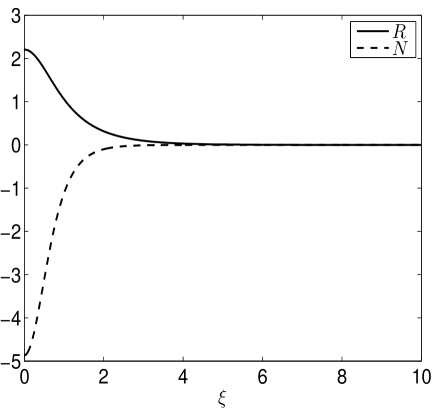
Figure 1: Profiles of the positive solution (ground state) of the equation $\Delta R-R+R^{3}=0$ and of the density $N=-R^{2}$.

At the center of symmetry, $\partial_{\xi}\sigma_{i}$, $\partial_{\xi}\nu_{i}$ and $\upsilon_{i}$ vanish. All the functions also decay at infinity. This leads to the sequence of equations

$$\Delta\sigma_{1}-\sigma_{1}+R^{2}\sigma_{1}-R\nu_{1}=0$$ (41)

$$-\Delta\nu_{1}-2\Delta(R\sigma_{1})={\mathcal{L}}(R^{2})$$ (42)

$$\xi^{-1}\partial_{\xi}(\xi\upsilon_{1})=2R^{2}+\xi(R^{2})_{\xi}$$ (43)

$$\Delta\sigma_{2}-\sigma_{2}+R^{2}\sigma_{2}-R\nu_{2}=-\frac{\xi^{2}}{4}R$$ (44)

$$-\Delta\nu_{2}-2\Delta(R\sigma_{2})=0$$ (45)

$$\Delta\sigma_{3}-\sigma_{3}+R^{2}\sigma_{3}-R\nu_{3}=\Delta^{2}R$$ (46)

$$-\Delta\nu_{3}-2\Delta(R\sigma_{3})=\Delta^{2}(R^{2})$$ (47)

Since the kernel of the operator $\Delta-1+3R^{2}$ is reduced to the null function under a radial symmetry assumption, all the above equations are solvable. We now write that the time evolution of the fields through the variations of the functions $a$, $b$ and $\lambda$ are constrained by the conservation of the plasmon number and of the Hamiltonian that can both be estimated within the above perturbative expansion Malkin (1993).

For the plasmon number, one has (up to a $2\pi$ angular integration factor that we systematically omit)

$${\mathcal{N}}\equiv\int|E|^{2}rdr=$$

$$\quad\int\Big{(}R^{2}+2a^{2}R\sigma_{1}+2bR\sigma_{2}+2\frac{\Gamma}{\lambda^{2}}R\sigma_{3}\Big{)}\xi d\xi+\cdots.$$

(48)

The Hamiltonian reads

$${\mathcal{H}}=\int\Big{(}|\mbox{\boldmath$\nabla$}E|^{2}+n|E|^{2}+\frac{1}{2}n^{2}+\frac{1}{2}V^{2}$$

$$\quad+\Gamma|\Delta E|^{2}+\frac{\Gamma}{2}|\mbox{\boldmath$\nabla$}n|^{2}\Big{)}rdr.$$ (49)

It involves $\displaystyle|{\mbox{\boldmath$\nabla$}E|^{2}=\lambda^{-4}[|\mbox{\boldmath$\nabla$}S|^{2}+(a^{2}\lambda^{2}/4)\xi^{2}S^{2}]}$. Substituting the expansion of the various fields and using that, as already mentioned, the Hamiltonian associated with the ground state solution $(R,-R^{2},0)$ vanishes, one gets

$$\lambda^{2}{\mathcal{H}}=2a^{2}\int(\mbox{\boldmath$\nabla$}R\cdot\mbox{\boldmath$\nabla$}\sigma_{1}-R^{3}\sigma_{1})\xi d\xi$$

$$\qquad+2b\int(\mbox{\boldmath$\nabla$}R\cdot\mbox{\boldmath$\nabla$}\sigma_{2}-R^{3}\sigma_{2})\xi d\xi$$

$$\qquad+\frac{2\Gamma^{2}}{\lambda^{2}}\int\mbox{\boldmath$\nabla$}R\cdot\mbox{\boldmath$\nabla$}\sigma_{3}-R^{3}\sigma_{3})\xi d\xi$$

$$\qquad+\frac{a^{2}\lambda^{2}}{4}\int\xi^{2}R^{2}\xi d\xi+\frac{a^{2}}{2}\int\upsilon_{1}^{2}\xi d\xi$$

$$\qquad+\frac{\Gamma}{\lambda^{2}}\int|\Delta R|^{2}\xi d\xi+\frac{\Gamma}{2\lambda^{2}}\int\big{|}\mbox{\boldmath$\nabla$}(R)^{2}\big{|}^{2}\xi d\xi+\cdots$$

Performing integration by parts in the integrals involving the $\sigma_{i}$’s and using that $R$ obeys $\Delta R-R+R^{3}=0$, one gets

$$\lambda^{2}{\mathcal{H}}=-\int\Big{(}2a^{2}R\sigma_{1}+2bR\sigma_{2}+\frac{2\Gamma}{\lambda^{2}}R\sigma_{3}\Big{)}\xi d\xi$$

$$+\frac{a^{2}\lambda^{2}}{4}\int\xi^{2}R^{2}\xi d\xi+\frac{a^{2}}{2}\int|\upsilon_{1}|^{2}\xi d\xi$$

$$+\frac{\Gamma}{\lambda^{2}}\int\Big{(}|\Delta R|^{2}+\frac{1}{2}\big{|}\mbox{\boldmath$\nabla$}(R^{2})\big{|}^{2}\Big{)}\xi d\xi+\cdots$$ (51)

Using (48), the first integral in the right-hand side of eq. (51) is the difference ${\widetilde{\mathcal{N}}}={\mathcal{N}}-\int R^{2}\xi d\xi$ between the actual plasmon number and its critical value for collapse when $\Gamma=0$. Furthermore, $a^{2}=\lambda_{t}^{2}$. One thus gets the following dynamical equation for the scaling factor $\lambda$

$$\lambda_{t}^{2}=\frac{1}{m_{1}+m_{2}\lambda^{2}}\Big{(}{\mathcal{H}}\lambda^{2}+{\widetilde{\mathcal{N}}}-\frac{\Gamma m_{3}}{\lambda^{2}}\Big{)},$$ (52)

with $m_{1}=(1/2)\int\upsilon^{2}\xi d\xi\approx 0.727$, $m_{2}=(1/4)\int\xi^{2}R^{2}\xi d\xi\approx 0.553$ and $m_{3}=\int\Big{(}|\Delta R|^{2}+(1/2)\big{|}\mbox{\boldmath$\nabla$}(R^{2})\big{|}^{2}\Big{)}\xi d\xi\approx 10.785$ and ${\cal H}<0$. As in Haas and Shukla (2009), the problem can be viewed as the motion of a particle in a potential that diverges positively as $\lambda\to 0$ and has a finite positive limit as $\lambda\to+\infty$. If $\Gamma<{\widetilde{\cal N}}^{2}/4|{\cal H}|m_{3}$, this potential has a negative minimum and $\lambda(t)$ oscillates between strictly positive minimal and maximal values.

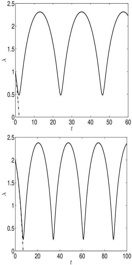
Figure 2: Time variation of the scaling factor $\lambda$ (solid lines) for $\Gamma=5.\ 10^{-3}$, ${\mathcal{H}}=-0.0430$ and ${\widetilde{\mathcal{N}}}=0.240$ (top) and $\Gamma=10^{-3}$, ${\mathcal{H}}=-0.0295$ and ${\widetilde{\mathcal{N}}}=0.168$ (bottom). For comparison, the corresponding evolutions in the case $\Gamma=0$ (dashed lines) are superimposed.

For an explicit numerical resolution, it is more convenient to consider $y=\lambda^{2}$ that obeys

$$y_{t}^{2}=\frac{4}{m_{1}+m_{2}y}\Big{(}{\mathcal{H}}y^{2}+{\widetilde{\mathcal{N}}}y-\Gamma m_{3}\Big{)}$$ (53)

Under the condition $\displaystyle{\Gamma<{\widetilde{\mathcal{N}}^{2}}/\big{(}4\big{|}{\mathcal{H}}\big{|}m_{3}\big{)}}$, there exists positive $y_{m}$ and $y_{M}$ solutions of ${\mathcal{H}}y^{2}+{\widetilde{\mathcal{N}}}y-{\Gamma m_{3}}$ such that $y$ oscillates between $y_{m}=\displaystyle{[{\widetilde{\cal N}}-({\widetilde{\cal N}}^{2}-4{|\cal H|}\Gamma m_{3})^{1/2}]/2{|\cal H|}}$ and $y_{M}=\displaystyle{[{\widetilde{\cal N}}+({\widetilde{\cal N}}^{2}-4{|\cal H|}\Gamma m_{3})^{1/2}]/2{|\cal H|}}$, consistent with the global existence demonstrated in Section III. Equation (53) is equivalently rewritten

$$y_{tt}=\partial_{y}\Big{[}\frac{2}{m_{1}+m_{2}y}\Big{(}{\mathcal{H}}y^{2}+{\widetilde{\mathcal{N}}}y-\Gamma m_{3}\Big{)}\Big{]}.$$ (54)

For a given $y(0)$, one should prescribe

$$y_{t}(0)=-2\left[\frac{{\mathcal{H}}y^{2}(0)+{\widetilde{\mathcal{N}}}y(0)-\Gamma m_{3}}{m_{1}+m_{2}y(0)}\right]^{1/2}.$$ (55)

Figure 2 shows the time evolution of the scaling factor $\lambda(t)$ for $\Gamma=5.\ 10^{-3}$, ${\mathcal{H}}=-0.0430$ and ${\widetilde{\mathcal{N}}}=0.240$ (top) and $\Gamma=10^{-3}$, ${\mathcal{H}}=-0.0295$ and ${\widetilde{\mathcal{N}}}=0.168$ (bottom), corresponding to the initial conditions $E_{0}=2.85\,e^{-r^{2}}$ and $E_{0}=2.90\,e^{-r^{2}}$ respectively, with $n_{0}=-|E_{0}|^{2}$, $V_{0}=0$. For comparison, we superimposed the corresponding evolution when $\Gamma=0$. In this case, $\lambda$ reaches zero in a finite time, with $\lambda_{t}^{2}={\widetilde{N}}/m_{1}=a_{0}^{2}$, consistent with the scaling $\lambda\propto(t_{*}-t)$ of the self-similar blowing-up solutions of the classical Zakharov equations. Note that, while near threshold the two-dimensional scalar model predicts the same leading- order profile for the pump wave as the nonlinear Schrödinger equation resulting from the subsonic approximation (slaved acoustic waves), it does not lead to the same scaling law.

V The two-dimensional electrostatic model

Let us now return to the electrostatic model, first in the case $\Gamma=0$. From eqs. (19)-(20), we perform the rescaling $\displaystyle{\nabla\psi=(1/\lambda){\mathbf{S}}({\mbox{\boldmath$\xi$},\tau)e^{i\tau-ia\lambda{|\mbox{\boldmath$\xi$}|^{2}}/4}}}$, $\displaystyle{n=(1/\lambda^{2})N(\mbox{\boldmath$\xi$},\tau)}$ and $\displaystyle{{\mathbf{v}}=(1/\lambda^{2}){\mathbf{V}}(\mbox{\boldmath$\xi$},\tau)}$. After neglecting as previously the $\tau$-derivatives of the rescaled functions, we get

$$\Delta{\mathbf{S}}-{\mathbf{S}}+b\frac{|\mbox{\boldmath$\xi$}|^{2}}{4}{\mathbf{S}}=$$

$$\qquad e^{ia\lambda{|\mbox{\boldmath$\xi$}|^{2}}/4}\Delta^{-1}\mbox{\boldmath$\nabla$}\Big{(}\mbox{\boldmath$\nabla$}\cdot(N{\mathbf{S}}\,e^{-ia\lambda{|\mbox{\boldmath$\xi$}|^{2}}/4})\Big{)}$$ (56)

$$a^{2}{\cal L}(N)-\Delta N=\Delta|{\mathbf{S}}|^{2}.$$ (57)

The phase factors in eq. (56) introduce a serious difficulty in the sense that their expansions lead to an additional contribution in the perturbative calculation that is not necessarily associated with a well-posed problem, restricting de facto the present analysis to isotropic solutions for which the operator $\Delta^{-1}\,{\rm grad}\,{\rm div}$ reduces to the identity and the phase factors cancel out. Denoting by $S$ the radial component of ${\mathbf{S}}$, one can then perform an analysis similar to that of the scalar model.

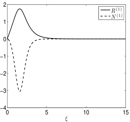
Figure 3: Profiles of the positive solution (ground state) of the equation $\Delta^{(1)}R^{(1)}-R^{(1)}+{R^{(1)}}^{3}=0$ and of the density $N^{(1)}=-{R^{(1)}}^{2}$.

The only difference between the isotropic electrostatic equations and the scalar model is the replacement of the scalar Laplacian in the equation for the electric field by the radial component ${\Delta^{(1)}}$ of the vectorial Laplacian (which implies in particular that the electric field now vanishes at the center of symmetry). Denoting by $R^{(1)}$ the positive solution (fig. 3) of

$$\Delta^{(1)}R^{(1)}-R^{(1)}+{R^{(1)}}^{3}=0$$ (58)

with $R^{(1)}(0)=R^{(1)}(\infty)=0$ (see Fibich and Gavish (2008) for a review on this equation and its extensions that arise in the context of vortex solutions of the nonlinear Schrödinger equation), the rescaled density and velocity satisfy the same equation as in the scalar model, except that $R$ is replaced by $R^{(1)}$. We thus recover eq. (53) with coefficients now given by $m_{1}\approx 24.42$, $m_{2}\approx 8.14$ and $m_{3}\approx 24.94$. Furthermore $\int{R^{(1)}}^{2}\xi d\xi\approx 7.69$. As consequence, the scaling coefficient displays the same oscillatory behavior as in the scalar model.

VI Difficulties in three dimensions

The three-dimensional problem displays specific difficulties even in the context of the scalar model. Indeed, although solutions of the classical scalar model ($\Gamma=0$) with negative Hamiltonian appear to blow up in a self-similar way as in two dimensions, the perturbation analysis for $\Gamma>0$ is not straightforward in three dimensions.

Proceeding as in two dimensions (but with different rescalings), we are looking for solutions of the form $E(r,t)=\lambda^{-3/2}S(\xi,\tau)e^{i(\tau-a\lambda^{1/2}\xi^{2}/4)}$, $n(r,t)=\lambda^{-2}N(\xi,\tau)$, $v(r,t)=\lambda^{-5/2}V(\xi,\tau)$, $n_{t}(r,t)=\lambda^{-7/2}W(\xi,\tau)$, with $\xi=r/\lambda$ with a profile depending only weakly on the rescaled time $\tau$. This leads to

$$\Delta S-S-NS+b\frac{\xi^{2}}{4}S$$

$$\qquad\qquad-\frac{\Gamma}{\lambda^{2}}e^{ia\lambda\xi^{2}/4}\Delta(Se^{-ia\lambda\xi^{2}/4})=0$$ (59)

$$a(\frac{7}{2}W+\xi\partial_{\xi}W)-\lambda\Delta N=\Delta|S|^{2}-\frac{\Gamma}{\lambda}\Delta^{2}N$$ (60)

$$\frac{1}{\xi^{2}}\partial_{\xi}(\xi^{2}\partial_{\xi}V)=-a(2N+\xi\partial_{\xi}N)=-W$$ (61)

$$a(\frac{5}{2}V+\xi\partial_{\xi}V)-\lambda\partial_{\xi}N=-\partial_{\xi}|S|^{2}+\frac{\Gamma}{\lambda}\partial_{\xi}\Delta N$$ (62)

where $a=-\lambda_{t}\lambda^{1/2}=-\lambda_{\tau}\lambda^{-3/2}$ and $b=(a\lambda^{1/2})_{\tau}+(a\lambda^{1/2})^{2}$. From eqs. (61) and (62), we have

$$a^{2}{\mathcal{L}}(N)-\lambda\Delta N=\Delta|S|^{2}-\frac{\Gamma}{\lambda}\Delta^{2}N\\$$ (63)

with now ${\cal L}=\xi^{2}N_{\xi\xi}+(13/2)\xi N_{\xi}+7N$.

In the classical regime ($\Gamma=0$), $a$ has a finite (positive) limit $a_{0}$ as the collapse time is approached, corresponding to a scaling factor varying like $(t_{\star}-t)^{2/3}$. In this regime, the term $\lambda\Delta N$ is negligible in eq. (63) (supersonic regime) and $S$ scales like $a$. However, as shown below, this ordering eventually breaks down in the presence of quantum effects. Indeed, as the collapse is arrested, $\lambda_{t}$ vanishes and so does $a$. This indicates that a systematic modulational theory analogous to what we developed in two dimensions, is not possible in three dimensions. In this context, we resort to limit our address of the problem to a semi-phenomenological approach based on the extension of asymptotic expansions outside their range of strict validity, with the hope to capture qualitative properties of the global dynamics.

For this purpose, we assume that $\Gamma$ is small enough for the quantum effects to start acting only after the system has reached the classical blowing up regime where $a(t)$ is closed to its limit $a_{0}$. In this asymptotic regime, one expects that there exists a period of time during which $a$ remains sufficiently close to $a_{0}$ to allow a perturbative calculation. We are thus led to expand

$$S=a_{0}(S_{0}+bS_{1}+\frac{\lambda}{a_{0}^{2}}S_{2}+\frac{\Gamma}{\lambda^{2}}S_{3}+\frac{\Gamma}{\lambda a_{0}^{2}}S_{4}+\frac{a^{2}-a_{0}^{2}}{a_{0}^{2}}S_{5})$$

$$N=N_{0}+bN_{1}+\frac{\lambda}{a_{0}^{2}}N_{2}+\frac{\Gamma}{\lambda^{2}}N_{3}+\frac{\Gamma}{\lambda a_{0}^{2}}N_{4}+\frac{a^{2}-a_{0}^{2}}{a_{0}^{2}}N_{5}$$

$$V=a_{0}(V_{0}+bV_{1}+\frac{\lambda}{a_{0}^{2}}V_{2}+\frac{\Gamma}{\lambda^{2}}V_{3}+\frac{\Gamma}{\lambda a_{0}^{2}}V_{4}+\frac{a^{2}-a_{0}^{2}}{a_{0}^{2}}V_{5}$$

$$\qquad+(a-a_{0})V_{0}).$$

The lowest order terms $(S_{0},N_{0},V_{0})$ are solutions of

$$\Delta S_{0}-S_{0}-N_{0}S_{0}=0$$ (64)

$${\mathcal{L}}(N_{0})=\Delta(S_{0}^{2})$$ (65)

$$-\xi^{-2}\partial_{\xi}(\xi^{2}V_{0})=2N_{0}+\xi\partial_{\xi}N_{0}.$$ (66)

$$\frac{5}{2}V_{0}+\xi{V_{0}}_{\xi}=-\partial_{\xi}(|S_{0}|^{2})$$ (67)

Their profiles (not shown) are qualitatively very similar to those in two dimensions Landman et al. (1992). The corrections terms $(S_{i},N_{i},V_{i})$ $(i=1,5)$ satisfy the systems

$$\Delta S_{i}-S_{i}-N_{0}S_{i}-S_{0}N_{i}=F_{i}$$ (68)

$${\mathcal{L}}(N_{i})-2\Delta(S_{0}S_{i})=G_{i}$$ (69)

$$\xi^{-2}\partial_{\xi}(\xi^{2}V_{i})=H_{i},$$ (70)

with $F_{1}=-\frac{\xi^{2}}{4}S_{0}$, $G_{1}=0$, $F_{2}=0$, $G_{2}=\Delta N_{0}$, $F_{3}=\Delta^{2}S_{0}$, $G_{3}=0$, $F_{4}=0$, $G_{4}=-\Delta^{2}N_{0}$, $F_{5}=0$, $G_{5}=-{\mathcal{L}}(N_{0})$, and $H_{i}=-a_{0}(2N_{i}+\xi\partial_{\xi}N_{i})$. We find that $S_{5}=\frac{1}{2}S_{0}$ and $N_{5}=V_{5}=0$. The first and last term in the expansion of $S$ thus combine giving $\frac{a^{2}+a_{0}^{2}}{2a_{0}}S_{0}$. Proceeding as in two dimensions, we substitute the expansions of $S,N,V$ into the plasmon number and the Hamiltonian. We get

$${\mathcal{N}}=\alpha_{0}a^{2}+2\alpha_{1}a_{0}^{2}b+2\alpha_{2}\lambda+2\alpha_{3}\Gamma\frac{a_{0}^{2}}{\lambda^{2}}+2\alpha_{4}\frac{\Gamma}{\lambda}+\cdots.$$ (71)

where the coefficients $\alpha_{i}\equiv\int S_{0}S_{i}\xi^{2}d\xi$ are numerically estimated as $\alpha_{0}\approx 1.99$, $\alpha_{1}\approx 1.94$, $\alpha_{2}\approx 0.35$, $\alpha_{3}\approx 51.36$, $\alpha_{4}\approx 34.44$. On the other hand,

$$\lambda^{2}{\mathcal{H}}=\beta_{0}a_{0}^{2}+\beta_{1}a_{0}^{2}a^{2}\lambda+\beta_{2}a_{0}^{2}b+\beta_{3}\lambda+\beta_{4}\Gamma\frac{a_{0}^{2}}{\lambda^{2}}+\beta_{5}\frac{\Gamma}{\lambda}+\cdots$$ (72)

One first proves that

$$\beta_{0}\equiv\int\Big{(}|\mbox{\boldmath$\nabla$}S_{0}|^{2}+n|S_{0}|^{2}+\frac{1}{2}V_{0}^{2}\Big{)}\xi^{2}d\xi=0.$$ (73)

For this purpose, we multiply eq. (64) by $S_{0}$ and by $\xi(S_{0})_{\xi}$ respectively, and integrate in space the resulting equations to get

$$\int(|\mbox{\boldmath$\nabla$}S_{0}|^{2}+N_{0}S_{0}^{2}+S_{0}^{2})\xi^{2}d\xi= 0$$ , (74)

$$\int(|\mbox{\boldmath$\nabla$}S_{0}|^{2}+3N_{0}S_{0}^{2}+3S_{0}^{2}+\xi{N_{0}}_{\xi}S_{0}^{2})\xi^{2}d\xi= 0$$ . (75)

Subtracting these two equalities and using (66), we have

$$\int[2S_{0}^{2}+V_{0}\partial_{\xi}(S_{0}^{2})]\xi^{2}d\xi=0.$$ (76)

Multiplying (67) by $V_{0}$ and integrating in space, we get

$$\int V_{0}^{2}\xi^{2}d\xi=-\int(S_{0}^{2})_{\xi}V_{0}\xi^{2}d\xi.$$ (77)

Combining (76) and (77) gives $\int S_{0}^{2}\xi^{2}d\xi=\frac{1}{2}\int V_{0}^{2}\xi^{2}d\xi$, which after substitution in (74) leads to (73).

Using eqs. (64)-(70), the constants $\beta_{i}$ for $i=1,\cdots 5$ are given by $\beta_{1}=\int\frac{\xi^{2}}{4}S_{0}^{2}\approx 1.17$, $\beta_{2}=\int(\frac{\xi^{2}}{4}S_{0}^{2}-2S_{0}S_{1}+V_{0}V_{1})\xi^{2}d\xi\approx-1.17$, $\beta_{3}=\int(-2S_{0}S_{2}+V_{0}V_{2}+\frac{1}{2}N_{0}^{2})\xi^{2}d\xi\approx 3.10$, $\beta_{4}=\int(-2S_{0}S_{3}+V_{0}V_{3})\xi^{2}d\xi\approx-5.56$, $\beta_{5}=\int(-2S_{0}S_{4}+V_{0}V_{4}+\frac{1}{2}|\mbox{\boldmath$\nabla$}N_{0}|^{2})\xi^{2}d\xi\approx-2.81$.

We now eliminate the term proportional to $a^{2}b$ in ${\mathcal{H}}$ using ${\mathcal{N}}$ and find

$$\lambda^{2}{\mathcal{H}}=m_{1}a_{0}^{2}a^{2}\lambda+m_{2}\lambda+m_{3}\Gamma\frac{a_{0}^{2}}{\lambda^{2}}+m_{4}a^{2}$$

$$\quad+m_{5}\frac{\Gamma}{\lambda}+m_{6}{\cal N}.$$ (78)

The new constants $m_{i}$ are defined as $m_{1}=\beta_{1}\approx 1.17$, $m_{2}=\beta_{3}-\alpha_{2}\beta_{2}/\alpha_{1}\approx 3.31$, $m_{3}=\beta_{4}-\alpha_{3}\beta_{2}/\alpha_{1}\approx 25.41$, $m_{4}=-\alpha_{0}\beta_{2}/(2\alpha_{1})\approx 0.60$, $m_{5}=\beta_{5}-\alpha_{4}\beta_{2}/\alpha_{1}\approx 17.95$, $m_{6}=\beta_{2}/(2\alpha_{1})\approx-0.30$.

Inserting that $a=-\lambda_{t}\lambda^{1/2}$, the effective ODE satisfied by $\lambda$ is

$$\lambda_{t}^{2}=-\frac{m_{2}\lambda^{3}+m_{3}\Gamma a_{0}^{2}+m_{5}\Gamma\lambda+m_{6}{\mathcal{N}}\lambda^{2}-{\mathcal{H}}\lambda^{4}}{\lambda^{2}(m_{1}a_{0}^{2}\lambda^{2}+m_{4}\lambda)}$$ (79)

In order to fix the parameter $a_{0}$, we note that for $\Gamma=0$, in the blowing up regime where $\lambda\to 0$, one has

$$a_{0}^{2}=\lim_{\lambda\to 0}a^{2}=\lim_{\lambda\to 0}\lambda_{t}^{2}\lambda=-\frac{m_{6}{\mathcal{N}}}{m_{4}},$$ (80)

or using the definitions of $m_{4}$ and $m_{6}$,

$$a_{0}^{2}=\frac{\mathcal{N}}{\int S_{0}^{2}\xi^{2}d\xi}.$$ (81)

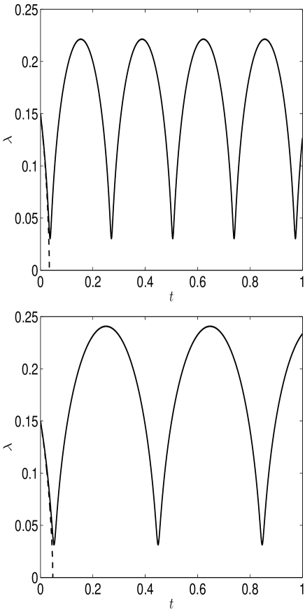
Figure 4: Time variation of the scaling factor $\lambda$ for the three-dimensional phenomenological model, when ${\mathcal{N}}=5.64$ and ${\mathcal{H}}=-18.97$, with $\Gamma=2.\ 10^{-5}$ (top) and ${\mathcal{N}}=2.76$ and ${\mathcal{H}}=-0.33$, with the sale value of $\Gamma$ as above. For comparison, the corresponding evolutions in the case $\Gamma=0$ (dashed lines) are superimposed.

Figure 4 (top) shows the evolution of the scaling factor $\lambda(t)$ for ${\mathcal{N}}=5.64$ and ${\mathcal{H}}=-18.97$ (corresponding to an initial conditions $E_{0}=ce^{-r^{2}}$, $n_{0}=-|E_{0}|^{2}$, and $v_{0}=0$ with $c=6$, for the original Zakharov equations) and $\Gamma=2.\ 10^{-5}$. For comparison, the evolution in the absence of quantum effects is also displayed. As in two dimensions, we observe that quantum effects induce a periodic behavior. In simulations with smaller $\Gamma$, the minimum of $\lambda$ is, as expected, getting smaller. When keeping the same value of $\Gamma$, one uses ${\mathcal{H}}=-0.32$ with ${\mathcal{N}}=2.76$ by taking $c=4.2$, the maximum of $\lambda$ is slightly increased, while the period of the oscillation gets significantly longer (Fig. 4 bottom), but the global behavior remains very similar. Note however that the dynamics is much faster than in two dimensions. This effect is already visible on the singularity time at $\Gamma=0$, a regime for which eq. (79) is asymptotically exact. This suggests that the parameters we used in three dimensions (even for the bottom panel of Fig. 4) correspond to a regime significantly distant from the threshold conditions that in this case are not as easily characterized as in two dimensions. As stressed at the beginning of this section, the present description of the three-dimensional problem is however to be viewed as heuristic, as the asymptotics clearly breaks down before the scaling factor $\lambda(t)$ reaches its minimum. It nevertheless predicts a behavior consistent with the arrest of collapse (the proof given in Section I is easily transposed to the scalar model). It also shows a periodic dynamics whose origin is expected to be generic. It indeed results from a competition between wave focusing that occurs when $\lambda$ is not yet small enough for the quantum effects to act efficiently, and the subsequent evolution that takes place when the influence of the latter perturbations dominates the dynamics and leads to defocusing until the moment where, $\lambda$ becoming large enough, their influence becomes again subdominant, thus permitting an efficient self-focusing. Validation of the model would require comparisons with direct simulations of the scalar model, an issue that is outside the scope of the present paper. Compared with the Rayleigh-Ritz method, the present approach should provide a better description of the solution profile. It also more clearly points out the conditions of applicability of modulation methods.

VII Conclusion

The influence of quantum effects on the Langmuir wave dynamics provides an interesting example of the action of an additional dispersive effect on the phenomenon of wave collapse, although in realistic situations the Zakharov description is supposed to break down before quantum effects become relevant. Arrest of collapse was predicted Haas and Shukla (2009) in the adiabatic regime where the density is slaved to the wave amplitude, using a Rayleigh Ritz method. Here, the result is rigorously established for the full quantum Zakharov equations, by combining the conservation of the plasmon number and of the Hamiltonian with estimates based on a Gagliardo-Nirenberg inequality. These invariances are also used to develop a systematic perturbative expansion in order to capture the influence of weak quantum effects for initial conditions slightly above the singularity threshold for the classical problem. Restricted for technical reasons to isotropic solutions (at least in the focusing region), the analysis is carried out in two space dimensions corresponding to the critical dimension for collapse of the cubic nonlinear Schrödinger equation. The difficulty of extending the analysis to three dimensions points out the importance of the proximity of criticality to satisfy the delicate balances involved in a systematic asymptotic theory. We thus resorted in this case to develop a semi-phenomenological approach.

References

• Zakharov (1972) V. E. Zakharov, Sov. Phys. JETP 35, 908 (1972).
• Garcia et al. (2005) L. G. Garcia, F. Haas, L. P. L. de Oliveira, and J. Goedert, Phys. Plasmas 12, 012302 (2005).
• Haas and Shukla (2009) F. Haas and P. K. Shukla, Phys. Rev. E 79, 066402 (2009).
• Kuznetsov (1974) E. A. Kuznetsov, Sov. Phys. JETP 39, 1003 (1974).
• Sulem and Sulem (1979) C. Sulem and P.-L. Sulem, C.R. Acad. Sci. Paris 289 A, 173 (1979).
• Added and Added (1984) H. Added and S. Added, C.R. Acad. Sci. Paris A 299, 551 (1984).
• Glangletas and Merle (1994a) L. Glangletas and F. Merle, Comm. Math. Phys. 160, 349 (1994a).
• Ginibre et al. (1997) J. Ginibre, Y. Tsutsumi, and G. Velo, J. Funct. Anal. 151, 384 (1997).
• Sulem and Sulem (1999) C. Sulem and P. L. Sulem, The Nonlinear Schrödinger equation: Self-focusing and wave collapse, Applied Mathematical Sciences 139 (Springer, 1999).
• Degtyarev and Kopa-Ovdienko (1984) L. M. Degtyarev and A. L. Kopa-Ovdienko, Sov. J. Plasma Phys. 10, 3 (1984).
• Adams (1978) R. Adams, Sobolev spaces (Academic Press, 1978).
• Cazenave (2003) T. Cazenave, Semilinear Schrödinger equations, Courant Lectures Notes (American Mathematical Society, 2003).
• Weinstein (1983) M. I. Weinstein, Comm. Math. Phys. 87, 567 (1983).
• Agueh (2008) M. Agueh, C.R. Acad. Sci. Paris, Ser. I 346, 757 (2008).
• Galusinski (2000) C. Galusinski, M2AN 34, 109 (2000).
• Papanicolaou et al. (1991) C. G. Papanicolaou, C. Sulem, P. L. Sulem, and X. P. Wang, Phys. Fluids B 3, 969 (1991).
• Malkin (1993) V. Malkin, Physica D 64, 251 (1993).
• Fibich and Papanicolaou (1999) G. Fibich and G. C. Papanicolaou, SIAM J. Appl. Math. 60, 183 (1999).
• Landman et al. (1992) M. J. Landman, C. G. Papanicolaou, C. Sulem, P. L. Sulem, and X. P. Wang, Phys. Rev. A 46, 7869 (1992).
• Fibich and Gavish (2008) G. Fibich and N. Gavish, Physica D 237, 2696 (2008).
• Karpman and Shagalov (2000) V. I. Karpman and A. Shagalov, Physica D 144, 194 (2000).
• Fibich et al. (2002) G. Fibich, B. Ilan, and G. Papanicolaou, SIAM J. Appl. Math. 62, 1437 (2002).
• Bourgain and Colliander (1996) J. Bourgain and J. Colliander, Intern.Math. Res. Notices 11, 515 (1996).
• Bejenaru et al. (2009) I. Bejenaru, S. Herr, J. Holmer, and D. Tataru, Nonlinearity 22, 1063 (2009).
• Gidas et al. (1981) B. Gidas, W. M. Ni, and L. Nirenberg, Adv. Math. Supp. Studies 7A, 369 (1981).
• Glangletas and Merle (1994b) L. Glangletas and F. Merle, Comm. Math. Phys. 160, 173 (1994b).