Scaling Analysis of Affinity Propagation

Abstract

We analyze and exploit some scaling properties of the Affinity Propagation (AP) clustering algorithm proposed by Frey and Dueck (2007). First we observe that a divide and conquer strategy, used on a large data set hierarchically reduces the complexity ${\cal O}(N^{2})$ to ${\cal O}(N^{(h+2)/(h+1)})$, for a data-set of size $N$ and a depth $h$ of the hierarchical strategy. For a data-set embedded in a $d$-dimensional space, we show that this is obtained without notably damaging the precision except in dimension $d=2$. In fact, for $d$ larger than $2$ the relative loss in precision scales like $N^{(2-d)/(h+1)d}$. Finally, under some conditions we observe that there is a value $s^{*}$ of the penalty coefficient, a free parameter used to fix the number of clusters, which separates a fragmentation phase (for $s<s^{*}$) from a coalescent one (for $s>s^{*}$) of the underlying hidden cluster structure. At this precise point holds a self-similarity property which can be exploited by the hierarchical strategy to actually locate its position. From this observation, a strategy based on AP can be defined to find out how many clusters are present in a given dataset.

1 Introduction

Since its invention by J. Pearl [1] in the context of Bayesian inference, it has been realized that the belief-propagation algorithm was related to many other algorithms encountered in various fields [2] and it has since diffused in many different areas (inference problems, signal processing, error codes, image segmentation …). In the context of statistical physics, it is closely related to a certain type of mean-field approach (Bethe-Peierls), more precisely the so-called Bethe-approximation, valid on sparse graphs [3]. This reconsideration in statistical physics terms, has given rise to a new generation of distributed algorithms. These address NP-hard combinatorial optimization problems, like the survey-propagation algorithm of Mézard and Zecchina [4] for the random K-SAT problems, where the factor-graph has a tree-like structure. Surprisingly enough, in some other context it works also well on dense factor-graphs as exemplified by the affinity propagation algorithm proposed by Frey and Dueck [5] for the clustering problem, which is also NP-hard. Akin $K$-centers, AP maps each data item onto an actual data item, called exemplar, and all items mapped onto the same exemplar form one cluster. Contrasting with $K$-centers, AP builds quasi-optimal clusters in terms of distortion, thus enforcing the cluster stability [5]. The price to pay for these understandability and stability properties is a quadratic computational complexity, except if the similarity matrix is made sparse with help of a pruning procedure. Nevertheless, a pre-treatment of the data would also be quadratic in the number if item, which is severely hindering the usage of AP on large scale datasets. The basic assumption behind AP, is that cluster are of spherical shape. This limiting assumption has actually been addressed by Leone and co-authors in [6, 7], by softening a hard constraint present in AP, which impose that any exemplar has first to point to itself as oneself exemplar. Another drawback, which is actually common to most clustering techniques, is that there is a free parameter to fix which ultimately determines the number of clusters. Some methods based on EM [8, 9] or on information-theoretic consideration have been proposed[10], but mainly use a precise parametrization of the cluster model. There exist also a different strategy based on similarity statistics [11], that have been already recently combined with AP [12], at the expense of a quadratic price. In an earlier work [13, 14], a hierarchical approach, based on a divide and conquer strategy was proposed to decrease the AP complexity and adapt AP to the context of Data Streaming. In this paper we extend the scaling analysis of this procedure initiated in [14] and propose a way to determine the number of clusters.

The paper is organized as follows.In Section 2 we start from a brief description of BP and some of its properties. We see how AP can be derived from it and present some extensions to AP, including the soft-constraint affinity propagation extension (SCAP) to AP. In Section 3, the computational complexity of Hi-AP  is analyzed and the leading behavior, of the resulting error measured on the distribution of exemplars, which depends on the dimension and on the size of the subsets, is computed. Based on these results we enforce the self-similarity of Hi-AP in Section 4 to develop a renormalized version of AP (in the statistical physics sense). We finally discuss how to fix in a self-consistent way the penalty coefficient present in AP, which is conjugate to the number of cluster.

2 Introduction to belief-propagation

2.1 Local marginal computation

The belief propagation algorithm is intended to computing marginals of joint-probability measure of the type

$$P({\bf x})=\prod_{a}\psi_{a}(x_{a})\prod_{i}\phi(x_{i}),$$ (2.1)

where ${\bf x}=(x_{1},\ldots,x_{N})$ is a set of variables, $x_{a}=\{x_{i},i\in a\}$ a subset of variables involved in the factor $\psi_{a}$, while the $\phi_{i}$’s are single variable factors. The structure of the joint measure $P_{a}$ is conveniently represented by a factor graph [2], i.e. a bipartite graph with two set of vertices, $\cal F$ associated to the factors, and $\cal V$ associated to the variables, and a set of edges $\cal E$ connecting the variables to their factors (see Figure 2.1. Computing the single variables marginals scales in general exponentially with the size of the system, except when the underlying factor graph has a tree like structure. In that case all the single site marginals may be computed at once, by solving the following iterative scheme due to J. Pearl [1]:

$$m_{a\to i}(x_{i}) \longleftarrow\sum_{x_{j}\atop j\in a,j\neq i}\psi_{a}(x_{a})\prod_{j}n_{j\to a}(x_{j})$$

$$n_{i\to a}(x_{i}) \longleftarrow\phi_{i}(x_{i})\prod_{b\ni i,b\neq a}m_{b\to i}(x_{i}).$$

$m_{a\to i}(x_{i})$ is called the message sent by factor node $a$ to variable node $i$, while $n_{i\to a}(x_{i})$ is the message sent by variable node $i$ to $a$. These quantities would actually appear as intermediate computations terms, while deconditioning (2.1). On a singly connected factor graph, starting from the leaves, two sweeps are sufficient to obtain the fixed points messages, and the beliefs (the local marginals) are then obtained from these sets of messages using the formulas:

$$b(x_{i}) =\frac{1}{Z_{i}}\phi_{i}(x_{i})\prod_{a\ni i}m_{a\to i}(x_{i})$$

$$b_{a}(x_{a}) =\frac{1}{Z_{a}}\psi_{a}(x_{a})\prod_{i\in a}n_{i\to a}(x_{i})$$

On a multiply connected graph, this scheme can be used as an approximate procedure to compute the marginals, still reliable on sparse factor graph, while avoiding the exponential complexity of an exact procedure. Many connections with mean field approaches of statistical physics have been recently unravelled, in particular the connection with the TAP equations introduced in the context of spin glasses [15], and the Bethe approximation of the free energy which we detail now.

Figure 2.1: Example of a factor-graph representing a joint measure of five variables (circles) and three factors (squares)

2.2 AP and SCAP as min-sum algorithms

The AP algorithm is a message-passing procedure proposed by Frey and Dueck [5] that performs a classification by identifying exemplars. It solves the following optimization problem

$${\bf c}^{*}=\operatorname*{\text{argmin}}\bigl{(}E[{\bf c}]\bigr{)},$$

with

$$E[{\bf c}]\stackrel{{\scriptstyle\mbox{\tiny def}}}{{=}}-\sum_{i=1}^{N}S(i,c_{i})-\sum_{\mu=1}^{N}\log\chi_{\mu}[{\bf c}]$$ (2.2)

where ${\bf c}=(c_{1},\ldots,c_{N})$ is the mapping between data and exemplars, $S(i,c_{i})$ is the similarity function between $i$ and its exemplar. For datapoints embedded in an Euclidean space, the common choice for $S$ is the negative squared Euclidean distance. A free positive parameter is given by

$$s\stackrel{{\scriptstyle\mbox{\tiny def}}}{{=}}-S(i,i),\qquad\forall i,$$

the penalty for being oneself exemplar. $\chi_{\mu}^{(p)}[{\bf c}]$ is a set of constraints. They read

$$\chi_{\mu}[{\bf c}]=\begin{cases}p,\qquad\text{if}\ c_{\mu}\neq\mu,\exists i\ s.t.\ c_{i}=\mu,\\[5.69046pt] 1,\qquad\text{otherwise}.\end{cases}$$

$p=0$ is the constraint of the model of Frey-Dueck. Note that this strong constraint is well adapted to well-balanced clusters, but probably not to ring-shape ones. For this reason Leone et. al. [6, 7] have introduced the smoothing parameter $p$. Introducing the inverse temperature $\beta$,

$$P[{\bf c}]\stackrel{{\scriptstyle\mbox{\tiny def}}}{{=}}\frac{1}{Z}\exp(-\beta E[{\bf c}])$$

represents a probability distribution over clustering assignments $c$. At finite $\beta$ the classification problem reads

$${\bf c}^{*}=\operatorname*{\text{argmax}}\bigl{(}P[{\bf c}]\bigr{)}.$$

The AP or SCAP equations can be obtained from the standard BP equation [5, 6] as an instance of the Max-Product algorithm. For self-containess, let us reproduce the derivation here. The BP algorithm provides an approximate procedure to the evaluation of the set of single marginal probabilities $\{P_{i}(c_{i}=\mu)\}$ while the min-sum version obtained after taking $\beta\to\infty$ yields the affinity propagation algorithm of Frey and Dueck.

Figure 2.2: Factor graph corresponding to AP. Small squares represents the constraints while large ones are associated to pairwise contributions in the $E({\bf c})$.

The factor-graph involves variable nodes $\{i,i=1\ldots N\}$ with corresponding variable $c_{i}$ and factor nodes $\{\mu,\mu=1\ldots N\}$ corresponding to the energy terms and to the constraints (see Figure 2.2). Let $A_{\mu\to i}(c_{i})$ the message sent by factor $\mu$ to variable $i$ and $B_{i\to\mu}(c_{i})$ the message sent by variable $i$ to node $\mu$. The belief propagation fixed point equations read:

$$A_{\mu\to i}(c_{i}=c) =\frac{1}{Z_{\mu\to i}}\sum_{\{c_{j}\}}\prod_{j\neq i}B_{j\to\mu}(c_{j})\chi_{\mu}^{\beta}[\{c_{j}\},c]$$ (2.3)

$$B_{i\to\mu}(c_{i}=c) =\frac{1}{Z_{i\to\mu}}\prod_{\nu\neq\mu}A_{\nu\to i}(c)e^{\beta S(i,c)}$$ (2.4)

Once this scheme has converged, the fixed points messages provide a consistency relationship between the two sets of beliefs

$$b_{\mu}[\{c_{i}\}={\bf c}] =\frac{1}{Z_{\mu}}\chi_{\mu}^{\beta}[{\bf c}]\prod_{i=1}^{N}B_{i\to\mu}(c_{i})$$ (2.5)

$$b_{i}(c_{i}=c) =\frac{1}{Z_{i}}\prod_{\mu=1}^{N}A_{\mu\to i}[c]e^{\beta S(i,c)}$$ (2.6)

The joint probability measure then rewrites

$$P[{\bf c}]=\frac{1}{Z_{b}}\frac{\prod_{\mu=1}^{N}b_{\mu}[{\bf c}]}{\prod_{i=1}^{N}b_{i}^{N-1}(c_{i})}$$

with $Z_{b}$ the normalization constant associated to this set of beliefs. In (2.3) we observe first that

$$\hat{A}_{\mu\to i}\stackrel{{\scriptstyle\mbox{\tiny def}}}{{=}}A_{\mu\to i}(c_{i}=\nu\neq\mu),$$ (2.7)

is independent of $\nu$ and secondly that $A_{\mu\to i}(c_{i}=c)$ depends only on $B_{j\to\mu}(c_{j}=\mu)$ and on $\sum_{\nu\neq\mu}B_{j\to\mu}(c_{j}=\nu)$. This means that the scheme can be reduced to the propagation of four quantities, by letting

$$A_{\mu\to i} \stackrel{{\scriptstyle\mbox{\tiny def}}}{{=}}A_{\mu\to i}(c_{i}=\mu),$$

$$\hat{A}_{\mu\to i} \stackrel{{\scriptstyle\mbox{\tiny def}}}{{=}}\frac{1-A_{\mu\to i}}{N-1}$$

$$B_{i\to\mu} \stackrel{{\scriptstyle\mbox{\tiny def}}}{{=}}B_{i\to\mu}(c_{i}=\mu)$$

$$\bar{B}_{i\to\mu} \stackrel{{\scriptstyle\mbox{\tiny def}}}{{=}}1-B_{i\to\mu},$$

which reduce to two types of messages $A_{\mu\to i}$ and $B_{i\to\mu}$. The belief propagation equations reduce to

$$A_{\mu\to i} =\frac{p+(1-p)B_{\mu\to\mu}}{p+(1-p)B_{\mu\to\mu}+(N-1)\Bigl{[}p+(1-p)\bigl{(}B_{\mu\to\mu}+\prod_{j\neq i}\bar{B}_{j\to\mu}\bigr{)}\Bigr{]}},\qquad\mu\neq i$$

$$A_{i\to i} =\frac{1}{1+(N-1)\Bigl{[}p+(1-p)\prod_{j\neq i}\bar{B}_{j\to i}\Bigr{]}},$$

$$B_{i\to\mu} =\frac{1}{1+(N-1)\sum_{\nu\neq\mu}\frac{A_{\nu\to i}}{\hat{A}_{\nu\to i}}e^{\beta(S(i,\nu)-S(i,\mu))}},$$

while the approximate single variable belief reads

$$P_{i}(c_{i}=\mu)=\frac{1}{Z_{i}}\ \frac{A_{\mu\to i}}{\hat{A}_{\mu\to i}}\ e^{\beta S(i,\mu)}.$$

This simplification here is actually the key-point in the effectiveness of AP, because this let the complexity of this algorithm, which was potentially $N^{N}$ becomes $N^{2}$, as will be more obvious later. At this point we introduce the log-probability ratios,

$$a_{\mu\to i} \stackrel{{\scriptstyle\mbox{\tiny def}}}{{=}}\frac{1}{\beta}\log\Bigl{(}\frac{A_{\mu\to i}}{\hat{A}_{\mu\to i}}\Bigr{)},$$

$$r_{i\to\mu} \stackrel{{\scriptstyle\mbox{\tiny def}}}{{=}}\frac{1}{\beta}\log\Bigl{(}\frac{B_{i\to\mu}}{\bar{B}_{i\to\mu}}\Bigr{)},$$

corresponding respectively to the “availability” and “responsibility” messages of Frey-Dueck. At finite $\beta$ the equation reads

$$e^{\beta a_{\mu\to i}} =\frac{e^{-\beta q}+(1-e^{-\beta q})e^{\beta r_{\mu\to\mu}}}{e^{-\beta q}+e^{\beta r_{\mu\to\mu}}+(1-e^{-\beta q})\bigl{(}1+e^{\beta r_{\mu\to\mu}}\bigr{)}\prod_{j\neq i}\bigl{(}1+e^{\beta r_{j\to\mu}}\bigr{)}^{-1}}$$

$$e^{-\beta a_{i\to i}} =e^{-\beta q}+(1-e^{-\beta q})\prod_{j\neq i}\bigl{(}1+e^{\beta r_{j\to i}}\bigr{)}^{-1}$$

$$e^{-\beta r_{i\to\mu}} =\sum_{\nu\neq\mu}e^{-\beta\bigl{(}S(i,\mu)-a_{\nu\to i}-S(i,\nu)\bigr{)}},$$

with $q\stackrel{{\scriptstyle\mbox{\tiny def}}}{{=}}-\frac{1}{\beta}\log p$. Taking the limit $\beta\to\infty$ at fixed $q$ yields

$$a_{\mu\to i} =\min\Bigl{(}0,\max\bigl{(}-q,\min(0,r_{\mu\to\mu})\bigr{)}+\sum_{j\neq i}\max(0,r_{j\to\mu})\Bigr{)},\qquad\mu\neq i,$$ (2.8)

$$a_{i\to i} =\min\Bigl{(}q,\sum_{j\neq i}\max(0,r_{j\to i})\Bigr{)},$$ (2.9)

$$r_{i\to\mu} =S(i,\mu)-\max_{\nu\neq\mu}\bigl{(}a_{\nu\to i}+S(i,\nu)\bigr{)}.$$ (2.10)

After reaching a fixed point, exemplars are obtained according to

$$c_{i}^{*}=\operatorname*{\text{argmax}}_{\mu}\bigl{(}S(i,\mu)+a_{\mu\to i}\bigr{)}=\operatorname*{\text{argmax}}_{\mu}\bigl{(}r_{i\to\mu}+a_{\mu\to i}\bigr{)}.$$ (2.11)

Altogether, 2.8,2.9,2.10 and 2.11 constitute the equations of SCAP which reduce to the equations of AP when $q$ tends to $-\infty$.

3 Hierarchical affinity propagation (Hi-AP)

3.1 Weighted affinity propagation (WAP)

Assume that a subset ${\cal S}\subset{\cal E}$ of $n$ points, assumed to be at a small average mutual distance $\epsilon$ are aggregated into a single point $c\in{\cal S}$. The similarity matrix has to be modified as follows

$$S(c,i) \longrightarrow nS(c,j),\qquad\qquad\forall i\in\bar{\cal S}$$

$$S(i,c) \longrightarrow S(i,c),\qquad\qquad\ \ \forall i\in\bar{\cal S}$$

$$S(c,c) \longrightarrow\sum_{i\in{\cal S}}S(i,c),$$

and all lines and columns with index $i\in{\cal S}\backslash\{c\}$ are suppressed from the similarity matrix. This type of rules should be applied when performing hierarchies.

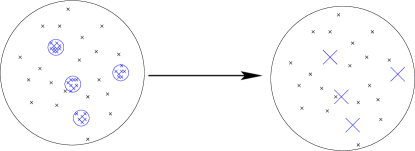
Figure 3.3:

This redefinition of the self-similarity yields a non-uniform penalty coefficient. In the basic update equations (2.8), (2.9), (2.10) and (2.11), nothing prevents from having different self-similarities because while the key property (2.7) for deriving these equations is not affected by this. When comparing in (2.2), the relative contribution of the similarities between different points on one hand, and the penalties on the other hand, we immediately see that $s$ has to scale like the size of the dataset. This insures a basic scale invariance of the result, i.e. that the same solution is recovered, when the number of points in the dataset is rescaled by some arbitrary factor. Now, if we deal directly with weighted data points in an Euclidean space, the preceding considerations suggests that one may start directly from the following rescaled cost function:

$$E[{\bf c}]\stackrel{{\scriptstyle\mbox{\tiny def}}}{{=}}\frac{1}{Z}\sum_{c=1}^{n}\sum_{i\in c}\bigl{(}w_{i}d^{2}(i,c)+\frac{n}{V}s\bigr{)}.$$ (3.1)

$Z$ is a normalization constant

$$Z\stackrel{{\scriptstyle\mbox{\tiny def}}}{{=}}\sum_{i\in{\cal S}}w_{i},$$

The similarity measure has been specified with help of the Euclidean distance

$$d(i,j)=|{\mbox{\bf r}}_{i}-{\mbox{\bf r}}_{j}|,\qquad\qquad\forall(i,j)\in{\cal S}^{2}.$$

The $\{w_{i},\forall i\in{\cal S}\}$ is a set of weights attached to each datapoint and the self-similarity has been rescaled uniformly

$$s\longrightarrow\frac{1}{V}\sum_{i\in{\cal S}}w_{i}\ s.$$

with respect to density of the dataset, $V$ being the volume of the embedding space, for later purpose (thermodynamic limit in Section 4).

3.2 Complexity of Hi-AP

AP computational complexity is expected to scale like ${\cal O}(N^{2})$; it involves the matrix $S$ of pair distances, with quadratic complexity in the number $N$ of items, severely hindering its use on large-scale datasets.

This AP limitation can be overcome through a Divide-and-Conquer heuristics inspired from [17]. Dataset $\cal E$ is randomly split into $b$ data subsets as shown on Figure 3.4; AP is launched on every subset and outputs a set of exemplars; the exemplar weight is set to the number of initial samples it represents; finally, all weighted exemplars are gathered and clustered using WAP (the complexity is ${\cal O}(N^{3/2})$ [13]). This Divide-and-Conquer strategy $-$ which could actually be combined with any other basic clustering algorithm $-$ can be pursued hierarchically in a self-similar way, as a branching process with $b$ representing the branching coefficient of the procedure, defining the Hierarchical AP (Hi-AP) algorithm.

Figure 3.4:

Formally, let us define a tree of clustering operations, where the number $h$ of successive random partitions of the data represents the height of the tree. At each level of the hierarchy, the penalty parameter $s_{*}$ is set such that the expected number of exemplars extracted along each clustering step is upper bounded by some constant $K$.

Proposition 3.1.

Letting the branching factor $b$ to

$$b=\bigl{(}\frac{N}{K}\bigr{)}^{\frac{1}{h+1}},$$

then the overall complexity $C(h)$ of Hi-AP  is given by

$$C(h)\propto K^{\frac{h}{h+1}}N^{\frac{h+2}{h+1}}\qquad N\gg K.$$

Proof.

$M=N/b^{h}$ is the size of each subset to be clustered at level $h$; at level $h-1$, each clustering problem thus involves $bK=M$ exemplars with corresponding complexity

$$C(0)=K^{2}\bigl{(}\frac{N}{K}\bigr{)}^{\frac{2}{h+1}}.$$

The total number $N_{cp}$ of clustering procedures involved is

$$N_{cp}=\sum_{i=0}^{h}b^{i}=\frac{b^{h+1}-1}{b-1},$$

with overall computational complexity:

$$C(h)=K^{2}\bigl{(}\frac{N}{K}\bigr{)}^{\frac{2}{h+1}}\frac{\frac{N}{K}-1}{\bigl{(}\frac{N}{K}\bigr{)}^{\frac{1}{h+1}}-1}\operatorname*{\approx}_{N\gg K}K^{2}\bigl{(}\frac{N}{K}\bigr{)}^{\frac{h+2}{h+1}}.$$

It is seen that $C(0)=N^{2}$, $C(1)\propto N^{3/2}$,…, and $C(h)\propto N$ for ${h\gg 1}$ .  

3.3 Information loss of Hi-AP

Let us examine the price to pay for this complexity reduction. As mentioned earlier on, the clustering quality is usually assessed from its distortion, the sum of the squared distance between every data item and its exemplar:

$$D({\mbox{\bf c}})=\sum_{i=1}^{N}d^{2}(e_{i},c_{i})$$

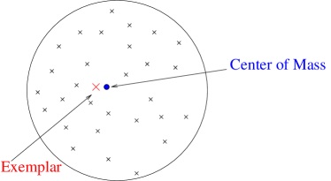
Figure 3.5:

The information loss incurred by Hi-AP w.r.t. AP is examined in the simple case where the data samples follow a centered distribution in ${\rm IR}^{d}$. By construction, AP aims at finding the cluster exemplar r${}_{{\mbox{\bf c}}}$ nearest to the center of mass of the sample points noted ${\mbox{\bf r}}_{cm}$:

$$D({\mbox{\bf c}})=|{\mbox{${\mbox{\bf r}}_{cm}$}}\ -{\mbox{\bf r${}_{{\mbox{\bf c}}}$}}|^{2}+Cst$$

To assess the information loss incurred by Hi-AP it turns out to be more convenient to compare the results in distribution. This can be done by considering e.g. the relative entropy, or Kullback Leibler distance, between the distribution $P_{{\mbox{\bf c}}}$ of the cluster exemplar computed by AP, and the distribution $P_{{\mbox{\bf c}}(h)}$ of the cluster exemplar computed by Hi-AP with hierarchy-depth $h$:

$$D_{KL}\bigl{(}\mbox{$P_{{\mbox{\bf c}}}$}||\mbox{$P_{{\mbox{\bf c}}(h)}$}\bigr{)}=\int\mbox{$P_{{\mbox{\bf c}}(h)}$}(r)\log\frac{\mbox{$P_{{\mbox{\bf c}}(h)}$}(r)}{\mbox{$P_{{\mbox{\bf c}}}$}(r)}d{\bf r}$$ (3.2)

In the simple case where points are sampled along a centered distribution in ${\rm IR}^{d}$, let $\tilde{\mbox{\bf r}}_{{\mbox{\bf c}}}$ denote the relative position of exemplar r${}_{{\mbox{\bf c}}}$ with respect to the center of mass ${\mbox{\bf r}}_{cm}$:

$${\mbox{$\tilde{\mbox{\bf r}}_{{\mbox{\bf c}}}$}}={\mbox{\bf r${}_{{\mbox{\bf c}}}$}}-{\mbox{${\mbox{\bf r}}_{cm}$}}$$

The probability distribution of $\tilde{\mbox{\bf r}}_{{\mbox{\bf c}}}$ conditionally to ${\mbox{\bf r}}_{cm}$ is cylindrical; the cylinder axis supports the segment (0, ${\mbox{\bf r}}_{cm}$), where $0$ is the origin of the $d$-dimensional space. As a result, the probability distribution of ${\mbox{\bf r}}_{cm}$+ $\tilde{\mbox{\bf r}}_{{\mbox{\bf c}}}$ is the convolution of a spherical with a cylindrical distribution.

Let us introduce some notations. Subscripts $sd$ refers to sample data, $ex$ to the exemplar, and $cm$ to center of mass. Let $x_{\centerdot}$ denote the corresponding square distances to the origin, $f_{\centerdot}$ the corresponding probability densities and $F_{\centerdot}$ their cumulative distribution. Assuming

$$\sigma\stackrel{{\scriptstyle\mbox{\tiny def}}}{{=}}{\mathbb{E}}[x_{sd}]=\int_{0}^{\infty}xf_{sd}(x)dx,$$ (3.3)

and

$$\alpha\stackrel{{\scriptstyle\mbox{\tiny def}}}{{=}}-\lim_{x\to 0}\ \frac{\log(F_{sd}(x))}{x^{\frac{d}{2}}},$$ (3.4)

exist and are finite, then the cumulative distribution of $x_{cm}$ of a sample of size $M$ satisfies

$$\lim_{M\to\infty}F_{cm}(\frac{x}{M})=\frac{\Gamma\bigl{(}\frac{d}{2},\frac{dx}{2\sigma}\bigr{)}}{\Gamma\bigl{(}\frac{d}{2}\bigr{)}}.$$

by virtue of the central limit theorem. In the meanwhile, $x_{\widetilde{ex}}$= $|{\mbox{\bf r}}_{ex}-{\mbox{\bf r}}_{cm}|^{2}$ has a universal extreme value distribution (up to rescaling, see e.g. [18] for general methods):

$$\lim_{M\to\infty}F_{\widetilde{ex}}(\frac{1}{M^{2/d}}x)=\exp\bigl{(}-\alpha x^{\frac{d}{2}}\bigr{)}.$$ (3.5)

To see how the clustering error propagates along with the hierarchical process, one proceeds inductively. At hierarchical level $h$, $M$ samples, spherically distributed with variance $\sigma^{(h)}$ are considered; the sample nearest to the center of mass is selected as exemplar. Accordingly, at hierarchical level $h+1$, the next sample data is distributed after the convolution of two spherical distributions, the exemplar and center of mass distributions at level $h$. The following scaling recurrence property (proof in appendix) holds:

Proposition 3.2.

$$\lim_{M\to\infty}F_{sd}^{(h+1)}(\frac{x}{M^{(h+1)\gamma}})\ =\ \begin{cases}\displaystyle\frac{\Gamma(\frac{1}{2},\frac{x}{2\sigma^{(h+1)}})}{\Gamma(\frac{1}{2})}\qquad\qquad d=1\ ,\ \gamma=1\\[8.5359pt] \displaystyle\exp(-\alpha_{2}^{(h+1)}x)\qquad\ d=2\ ,\gamma=1\\[8.5359pt] \displaystyle\exp\bigl{(}-\alpha^{(h+1)}x^{\frac{d}{2}}\bigr{)}\qquad d>2\ ,\gamma=\frac{2}{d}\end{cases}$$

with

$$\sigma^{(h+1)}=\sigma^{(h)},\qquad\alpha^{(h+1)}=\alpha^{(h)},\quad\alpha_{2}^{(h+1)}=\frac{\alpha_{2}^{(h)}}{2}.$$

It follows that the distortion loss incurred by Hi-AP does not depend on the hierarchy depth $h$ except in dimension $d=2$.

Proof.

See appendix A.  

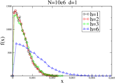
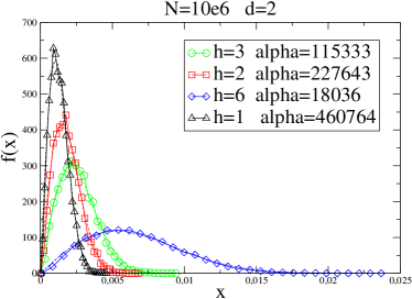
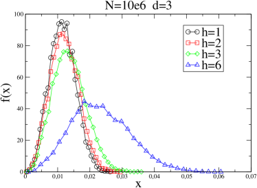
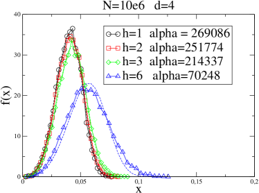
Figure 3.6: Radial distribution plot of exemplars obtained by clustering of Gaussian distributions of $N=10^{6}$ samples in ${\rm IR}^{d}$ in one single cluster exemplar, with hierarchical level $h$ ranging in 1,2,3,6, for diverse values of $d$: $d=1$ (upper left), $d=2$ (upper right), $d=3$ (bottom left) and $d=4$ (bottom right). Fitting functions are of the form $f(x)=Cx^{d/2-1}\exp(-\alpha x^{d/2})$.

Figure 3.6 shows the radial distribution of exemplars obtained with different hierarchy-depth $h$ and depending on the dimension $d$ of the dataset. The curve for $h=1$ corresponds to the AP case so the comparison with $h>1$ shows that the information loss due to the hierarchical approach is moderate to negligible in dimension $d\neq 2$ provided that the number of samples per cluster at each clustering level is “sufficient” (say, $M>30$ for the law of large numbers to hold). In dimension $d>2$, the distance of the center of mass to the origin is negligible with respect to its distance to the nearest exemplar; the distortion behaviour thus is given by the Weibull distribution which is stable by definition (with an increased sensitivity to small sample size $M$ as $d$ approaches 2). In dimension $d=1$, the distribution is dominated by the variance of the center of mass, yielding the gamma law which is also stable with respect to the hierarchical procedure. In dimension $d=2$ however, the Weibull and gamma laws do mix at the same scale; the overall effect is that the width of the distribution increases like $2^{h}$, as shown in Fig. 3.6 (top right).

We can also compute the corrections to this when $M$ is finite. We have the following property which is valid for (non necessarily spherical) distributions of sample points, with a finite variance $\sigma$.

Proposition 3.3.

For $d>2$, at level $h$, assume that

$$\alpha^{(h)}\stackrel{{\scriptstyle\mbox{\tiny def}}}{{=}}p_{sd}^{(h)}(0)\frac{\Omega_{d}}{d},$$ (3.6)

with $\Omega_{d}=2\pi^{d/2}/\Gamma(d/2)$ the $d$-dimensional solid angle, and

$$\sigma^{(h)}=\int d^{d}{\mbox{\bf r}}r^{2}p_{sd}^{(h)}({\mbox{\bf r}})$$

are both finite. Defining the shape factor of the distribution by

$$\omega^{(h)}\stackrel{{\scriptstyle\mbox{\tiny def}}}{{=}}\frac{\sigma^{(h)}{\alpha^{(h)}}^{2/d}}{\Gamma\bigl{(}1+\frac{2}{d}\bigr{)}},$$ (3.7)

the recurrence then reads,

$$\begin{cases}\displaystyle\sigma^{(h+1)}=\sigma^{(h)}\Bigl{(}1+\frac{\omega^{(h)}-\omega^{(h-1)}}{M^{1-2/d}}\Bigr{)}+o\bigl{(}M^{2/d-1}\bigr{)}.\\[5.69046pt] \displaystyle\omega^{(h+1)}=1+\frac{\omega^{(h)}}{M^{1-2/d}}+o\bigl{(}M^{2/d-1}\bigr{)}.\end{cases}$$ (3.8)

for $h>0$ and

$$\sigma^{(1)}=\frac{\sigma^{(0)}}{\omega^{(0)}}\Bigl{(}1+\frac{\omega^{(0)}}{M^{1-2/d}}\Bigr{)}+o\bigl{(}M^{2/d-1}\bigr{)},$$

Proof.

See appendix B. Note that the definition $\alpha^{(h)}$ is equivalent to the previous definition (3.4) if the distribution of sample points is regular (as well as for the variance $\sigma^{(h)}$ obviously).  

As a result, for $h=1$ we obtain

$$\sigma^{(2)}=\sigma^{(1)}\Bigl{(}1+\frac{1-\omega^{(0)}}{M^{1-2/d}}\Bigr{)}+o\bigl{(}M^{2/d-1}\bigr{)},$$

and thereby for $h>1$,

$$\sigma^{(h+1)} =\sigma^{(h)}+o\bigl{(}M^{2/d-1}\bigr{)},$$

$$=\frac{\sigma^{(0)}}{\omega^{(0)}}\Bigl{(}1+\frac{1}{M^{1-2/d}}\Bigr{)}+o\bigl{(}M^{2/d-1}\bigr{)}$$

This means that the mean error within the hierarchical procedure compared to the expected error scales like $N^{\frac{2}{hd}-\frac{1}{h}}$.

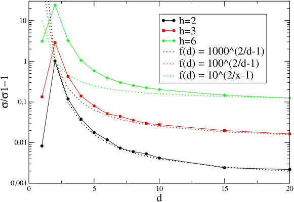
Figure 3.7: $\sigma_{ex}^{(h)}/\sigma_{ex}^{(1)}-1$ for $h=2,3,6$ as a function of the dimension, when finding exemplars of a single cluster of $10^{6}$ points (repeated $10^{4}$ times)

From definition (3.7) and (3.6), the relation between the shape factor $\omega$ and the variance $\sigma$ and the density $p_{0}$ near the center of mass reads,

$$\omega\stackrel{{\scriptstyle\mbox{\tiny def}}}{{=}}\frac{\bigl{(}\frac{d}{2}\bigr{)}^{1-2/d}\pi}{{\mbox{$\Gamma\bigl{(}\frac{2}{d}\bigr{)}$}}\bigl{(}\Gamma\bigl{(}\frac{d}{2}\bigr{)}\bigr{)}^{2/d}}\ p_{0}^{2/d}\sigma\operatorname*{\sim}_{d\to\infty}\frac{2}{d}p_{0}^{2/d}\sigma.$$

As its name indicates, it depends on the shape of the clusters. It relates the variance of the cluster to its density in the vicinity of the center of mass. In what follows it will be useful to keep in mind the following particular distributions in dimension $d$:

$$\omega=\begin{cases}\displaystyle\frac{d}{2}\frac{\pi}{{\mbox{$\Gamma\bigl{(}1+\frac{2}{d}\bigr{)}$}}},\qquad\text{Gaussian distribution}\\[11.38092pt] \displaystyle\frac{d}{d+2}\frac{1}{{\mbox{$\Gamma\bigl{(}1+\frac{2}{d}\bigr{)}$}}},\qquad\text{uniform $L2$-sphere distribution}\\[11.38092pt] \displaystyle\frac{\pi}{6}\frac{\bigl{(}\frac{d}{2}\bigr{)}^{2-2/d}}{{\mbox{$\Gamma\bigl{(}\frac{2}{d}\bigr{)}$}}\bigl{(}\Gamma\bigl{(}\frac{d}{2}\bigr{)}\bigr{)}^{2/d}},\qquad\text{uniform $L1$-sphere distribution},\end{cases}$$

while by our definition it is equal to unity for the Weibull distribution 3.5 yielded by the clustering procedure. In addition, for a superposition of clusters with identical forms and weights, represented by a distribution of the type (4.1), by simple inspection, the shape factor of the mixture is strictly greater than the single cluster shape factor, a soon as two cluster do not coincide exactly.

4 Renormalized affinity propagation (RAP)

The self-consistency of the Hi-AP procedure may be exploited to determine the underlying number of clusters present in a given data set. We follow here the guideline of the standard renormalization (or decimation) procedure which is used in statistical physics for analyzing scaling properties.

Figure 4.8:

basic scaling
Consider first a dataset, composed of $N$ items, occupying a region of total volume $V$, of a $d$-dimensional space, distributed according to a superposition of localized distributions,

$$f({\mbox{\bf r}})=\frac{1}{n^{*}}\sum_{c=1}^{n^{*}}\ {\sigma_{c}^{*}}^{-\frac{d}{2}}f_{0}\bigl{(}\frac{|{\mbox{\bf r}}-{\mbox{\bf r}}_{c}|}{\sqrt{\sigma_{c}^{*}}}\bigr{)},$$ (4.1)

where $n^{*}$ is the actual number of clusters, $f_{0}$ is a distribution normalized to one, ${\mbox{\bf r}}_{c}$ is the center of cluster $c$ and $\sigma_{c}^{*}$ the variance. Assume the data set is partitioned into $n=xV$ clusters, $x$ representing the density of these clusters, each cluster containing $N_{c}$ points and occupying an effective volume $V_{c}$. The energy (3.1) of the clustering reads for large $N$ and $n<<N$

$$E[{\bf c}] =\frac{1}{N}\sum_{c=1}^{xV}\Bigl{[}\sum_{i\in c}d^{2}(i,c)+\frac{N}{V}s\Bigr{]}$$

$$=\sigma(x)+xs,$$ (4.2)

where

$$\sigma(x) \stackrel{{\scriptstyle\mbox{\tiny def}}}{{=}}\frac{1}{N}\sum_{c=1}^{xV}\sum_{i\in c}d^{2}(i,c),$$

$$=\sum_{c=1}^{xV}\nu_{c}\sigma_{c},$$ (4.3)

is the distortion function, with $\nu_{c}=N_{c}/N$ is the fraction of data-point and $\sigma_{c}$ the corresponding variance of the AP-cluster $c$:

$$\sigma_{c}\stackrel{{\scriptstyle\mbox{\tiny def}}}{{=}}\int d^{d}{\mbox{\bf r}}f_{c}^{(AP)}({\mbox{\bf r}})({\mbox{\bf r}}-{\mbox{\bf r}}_{c})^{2}$$

by virtue of the law of large numbers. If $V_{c}$ represents the effective volume of such a cluster, we have

$$\sigma_{c}=V_{c}^{2/d}\tilde{\sigma}_{c},$$

where $\tilde{\sigma}_{c}$ is a dimensionless quantity. For $n\gg n^{*}$ we expect $V_{c}=V/n$ and $\tilde{\sigma}_{c}=\sigma$ (all AP-cluster have same spherical shape in this limit) so that

$$E[{\bf c}]\operatorname*{\sim}_{x\gg x^{*}}x^{-2/d}\sigma+xs.$$

For a given value of $s$, the optimal clustering is obtained for

$$x(s)=\Bigl{(}\frac{2\sigma}{ds}\Bigr{)}^{\frac{d}{2}}\qquad\qquad s\ll s^{*}.$$

self-consistency
Consider now a one step Hi-AP (see Figure 4.8) where the $N$-size data set is randomly partitioned into $M=1/\lambda$ subsets of $\lambda N$ points each and where the reduced penalty $s$ is fixed to some value such each clustering procedure yields $n$ exemplars in average. The resulting set of data points is then of size $n/\lambda$ and the question is how to adjust the value $s^{(\lambda)}$ for the clustering of this new data set, in order to recover the same result as the one which is obtained with a direct procedure with penalty $s$.

Figure 4.9:

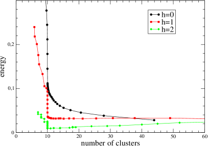
Figure 4.10: The distortion function for various values of $\eta$ for $d=5$ and $n^{*}=10,30$ (left panel).The energy (i.e.the distortion plus the penalties) as a function of the number of clusters obtained at each hierarchical level of a single Hi-AP procedure for $d=5$, $n^{*}=10$, $\eta=0.85$, $h=2$ and $\lambda N=300$ (right panel).

To answer to this question we make some hypothesis on the data set.

• (H1): the distribution of data points in the original set consists in a superposition of $n^{*}$ non-overlapping distributions, with common shape factor $\omega$ (3.7)

• (H2): there exists a value $s^{*}$ of $s$ for which AP yields the correct number of clusters $C$ when $N$ tends to infinity.

• (H3): $\sigma(x)$ which represents the mean square distance of the sample data to their exemplars in the thermodynamic limit, is assumed to be a smooth decreasing convex function of the density $x=n/V$ of exemplars (obtained by AP) with possibly a cusp at $x=x^{*}$ (see Figure 4.10).

The first hypothesis essentially amounts to assume that the clusters are “sufficiently” separated with respect to their size distribution. This can be characterized by the following parameter

$$\eta\stackrel{{\scriptstyle\mbox{\tiny def}}}{{=}}\frac{d_{min}}{2R_{max}},$$ (4.4)

where $d_{min}$ is the minimal mutual distance among clusters (between centers) and $R_{max}$ is the maximal value of cluster radius. We expect a good separability property for $\eta>1$. In practice this means the following. When $s$ is slowly increased, so that the number of cluster decreases unit by unit, the disappearing of a cluster corresponds either to some “true” cluster to be partitioned in on unit less, or either to two “true” clusters that are merged into a single cluster. The assumption (H2) amounts to say that the cost in distortion caused by merging two different true clusters is always greater than the cost corresponding to the fragmentation of one of the true clusters. As a result, starting from small values of $s$, and increasing it slowly, one is witnessing in the first part of the process a decrease in the fragmentation of the true clusters until some threshold value $s^{*}$ is reached. At that point this de-fragmentation process ends and is replaced by the merging process of the true clusters (see Figure 4.9). In the thermodynamic limit (which sustain all the present considerations), $s^{*}$ can be viewed as a critical value corresponding to a (presumably) second order phase transition, which separates a coalescent phase from a fragmentation phase. Note that when the second hypothesis (H2) is satisfied, this implied that (H1) is automatically satisfied by the dataset obtained after the first step of Hi-AP performed at $s^{*}$. Indeed, each partition of the initial set yields exactly one exemplar per true cluster in that case, and the rescaled distribution of these exemplars w.r.t their “true” center are universal after rescaling.

Figure 4.11: Sketch of the rescaling property. Comparison of the distortion function between two stages of Hi-AP (left panel). Corresponding result in terms of the number of clusters as a function of $s$.

The renormalization setting is depicted in Figure 4.8. The dataset is partitioned into $M=1/\lambda$ subsets. We manage that the size $\lambda N$ of each subset remain the same at each stage of the procedure. This means that $\lambda$ is set to $\lambda^{2}n$, if $n$ is the expected number of exemplars obtained at the corresponding stage. Under the two assumptions (H1) and (H2), the second step of Hi-AP, which corresponds to the clustering of $Nn/\lambda$ data points with a penalty set to $Nns(\lambda)/\lambda$ is expected to have the following property.

Proposition 4.1.

Let $n_{1}$ [resp. $n_{2}$] the number of clusters obtained after the first [resp. second] clustering step. If

$$s^{(\lambda)}=\frac{1}{\omega}\bigl{(}\frac{N\lambda}{n_{1}}\bigr{)}^{-\frac{2}{d}}\ s=\frac{\lambda^{2/d}}{\omega}\ s,\qquad\text{with}\qquad\frac{\lambda^{2/d}}{\omega}\ll 1,$$ (4.5)

then either cases occurs,

$$\begin{cases}s<s^{*}\qquad\text{then}\qquad n_{2}\geq n_{1}\geq n^{*}\\[5.69046pt] s=s^{*}\qquad\text{then}\qquad n_{2}=n_{1}=n^{*}.\\[5.69046pt] s>s^{*}\qquad\text{then}\qquad n_{2}=n_{1}\leq n^{*}\end{cases}$$

Proof.

In the thermodynamic limit the value $n_{1}$ for $n$, which minimizes the energy is obtained for $x_{1}=n_{1}/V$ as the minimum of (4.2):

$$s+\sigma^{\prime}(x_{1})=0.$$

At the second stage one has to minimize with respect to $x$,

$$E^{(\lambda)}[{\bf c}]=\frac{\lambda^{2/d}}{\omega}\Bigl{[}\frac{\omega}{\lambda^{2/d}}\sigma^{(\lambda)}(x,x_{1})+xs\Bigr{]},$$

where $\sigma^{(\lambda)}(x,y)$ denotes the distortion function of the second clustering stage when the first one yields a density $y$ of clusters. This amounts to find $x=x_{2}$ such that

$$s+\frac{\omega}{\lambda^{2/d}}\frac{\partial\sigma^{(\lambda)}}{\partial x}(x,x_{1})=0,$$ (4.6)

We need now to see how, depending on $x$,

$$\tilde{\sigma}_{x}^{(\lambda)}(y)\stackrel{{\scriptstyle\mbox{\tiny def}}}{{=}}\lambda^{-2/d}\sigma^{(\lambda)}(y,x)$$

compares with $\sigma(y)$. This is depicted on Figure 4.11.  

$\lambda N=300\qquad h=2\qquad n^{*}=10\qquad d=5$
$\eta=2.13$
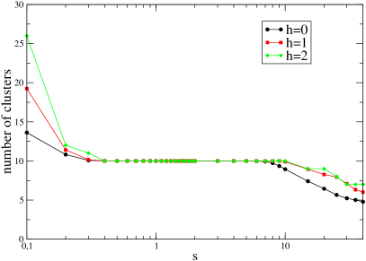
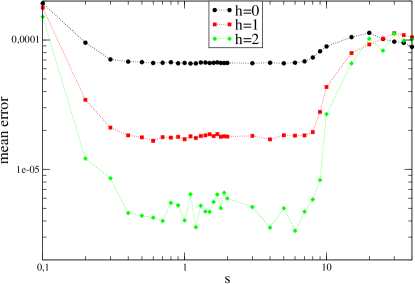
$\eta=0.85$
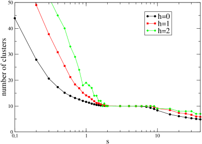
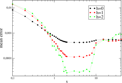
$\eta=0.54$

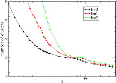
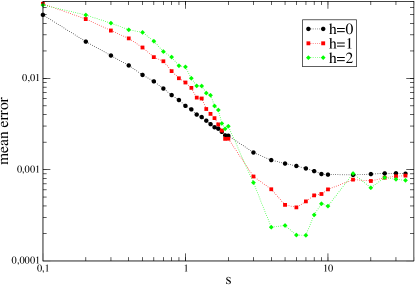
Figure 4.12: Number of cluster obtained in one single run with respect to the hierarchical level (left panel). Error distance of the exemplars from the true underlying centers obtained with respect to the hierarchical level (right panel). In all cases, $10$ underlying $L2$-sphere shaped clusters are present

$\eta=1.56\qquad n^{*}=10\qquad d=5$
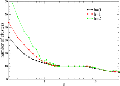
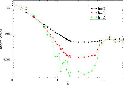
$\eta=0.85\qquad n^{*}=10\qquad d=5$
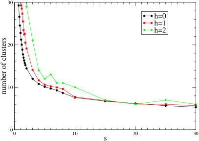
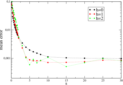
$\eta=0.4\qquad n^{*}=30\qquad d=5$
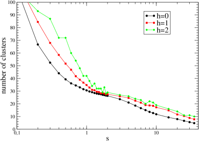
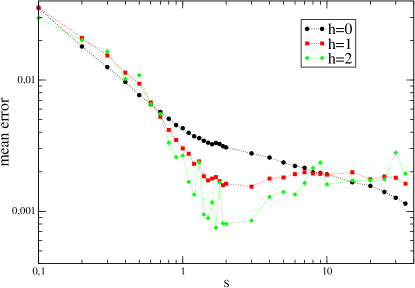
$\eta=0.36\qquad n^{*}=50\qquad d=5$

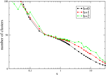
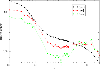
Figure 4.13: Number of clusters and mean-error as a function of $s$ for $L1$-sphere (first and second rows) and $L2$-sphere (third and fourth rows) shaped cluster.

$\eta=1.24\qquad n^{*}=10\qquad d=3$
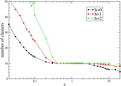
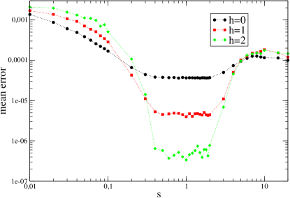
$\eta=1\qquad n^{*}=30\qquad d=5$
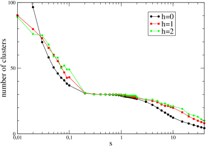
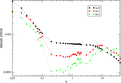
$\eta=0.66\qquad n^{*}=10\qquad d=10$
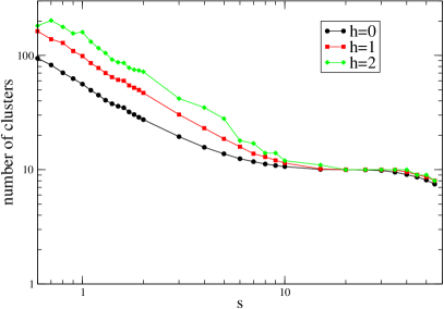
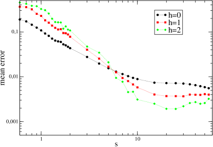
$\eta=1.33\qquad n^{*}=30\qquad d=20$

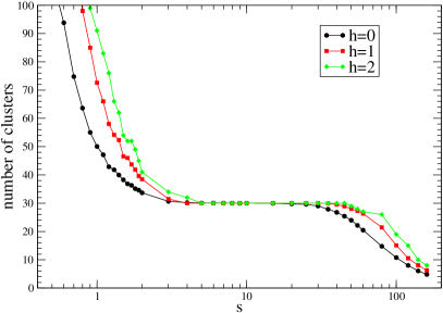
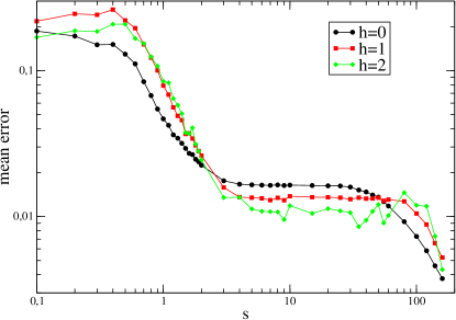
Figure 4.14: Number of clusters and mean-error as a function of $s$ for $L2$-sphere shaped in $d=3,5,10,20$ with $n^{*}=10,30,10$.

Assume first that $x_{1}=x^{*}$, which obtained if we set $s=s^{*}$ in the first clustering stage. This means that each cluster which is obtained at this stage is among the exact clusters with a reduced variance, resulting from the extreme value distribution properties (3.8) combined with definition (3.7) of the shape factor $\omega$:

$$\sigma_{c}^{(\lambda)}=\frac{1}{\omega}\Bigl{(}\frac{\lambda N}{n_{1}}\Bigr{)}^{-2/d}\sigma_{c}=\frac{\lambda^{2/d}}{\omega}\sigma_{c}.$$ (4.7)

Note at this point that

$$\frac{\omega}{\lambda^{2/d}}\gg 1,$$

is required to be in the conditions of getting a cluster shaped by the extreme value distribution. For $y>x^{*}$, the new distortion involves only the inner cluster distribution of exemplars which is simply rescaled by this $(x_{1}/\lambda)^{2/d}$ factor, so from (4.3) we conclude that

$$\tilde{\sigma}_{x^{*}}^{(\lambda)}(y)=\sigma(y),\qquad\text{for}\qquad y\geq x^{*}.$$

Instead, for $y<x^{*}$, the new distortion involves the merging of clusters, which inter distances, contrary to their inner distances, are not rescaled and are the same as in the original data set. This implies that

$$\frac{d\tilde{\sigma}_{x^{*}}^{(\lambda)}}{dy}(y)\leq\sigma^{\prime}(y),\qquad\text{for}\qquad y<x^{*}.$$

As a result the optimal number of clusters is unchanged, $y_{1}=x^{*}$.

For $x_{1}<x^{*}$, which is obtained when $s>s^{*}$, the new distribution of data points, formed of exemplars, is also governed by the extreme value distribution, and all cluster at this level are intrinsically true clusters, with a shape following the Weibull distribution. We are then necessary at the transition point at this stage: $y^{*}=x_{1}$. In addition, the cost of merging two clusters, i.e. $y$ slightly below $x_{1}$, is actually greater now after rescaling,

$$\frac{d\tilde{\sigma}_{x_{1}}^{(\lambda)}}{dy}(y)\leq\sigma^{\prime}(y),\qquad\text{for}\qquad y=(x_{1})_{-},$$

because mutual cluster distances appear comparatively larger. Instead, for $y$ slightly above $x_{1}$, the gain in distortion when $y$ increases is smaller, because it is due to the fragmentation of Weibull shaped cluster, as compared to the gain of separating clusters in the coalescence phase et former level,

$$\frac{d\tilde{\sigma}_{x_{1}}^{(\lambda)}}{dy}(y)\geq\sigma^{\prime}(y),\qquad\text{for}\qquad y=(x_{1})_{+}.$$

As a result, from the convexity property of $\sigma^{(\lambda)}(y)$, we then expect again that the solution of (4.6) remains unchanged $y_{1}=x_{1}$ in the second step with respect to the first one.

Finally, for $x_{1}>x^{*}$, the new distribution of data points is not shaped by the extreme value statistics when the number of fragmented clusters increases, because in that case the fragments are distributed in the entire volume of the fragmented cluster. In particular,

$$\tilde{\sigma}_{x_{1}}^{(\lambda)}(y)\simeq\frac{\omega}{\lambda^{2/d}}\sigma(y),\qquad\text{when}\qquad x_{1}>>x^{*}.$$

The rescaling effect vanishes progressively when we get away from the transition point, so we conclude that the optimal density of clusters $y_{1}$ is displaced toward larger values in this region.

We have tested this renormalized procedure, by generating artificial sets of datapoints in various situations, including different types of cluster shape. Some sample plots are displayed in Figure 4.12 and 4.13 to illustrate the preceding proposition 4.1. The self-similar point is clearly identified when plotting the number of clusters against the bare penalty, when $\eta$ is not to small. As expected from the scaling (4.5), the effect is less sensible when the dimension increases, but remains perfectly visible and exploitable at least up to $d=30$. The absence of information loss of the hierarchical procedure can be seen on the mean-error plots, in the region of $s$ around the critical value $s^{*}$. The results are stable, when we take into account at the first stage of the hierarchical procedure the influence of the shape of the clusters. This is done by fixing the value of the factor form $\omega$ to the correct value. In that case, at subsequent levels of the hierarchy the default value $\omega=1$ is the correct one to give consistent results. Nevertheless if the factor form is unknown and set to false default value, the results are spoiled at subsequent levels, and the underlying number of clusters turns out to be more difficult to identify, depending on the discrepancy of $\omega$ with respect to its default value. We see also that the identification of the transition point is still possible when the number of datapoints per cluster get smaller (down to $6$ in these tests).

5 Discussion and perspectives

The present analysis of the scaling properties of AP, within a divide-and-conquer setting gives us a simple way to identify a self-similar property of the special point $s^{*}$, for which the exact structure of the clusters is recovered. This property can be actually exploited, when the dimension is not too large and when the clusters are sufficiently far apart and sufficiently populated. The separability property is actually controlled by the parameter $\eta$ introduced in 4.4. For $\eta\geq 1$ the underlying cluster structure is recovered, and in the vicinity of $s^{*}$, the absence of information loss, deduced from the single cluster analysis is effectively observed. The search of the exact number of cluster could then be turned into a simple line-search algorithm combined with RAP. This deserves further exploration, in particular from the application point of view, on real data and for clusters of unknown shape. From the theoretical viewpoint, this renormalization approach to the self-tuning of algorithm parameter could be applied in other context, where self-similarity is a key property at large scale. First it is not yet clear how we could adapt RAP to the SCAP context. The principal component analysis and associated spectral clustering provide other examples, where the fixing of the number of selected components is usually not obtained by some self-consistent procedure and where a similar approach to the one presently proposed could be used.

Acknowledgments

This work was supported by the French National Research Agency (ANR) grant N° ANR-08-SYSC-017.

Appendix A Proof of Proposition 2.2

The influence between the center of mass and extreme value statistics distribution corresponds to corrections which vanish when $M$ tends to infinity (see Appendix B. Neglecting these corrections, enables us to use a spherical kernel instead of cylindrical kernel and to making no distinction between $ex$ and $\tilde{e}x$, to write the recurrence. Between level $h$ and $h+1$, one has:

$$f_{sd}^{(h+1)}(x)=\int_{0}^{\infty}K^{(h,M)}(x,y)f_{ex}^{(h,M)}(y)dy$$ (A.1)

with

$$\lim_{M\to\infty}M^{-1}K^{(h,M)}(\frac{x}{M},\frac{y}{M})=\frac{d}{\sigma^{(h)}}K(\frac{dx}{\sigma^{(h)}},\frac{dy}{\sigma^{(h)}})$$ (A.2)

where $K(x,y)$ is the d-dimensional radial diffusion kernel,

$$K(x,y)\stackrel{{\scriptstyle\mbox{\tiny def}}}{{=}}\frac{1}{2}x^{\frac{d-2}{4}}y^{\frac{2-d}{4}}I_{\frac{d-2}{2}}\bigl{(}\sqrt{xy}\bigr{)}e^{-\frac{x+y}{2}}.$$

with $I_{\frac{d}{2}-1}$ the modified Bessel function of index ${d/2-1}$. The selection mechanism of the exemplar yields at level $h$,

$$F_{ex}^{(h,M)}(x)=\bigl{(}F_{sd}^{(h)}(x)\bigr{)}^{M},$$

and with a by part integration, (A.1) rewrites as:

$$f_{sd}^{(h+1)}(x) = K^{(h,M)}(x,0)+$$

$$\int_{0}^{\infty}\bigl{(}F_{sd}^{(h)}(y)\bigr{)}^{M}\ \frac{\partial K^{(h,M)}}{\partial y}(x,y)dy,$$

with

$$\lim_{M\to\infty}M^{-1} K^{(h,M)}(\frac{x}{M},0)=$$

$$\frac{d}{2\Gamma(\frac{d}{2})\sigma^{(h)}}\bigl{(}\frac{dx}{2\sigma^{(h)}}\bigr{)}^{\frac{d}{2}-1}\exp\bigl{(}-\frac{dx}{2\sigma^{(h)}}\bigr{)}.$$

At this point the recursive hierarchical clustering is described as a closed form equation. Proposition 3.2 is then based on (A.2) and on the following scaling behaviors,

$$\lim_{M\to\infty}F_{ex}^{(h,M)}\bigl{(}\frac{x}{M^{\frac{2}{d}}}\bigr{)}=\exp\bigl{(}-\alpha^{(h)}x^{\frac{d}{2}}\bigr{)},$$

so that

$$\lim_{M\to\infty}F_{sd}^{(h+1)}(\frac{x}{M^{\gamma}}) =\lim_{M\to\infty}M^{1-\gamma}\int_{0}^{\infty}dy$$

$$\int_{\frac{x}{\sigma^{(h)}}}^{\infty}du f_{ex}^{(h,M)}(\frac{y}{M^{\frac{2}{d}}})K(M^{1-\gamma}u,\frac{M^{1-\frac{d}{2}}y}{\sigma^{(h)}}).$$

Basic asymptotic properties of $I_{d/2-1}$ yield with a proper choice of $\gamma$, the non degenerate limits of proposition 3.2. In the particular case $d=2$, taking $\gamma=1$, it comes:

$$\lim_{M\to\infty}F_{sd}^{(h+1)}(\frac{x}{M})=\int_{0}^{\infty}dy\int_{\frac{x}{\sigma^{(h)}}}^{\infty}duf_{ex}^{(h)}(\sigma^{(h)}y)K(u,y)\\$$

$$\quad=-\int_{0}^{\infty}dy\int_{\frac{x}{\sigma^{(h)}}}^{\infty}du\frac{de^{-\alpha^{(h)}\sigma^{(h)}x}}{dy}I_{0}(2\sqrt{uy})e^{-(u+y)}\\$$

$$=\exp\bigl{(}-\frac{\alpha^{(h)}}{1+\alpha^{(h)}\sigma^{(h)}}x\bigr{)},\qquad\qquad\qquad\qquad$$

with help of the identity

$$\int_{0}^{\infty}dxx^{\nu}e^{-\alpha x}I_{2\nu}(2\beta\sqrt{x})=\frac{1}{\alpha}\bigl{(}\frac{\beta}{\alpha}\bigr{)}^{2\nu}e^{\frac{\beta}{\alpha}}.$$

Again in the particular case $d=2$, by virtue of the exponential law one further has $\alpha^{(h)}=1/\sigma^{(h)}$, finally yielding:

$$\beta^{(h+1)}=\frac{1}{2}\beta^{(h)}.$$ (A.3)

Appendix B Finite size corrections

We consider a given hierarchical level $h$, r denotes sample points, ${\mbox{\bf r}}_{cm}$ their corresponding center of mass, and r${}_{{\mbox{\bf c}}}$ the exemplar, which in turn becomes a sample point at level $h+1$. We have

$$p_{sd}^{(h+1)}({\mbox{\bf r}})d^{d}{\mbox{\bf r}} =P({\mbox{\bf r${}_{{\mbox{\bf c}}}$}}\in d^{d}{\mbox{\bf r}})$$

$$=d^{d}{\mbox{\bf r}}\int d^{d}{\mbox{${\mbox{\bf r}}_{cm}$}}p_{sd,cm}^{(h)}({\mbox{\bf r}},{\mbox{${\mbox{\bf r}}_{cm}$}})P(|{\mbox{${\mbox{\bf r}}_{sd}$}}-{\mbox{${\mbox{\bf r}}_{cm}$}}|\geq|{\mbox{\bf r}}-{\mbox{${\mbox{\bf r}}_{cm}$}}|\big{|}{\mbox{${\mbox{\bf r}}_{cm}$}})^{M-1}.$$

We analyse this equation with the help of a generating function:

$$\phi_{\centerdot}(\Lambda)=\int d^{d}{\mbox{\bf r}}p_{\centerdot}({\mbox{\bf r}})e^{-\Lambda{\mbox{\bf r}}}.$$

where $\centerdot$ may be indifferently $sd$, $c$ or $cm$ and $\Lambda{\mbox{\bf r}}$ is the ordinary scalar product between two $d$-dimensional vectors. Let $\lambda=|\Lambda|$, by rotational invariance, $p_{\centerdot}$ depends only on $r$ and $\phi_{\centerdot}$ depends solely on $\lambda$, so we have

$$g_{\centerdot}(\lambda)\stackrel{{\scriptstyle\mbox{\tiny def}}}{{=}}\log(\phi_{\centerdot}(\Lambda))=\log\Bigl{(}2\pi^{d/2}\int_{0}^{\infty}drr^{d-1}p_{\centerdot}(r)\bigl{(}\frac{\lambda r}{2}\bigr{)}^{1-d/2}I_{d/2-1}(\lambda r)\Bigr{)}.$$

The joint distribution between ${\mbox{\bf r}}_{sd}$ and ${\mbox{\bf r}}_{cm}$ takes the following form

$$p_{sd,cm}({\mbox{\bf r}},{\mbox{${\mbox{\bf r}}_{cm}$}})=p_{sd}(r)p_{cm|sd}(|{\mbox{${\mbox{\bf r}}_{cm}$}}-\frac{{\mbox{\bf r}}}{M}|)$$

where by definition $p_{cm|sd}$ is the conditional density of ${\mbox{\bf r}}_{cm}$ to ${\mbox{\bf r}}_{sd}$, with

$$g_{cm|sd}(\lambda)=(M-1)g_{sd}\bigl{(}\frac{\lambda}{M}\bigr{)},$$ (B.1)

while

$$g_{cm}(\lambda)=Mg_{sd}\bigl{(}\frac{\lambda}{M}\bigr{)},$$ (B.2)

where $g_{sd}$ is assumed to have a non zero radius Taylor expansion of the form

$$g_{sd}(\lambda)=\frac{\sigma^{(h)}}{2d}\lambda^{2}+\sum_{n=2}^{\infty}\frac{g^{(2n)}(0)}{2n!}\lambda^{2n},$$ (B.3)

since by rotational symmetry all odd powers of $\lambda$ vanish and where $\sigma^{(h)}$ represents the variance at level $h$ of the sample data distribution. In addition the conditional probability density of ${\mbox{\bf r}}_{sd}$ to ${\mbox{\bf r}}_{cm}$ reads

$$p_{sd|cm}({\mbox{\bf r}},{\mbox{${\mbox{\bf r}}_{cm}$}})=\frac{p_{sd}(r)}{p_{cm}(r_{cm})}p_{cm|sd}(|{\mbox{${\mbox{\bf r}}_{cm}$}}-\frac{{\mbox{\bf r}}}{M}|)\stackrel{{\scriptstyle\mbox{\tiny def}}}{{=}}p_{sd|cm}(u,\theta,r_{cm})$$

where ${\bf u}={\mbox{\bf r}}-{\mbox{${\mbox{\bf r}}_{cm}$}}$ and $\theta$ is the angle between ${\bf u}$ and ${\mbox{\bf r}}_{cm}$. Let

$$f(u,r_{cm})\stackrel{{\scriptstyle\mbox{\tiny def}}}{{=}}P(|{\mbox{${\mbox{\bf r}}_{sd}$}}-{\mbox{${\mbox{\bf r}}_{cm}$}}|\geq u\big{|}{\mbox{${\mbox{\bf r}}_{cm}$}}).$$

We have

$$f(u,r_{cm})=1-\Omega_{d-1}\int_{0}^{u}dxx^{d-1}\int_{0}^{\pi}d\theta\sin\theta^{d-2}p_{sd|cm}(x,\theta,r_{cm}).$$

with

$$\Omega_{d}=\frac{2\pi^{d/2}}{\Gamma\bigl{(}\frac{d}{2}\bigr{)}},$$

the $d$-dimensional solid angle. Let

$$h(u,r_{cm})\stackrel{{\scriptstyle\mbox{\tiny def}}}{{=}}\log(f(u,r_{cm})).$$

We have

$$p_{sd}^{(h+1)}(r)=p_{sd}^{(h)}(r)\int d^{d}{\mbox{${\mbox{\bf r}}_{cm}$}}p_{cm|sd}(|{\mbox{${\mbox{\bf r}}_{cm}$}}-\frac{{\mbox{\bf r}}}{M}|)\exp\bigl{(}(M-1)h(|{\bf r}-{\mbox{${\mbox{\bf r}}_{cm}$}}|,r_{cm})\bigr{)}.$$

From the expansion (B.3) we see that corrections in $g_{cm}$ and $g_{cm|sd}$ to the Gaussian distribution are of order $1/M^{3}$, $\sigma_{cm}=\sigma/M$ as expected from the central limit theorem and $\sigma_{cm|sd}=(M-1)\sigma/M^{2}$. Letting ${\bf}y={\bf r}_{cm}-{\bf r}$ we have

$$p_{sd}^{(h+1)}(r)=p_{sd}^{(h)}(0)\Bigl{(}\frac{dM}{2\pi\sigma^{(h)}}\Bigr{)}^{d/2}\int d^{d}{\bf y}\ \exp\Bigl{(}-M\psi^{(M)}({\bf r},{\bf y})\Bigr{)},$$

with

$$\psi^{(M)}({\bf r},{\bf y}) \stackrel{{\scriptstyle\mbox{\tiny def}}}{{=}}-\frac{d}{2}\log\frac{M}{M-1}-\frac{dr^{2}}{2\sigma^{(h)}}+\log\frac{p_{sd}^{(h)}(r)}{p_{sd}^{(h)}(0)}$$

$$+\frac{dM}{2(M-1)\sigma^{(h)}}|{\bf y+r}|^{2}+(M-1)h\bigl{(}y,|{\bf y+r}|\bigr{)}.$$

As observed previously $p_{sd}^{(h+1)}(r/M^{1/d})$ converges to a Weibull distribution when $M$ goes to infinity, and the corrections to this are obtained with help of the following approximation:

$$\psi^{(M)}(\frac{\bf r}{M^{1/d}},{\bf y})=\frac{d}{2\sigma^{(h)}}|{\bf y}+\frac{\bf r}{M^{1/d}}|^{2}+\alpha^{(h)}y^{d}+O\bigl{(}\frac{1}{M}\bigr{)},\\$$

with

$$\alpha^{(h)}=p_{sd}^{(h)}(0)\frac{\Omega_{d}}{d}.$$

As a result, computing the normalization constant $p_{sd}^{(h+1)}(0)$ and the corresponding variance $\sigma^{(h+1)}$, yields the following recurrence relations:

$$\begin{cases}\displaystyle\alpha^{(h+1)}=\alpha^{(h)}\ +\ O\Bigl{(}\frac{1}{M}\Bigr{)}.\\[8.5359pt] \displaystyle\sigma^{(h+1)}=\Gamma\bigl{(}1+\frac{2}{d}\bigr{)}{\alpha^{(h)}}^{-2/d}\Bigl{(}1+\frac{\sigma^{(h)}\alpha^{2/d}}{{\mbox{$\Gamma\bigl{(}1+\frac{2}{d}\bigr{)}$}}}\frac{1}{M^{1-2/d}}\Bigr{)}+o\bigl{(}M^{2/d-1}\bigr{)}.\end{cases}$$

Letting

$$\omega^{(h)}\stackrel{{\scriptstyle\mbox{\tiny def}}}{{=}}\frac{\sigma^{(h)}{\alpha^{(h)}}^{2/d}}{\Gamma\bigl{(}1+\frac{2}{d}\bigr{)}},$$

we get

$$\omega^{(h+1)}=1+\frac{\omega^{(h)}}{M^{1-2/d}}+o\bigl{(}M^{2/d-1}\bigr{)}.$$

Consequently, for $h=0$, we have

$$\sigma^{(1)}=\frac{\sigma^{(0)}}{\omega^{(0)}}\Bigl{(}1+\frac{\omega^{(0)}}{M^{1-2/d}}\Bigr{)}+o\bigl{(}M^{2/d-1}\bigr{)},$$

while for $h>1$ we get

$$\sigma^{(h+1)}=\sigma^{(h)}\Bigl{(}1+\frac{\omega^{(h)}-\omega^{(h-1)}}{M^{1-2/d}}\Bigr{)}+o\bigl{(}M^{2/d-1}\bigr{)}.$$

For $h=1$ this reads

$$\sigma^{(2)}=\sigma^{(1)}\Bigl{(}1+\frac{1-\omega^{(0)}}{M^{1-2/d}}\Bigr{)}+o\bigl{(}M^{2/d-1}\bigr{)},$$

and thereby

$$\sigma^{(h+1)}=\sigma^{(h)}+o\bigl{(}M^{2/d-1}\bigr{)},\qquad\text{for}\ h>1.$$

References

- [1] J. Pearl. Probabilistic Reasoning in Intelligent Systems: Network of Plausible Inference. Morgan Kaufmann, 1988.
- [2] F. R. Kschischang, B. J. Frey, and H. A. Loeliger. Factor graphs and the sum-product algorithm. IEEE Transactions on Information Theory, 47:498–519, 2001.
- [3] J. S. Yedidia, W. T. Freeman, and Y. Weiss. Generalized belief propagation. Advances in Neural Information Processing Systems, pages 689–695, 2001.
- [4] M. Mézard and R. Zecchina. The random K-satisfiability problem: from an analytic solution to an efficient algorithm. Phys.Rev.E 66, page 56126, 2002.
- [5] B. Frey and D. Dueck. Clustering by passing messages between data points. Science, 315:972–976, 2007.
- [6] M. Leone, Sumedha, and M. Weigt. Clustering by soft-constraint affinity propagation: Applications to gene-expression data. Bioinformatics, 23:2708, 2007.
- [7] M. Leone, Sumedha, and M. Weigt. Unsupervised and semi-supervised clustering by message passing: Soft-constraint affinity propagation. Eur. Phys. J. B, pages 125–135, 2008.
- [8] A.P. Dempster, Laird N.M., and D.B. Rubin. Maximum likelihood for incomplete data via the em algorithm. J. Royal Stat. Soc. B, 39(1):1–38, 1977.
- [9] C. Fraley and A. Raftery. How many clusters?which clustering method? answer via model-based clustering. The Computer Journal, 41(8), 1998.
- [10] S. Still and W. Bialek. How many clusters?:an information-theoretic perspective. Neural Computation, 16:2483–2506, 2004.
- [11] S. Dudoit and J. Fridlyand. A prediction-based resampling method for estimating the number of clusters in a dataset. Genome Biology, 2(7):0036.1–0036.21, 2002.
- [12] K. Wang, J. Zhang, D. Li, X. Zhang, and T. Guo. Adaptive affinity propagation clustering. Acta Automatica Sinica, 33(12):1242–1246, 2007.
- [13] X. Zhang, C. Furtlehner, and M. Sebag. Data streaming with affinity propagation. In ECML/PKDD, pages 628–643, 2008.
- [14] X. Zhang, J. Furtlehner, C. Perez, C. Germain-Renaud, and M. Sebag. Toward autonomic grids: Analyzing the job flow with affinity streaming. In KDD, pages 628–643, 2009.
- [15] Y. Kabashima. Propagating beliefs in spin-glass models. J. Phys. Soc. Jpn., 72:1645–1649, 2003.
- [16] H. A. Bethe. Statistical theory of superlattices. Proc. Roy. Soc. London A, 150(871):552–575, 1935.
- [17] S. Guha, A. Meyerson, N. Mishra, R. Motwani, and L. O’Callaghan. Clustering data streams: Theory and practice. In TKDE, volume 15, pages 515–528, 2003.
- [18] L. de Haan and A. Ferreira. Extreme Value Theory. Operations Research and Financial Engineering. Springer, 2006.