Comparison of the thin flux tube approximation with 3D MHD simulations

Abstract

Context. The structure and dynamics of small vertical photospheric magnetic flux concentrations has been often treated in the framework of an approximation based upon a low-order truncation of the Taylor expansions of all quantities in the horizontal direction, together with the assumption of instantaneous total pressure balance at the boundary to the non-magnetic external medium. Formally, such an approximation is justified if the diameter of the structure (a flux tube or a flux sheet) is small compared to all other relevant length scales (scale height, radius of curvature, wavelength, etc.). The advent of realistic 3D radiative MHD simulations opens the possibility of checking the consistency of the approximation with the properties of the flux concentrations that form in the course of a simulation.

Aims. We carry out a comparative analysis between the thin flux tube/sheet models and flux concentrations formed in a 3D radiation-MHD simulation.

Methods. We compare the distribution of the vertical and horizontal components of the magnetic field in a 3D MHD simulation with the field distribution in the case of the thin flux tube/sheet approximation. We also consider the total (gas plus magnetic) pressure in the MHD simulation box.

Results. Flux concentrations with super-equipartition fields are reasonably well reproduced by the second-order thin flux tube/sheet approximation. The differences between approximation and simulation are due to the asymmetry and the dynamics of the simulated structures.

1 Introduction

Much of the solar photospheric magnetic flux exists in the form of discrete concentrations in intergranular lanes having a field strength of 1-2 kG (Stenflo, 1973; Wiehr, 1978; Rüedi et al., 1992; Rabin, 1992; Martínez Pillet et al., 1997), for reviews see Solanki (1993); Solanki et al. (2006).

Theoretical models of these flux concentrations have widely used the concept of the flux tube: a bundle of field lines with circular cross-section separated from the non-magnetic environment by a tangential discontinuity (see e.g. Schüssler, 1992). Such a structure can be described, under certain conditions, by the so called ”thin flux tube approximation ”. In its simplest form, the axial component of the magnetic field is assumed to be constant across the tube’s cross-section, while the radial component is a linear function of the radial coordinate (Defouw, 1976; Roberts & Webb, 1978, 1979). The thin flux tube approximation can be formally justified if the diameter of the flux tube is sufficiently small compared to variations of the relevant physical quantities (such as pressure, density,$...$etc.) along the tube’s cross-section (Spruit, 1981; Schüssler, 1992).

The equations describing a thin flux tube can be obtained by writing all physical quantities (magnetic field, temperature, pressure,$...$etc) in terms of a Taylor expansion in the radial distance from the axis, and inserting them in the MHD equations. By collecting terms of similar order one obtains a hierarchy of equations (Ferriz-Mas & Schüssler, 1989). Truncating this hierarchy after the $1^{st}$ order allows the $0^{th}$-order approximation introduced above to be obtained.

Extensions of the thin flux tube approximation to higher orders have been given in the literature. By retaining second-order terms Pneuman et al. (1986) have included in their modelling the effects of field line curvature, internal structures, twist, and the merging of flux tubes with their neighbours. A derivation of linear wave modes of a flux tube up to second order has been carried out by Ferriz-Mas et al. (1989).

There is a large body of work in the literature based upon the thin flux tube approximation. This includes theoretical work (structure of flux concentrations, equilibrium, oscillations/wave, stability,…etc.) and interpretation of observations (for reviews, see Solanki, 1993; Solanki et al., 2006). Various aspects of the thin tube approximation have been compared to observational data (e.g. Zayer et al., 1989; Bruls & Solanki, 1995; Solanki et al., 1996), but its validity has not been tested on the basis of the most advanced numerical simulations.

In the last two decades, the possibilities to self consistently model magneto-convection at the solar photosphere using the full set of MHD equations including radiative and convective energy transport (e.g. Nordlund, 1983; Stein & Nordlund, 1998; Bercik, 2002; Stein & Nordlund, 2003; Vögler & Schüssler, 2003; Vögler et al., 2005) have greatly improved. The structure of flux concentrations in such MHD simulations appears rather complex, owing to their interaction with convection and energy exchange with the neighbouring plasma.

We aim to evaluate to which extent the magnetic structures forming in 3D MHD simulations can be described using the thin flux tube/sheet approximation.

2 A series expansion of the thin flux tube/sheet equations

We consider a magnetic flux tube to be a bundle of magnetic field lines with a circular cross section, which is separated from its non-magnetic surroundings by a tangential discontinuity with a surface current. For an axisymmetric vertical flux tube, we adopt cylindrical coordinates ($r$,$\theta$,$z$), with the $z$-axis pointing in the vertical direction. Physical quantities are regular at the axis ($r=0$), so that they can be described in terms of a Taylor expansion in the radial coordinate (Roberts & Webb, 1978; Spruit, 1981; Pneuman et al., 1986; Ferriz-Mas et al., 1989; Ferriz-Mas & Schüssler, 1989)

The properties of the axisymmetric MHD equations (Ferriz-Mas & Schüssler, 1989) imply that only even orders are non-zero in the above-mensioned expansions for scalar quantities (such as temperature or density) and for $z$-components of vectors, whereas for the radial and $\theta$-components of vectors only the odd orders remain.

The three components of the magnetic field vector, the temperature and the pressure can be written in a non-dimensional way:

$$b_{z}=h_{0}+h_{2}x^{2}+h_{4}x^{4}+...,$$ (1)

$$b_{r}=f_{1}x+f_{3}x^{3}+f_{5}x^{5}+...,$$ (2)

$$b_{\theta}=s_{1}x+s_{3}x^{3}+s_{5}x^{5}+...$$ (3)

$$p=p_{0}+p_{2}x^{2}+p_{4}x^{4}+...$$ (4)

$$\sigma=\sigma_{0}+\sigma_{2}x^{2}+\sigma_{4}x^{4}+...,$$ (5)

with $p=P/P^{*}$, $\sigma=T/T^{*}$, $b=B/B^{*}$, $x=r/H^{*}$, $y=z/H^{*}$, $H^{*}=kT^{*}/(m_{p}g)$ and $\alpha=4\pi P^{*}/B^{*2}$. Where $B_{r}$, $B_{\theta}$, $B_{z}$, represent the three components of the magnetic field vector. $P$ and $T$ are the gas pressure and temperature, respectively. The quantities with an asterisk are defined at the tube’s axis ($x=r=0$) and at a reference height ($z=y=0$). $k$ is Boltzmann’s constant, $m_{p}$ the mean particle mass, $g$ the gravitational acceleration, and $H$ the scale height.

2.1 $B_{z}$ and $B_{r}$ under the thin flux tube approximation

Following, e.g., Pneuman et al. (1986), in a static atmosphere, we insert the expansions (1 to 5) in the three components of the momentum equation and the solenoidality relation, and collect terms of equal power in $x$ into equations of corresponding order. Considering equations including terms up to the third order, and assuming that the flux tubes studied here have negligible twist, we obtain the following relations (Pneuman et al., 1986):

$$h_{2}=-\frac{1}{4}h^{\prime\prime}_{0}-\frac{\alpha p_{2}}{h_{0}},$$ (6)

$$f_{1}=-\frac{1}{2}h^{\prime}_{0},$$ (7)

and

$$f_{3}=-\frac{1}{4}h^{\prime}_{2},$$ (8)

where the prime indicates a derivative with respect to $y$

We can then deduce $B_{z}$ up to the second order, and $B_{r}$ up to the third order.

In order to close the above system it is necessary to consider relations expressing magnetic flux conservation through the tube’s cross-section and total pressure balance at the boundary of the flux tube at any height (Ferriz-Mas & Schüssler, 1989; Ferriz-Mas et al., 1989). In addition to these relations, Ferriz-Mas et al. (1989) have considered an energy equation, whereas Pneuman et al. (1986) have chosen to prescribe two quantities, such as $\sigma_{0}$ and $\sigma_{2}$, which allows more flexibility in defining the atmosphere. In order to construct a thin flux tube which we will compare with flux concentrations in MHD simulations, we take $h_{0}$ and $p_{2}$ from the MHD simulations. Then $B_{z}$ and $B_{r}$ are determined from equations (6) to (8). The cross section of the flux tube is determined through the magnetic flux conservation relation:

$$\int_{0}^{x_{0}}(h_{0}+h_{2}x^{2})dx=\mathrm{Flux\leavevmode\nobreak\ at\leavevmode\nobreak\ base\leavevmode\nobreak\ of\leavevmode\nobreak\ tube}=\mathrm{constant},$$ (9)

where $x_{0}$ is the tube’s radius at a given height. The total pressure balance can be expressed as:

$$(\beta p_{i}+b_{i}^{2})|_{x=x_{0}}=(8\pi P_{e}+B_{e}^{2})/B^{*2}|_{x=x_{0}},$$ (10)

where $\beta=8\pi P^{*}/B^{*2}$, the suffixes $i$ and $e$ indicate internal and external quantities respectively and capital letters indicate dimensional quantities.

Under the $0^{th}$-order approximation Eq. (10) reduces to:

$$(\beta p_{0}+h_{0}^{2})|_{x=x_{0}}=(8\pi P_{e}+B_{e}^{2})/B^{*2}|_{x=x_{0}},$$ (11)

This relation does not depend on the radius of the flux tube. Thus the total pressure at a given height under the $0^{th}$-order approximation is constant across the tube’s cross-section.

Under the $2^{nd}$-order approximation we get:

$$(\beta p_{0}+h_{0}^{2})+x^{2}(\beta p_{2}+f_{1}^{2}+2h_{0}h_{2})|_{x=x_{0}}=(8\pi P_{e}+B_{e}^{2})/B^{*2}|_{x=x_{0}},$$ (12)

In this case the total pressure varies inside the flux tube, but has to match the external total pressure at the tube’s boundary.

2.2 $B_{z}$ and $B_{x}$ under the thin flux sheet approximation

A flux sheet is an elongated structure with a small width (which we refer to as $"W"$) compared to its length ($"L"$) along the solar surface, i.e. $W<<L$ at the solar surface. A similar approach as described in the previous section can be used to describe a thin flux sheet. In this case the magnetic field component parallel to $L$ is constant, and thus plays no direct role in the hydrostatic equilibrium. We can then adopt a Cartesian $2D$ geometry in the $x-z$ plane, where $z$ is the vertical coordinate and $x$ is the horizontal coordinate perpendicular to the vector $L$.

In a similar way to Sect. 2.1, we can determine $h_{2}$, $f_{1}$ and $f_{3}$ as functions of $h_{0}$ and $p_{2}$.

$$h_{2}=-\frac{1}{2}h^{\prime\prime}_{0}-\frac{\alpha p_{2}}{h_{0}}$$ (13)

$$f_{1}=-h^{\prime}_{0}$$ (14)

and

$$f_{3}=-\frac{1}{3}h^{\prime}_{2}$$ (15)

Note the similarity between these equations and the ones describing the thin flux tube. The main difference (apart of the geometry) is the numerical values of the constant coefficients which affects, for instance, the expansion rate of the flux tube/sheet with height.

3 The radiative MHD simulations

Three dimensional radiation-MHD simulations of the solar photosphere have been described by (Nordlund, 1983; Nordlund & Stein, 1990; Stein & Nordlund, 1998; Bercik, 2002; Stein & Nordlund, 2003; Vögler & Schüssler, 2003; Vögler et al., 2005).

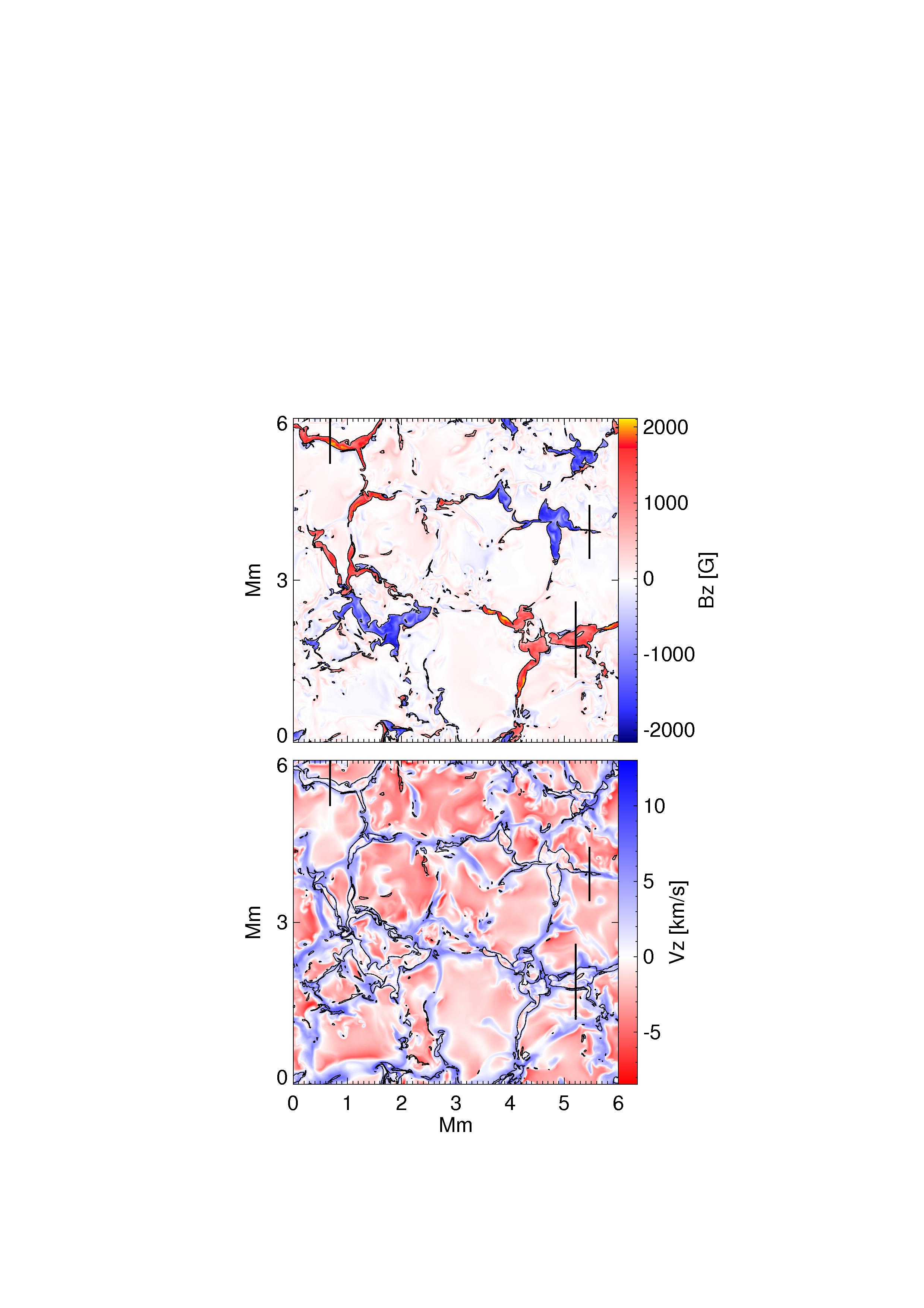
Figure 1: Upper panel: vertical component of the magnetic field ($B_{z}$) at a fixed geometrical height near the averaged visible solar surface ($\tau_{5000}=1$). Lower panel: vertical component of the velocity ($V_{z}$) at $\tau_{5000}=1$. Downflows are represented in red and upflows in blue. The black contours outline regions where $|B_{z}|>500$ G. The black vertical lines indicate locations where we carry out a detailed analysis of magnetic elements in Section 5.

The simulation run used here has been obtained with the fully compressible MURaM code (Vögler, 2003; Vögler et al., 2005). It takes into account non-local and non-gray radiative energy transport, and includes the effects of partial ionization. The simulation box has a horizontal extension of $6\times 6$ $\mathrm{Mm}^{2}$ and is $1.4$ Mm deep. The grid cell size is 5 km in the horizontal direction and 7 km in the vertical. The simulation run starts from a plane-parallel atmosphere which extends from $-0.8$ Mm below to $0.6$ Mm above a reference $0$, which is roughly situated $-100$ km below the average continuum optical depth unity ($\tau_{5000}=1$, which corresponds to the solar surface at $5000$ Å). After convection has fully developed, a mixed-polarity magnetic field configuration with zero net vertical flux is introduced. This is done such that the simulation domain is divided into four parts with vertical field of alternate polarities in a chessboard pattern. We choose a representative snapshot for our analysis (see Fig. 1). The mean unsigned field strength at optical depth unity is $200$ G for this snapshot.

4 Analysis of the total pressure in the whole simulation domain

Figure 2 shows horizontally averaged gas and total pressures as a function of height. The solid line represents the gas pressure averaged over regions with field strength smaller than 50 G. The dash-dotted line indicates the gas pressure averaged over magnetic regions. The threshold in $|B_{z}|$ defining magnetic regions varies linearly from $500$ G at the bottom of the simulation box to $300$ G at the top. The dashed line represents the total pressure ($P_{tot}$=$P+B^{2}/(8\pi)$) averaged over magnetic regions. The plasma $\beta=8\pi P/B^{2}$ for magnetic regions is indicated by square symbols.

The difference between the gas pressures inside and outside magnetic regions becomes smaller with depth. This is due to the large values of the plasma $\beta$ in the deep layers (e.g. below $-400$ km) which indicate that the pressure balance between magnetic features and their surroundings is mainly ensured by gas pressure. Above $300$ km, the total pressure in magnetic features shows an excess compared to gas pressure in nearly field-free areas. This excess increases with height and is due to the effect of curvature forces. This implies that the $0^{th}$-order thin flux tube/sheet approximation is not sufficient to describe the flux concentrations in the upper part of the simulation box. The gas pressure in nearly field-free regions is higher than the total pressure in the flux concentrations in the height-range situated between $50$ and $300$ km. This slight pressure excess mainly results from the fact that the gas pressure at equal geometrical height is, on average, higher in the granular upflows than in the intergranular downflow lanes, where the magnetic flux concentrations reside. In addition, a pressure deficit in the flux concentrations relative to their local environment could arise as the result of the outward curvature force of the expanding tubes between $0$ and $300$ km height. Above $300$ km, the sign of the curvature force is reversed as a result of the wineglass shape of the flux tubes caused by the presence of neighboring tubes (reflected in our simulation by the vertical-field upper boundary condition). In any case, the deviation from total pressure balance is very small below $300$ km height.

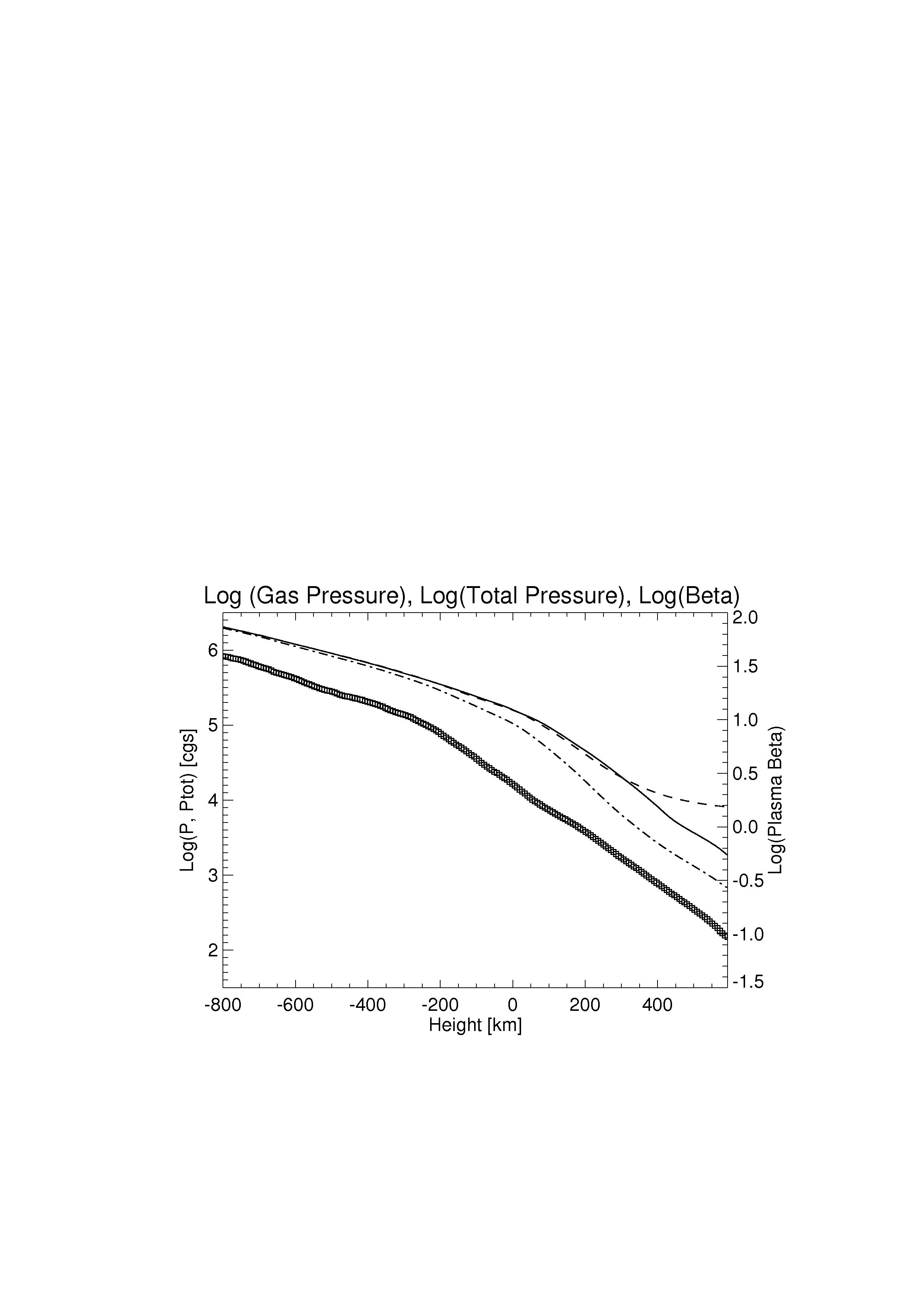
Figure 2: Horizontal average of the plasma $\beta$, gas pressure and total pressure as a function of height. Plotted are, the logarithmic values of the gas pressure averaged over regions with field strength smaller than 50 G (full line), the gas pressure averaged in magnetic flux concentrations (dash-dotted line), the total pressure over magnetic flux concentrations (dashed line) and the plasma $\beta$ (squares; scale on the right).

The total pressure balance between a magnetic flux concentration and its non-magnetic surroundings results from the continuity of the normal stress at the boundary separating the flux concentration from its surroundings. In the $0^{th}$-order approximation (Eq 11), $P_{tot}$ not only matches the boundary value but is also constant across the flux concentration. The presence of $2^{nd}$-order terms (or higher-orders) produces higher or lower values of $P_{tot}$ at the center of flux concentrations (Eq 12) in comparison to $P_{tot}$ at the magnenic/non-magnetic boundary, which remains equal to the external pressure. Thus the total pressure can be used as diagnostic for determining whether a flux concentration has $0^{th}$ or higher-order configuration. In order to illustrate the distributions of pressures and magnetic field in the simulation box, which includes different sizes and shapes of magnetic concentrations, we show in Figure 3 maps of the gas and total pressures as well as $B_{z}$ at three heights $-98$, $182$ and $462$ km, where the reference height $0$ is roughly situated $-100$ km below the average continuum optical depth unity, $\tau_{5000}=1$.

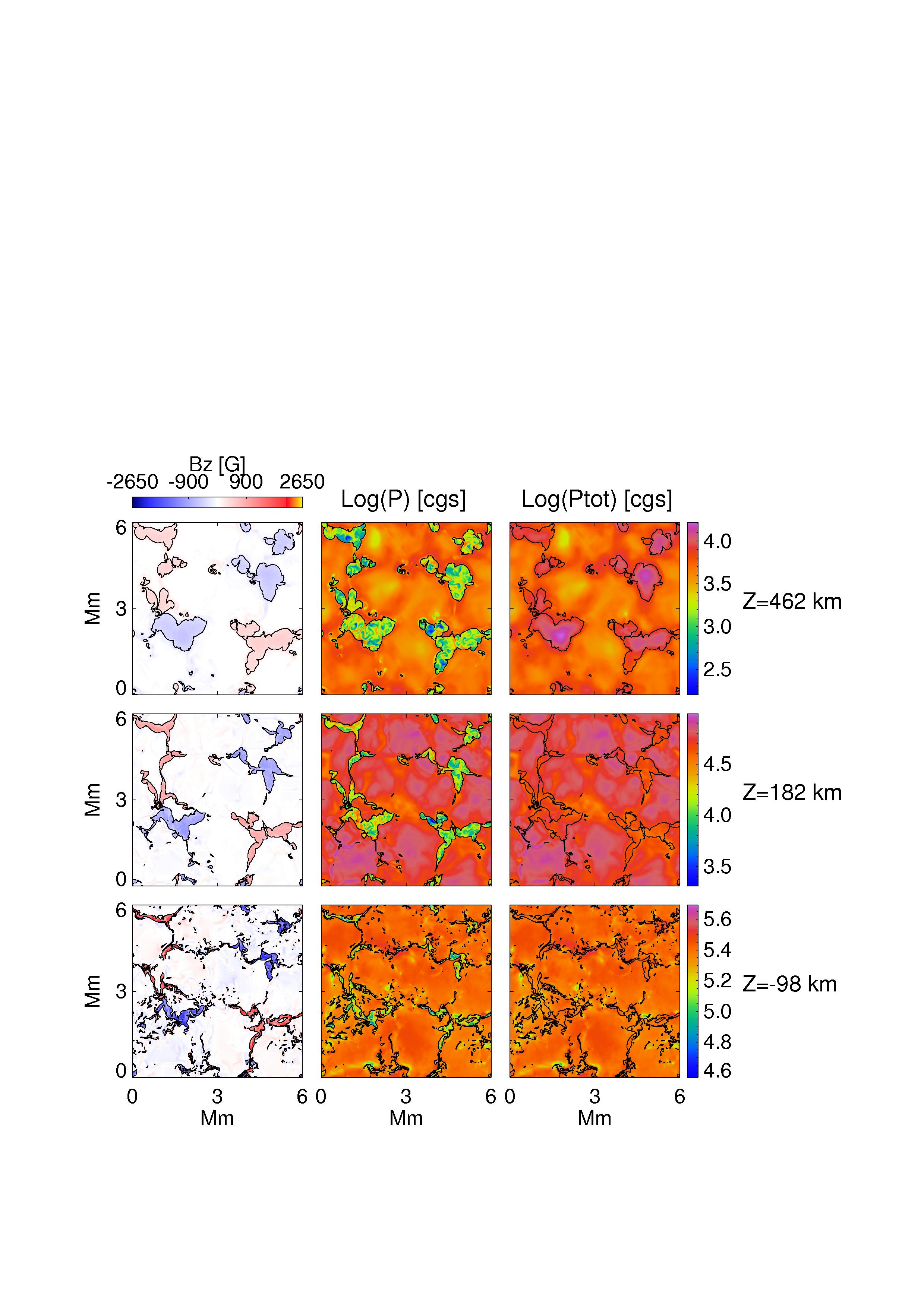
Figure 3: Gas pressure, total pressure and vertical component of the magnetic field at three geometrical heights $-98$, $182$ and $462$ km. The reference height ”$0$” is located at $-100$ km below the average continuum optical depth unity at $5000$ Å. A common color table is used for the three $B_{z}$ maps. At each height, the pressures share the same color table indicated on the right-side of the maps. The black contours enclose regions where $|B_{z}|$ is higher than $500$ G at $-98$ km, higher than $400$ G at $182$ km and higher than $300$ G at $462$ km.

The vertical component of the magnetic field at $-98$km is displayed in the lower left pannel of Figure 3. Note that the flux resides mainly in strong flux concentrations located in intergranular lanes. The middle panel of the lower row in Figure 3 represents gas pressure at $-98$ km. Locations where the magnetic flux density is higher than 500 G are outlined by dark contours. The gas pressure is higher at centers of granules comparing to intergranules. This pressure excess drives the horizontal flows towards the intergranular lanes (see e.g. Stein & Nordlund, 2003). Intergranular lanes display a mixed picture with high gas pressure (which stops the horizontal flows) but also low pressure areas. The magnetic flux concentrations show lower gas pressure.

The total pressure inside flux concentrations at $-98$ km (lower right panel of Figure 3) is roughly close to gas pressure outside, and does not vary significantly within individual flux concentrations. Constant $P_{tot}$ is a necessary condition (but not sufficient) for the validity of the $0^{th}$-order thin flux tube/sheet model.

The existence of $2^{nd}$-order terms (or higher-orders) in pressure and magnetic field leads to higher/lower values of the total pressure at the center of flux concentrations. So, one way of measuring the importance of higher-order terms is to compute the standard deviation and the mean value of the total pressure inside magnetic elements and compare them with the corresponding values outside magnetic regions (see Table 1).

Table 1: Standard deviations and mean value of $P_{tot}$

Altitude [km]	-98	182	462
Standard deviation of $P_{tot}$ in non-magnetic regions ($\sigma_{NM}$) [cgs]	27703.0	9707.59	1055.04
Standard deviation of $P_{tot}$ in magnetic regions ($\sigma_{M}$) [cgs]	32709.4	7950.80	2151.41
Mean value of $P_{tot}$ in non-magnetic regions ($\overline{NM}$) [cgs]	254220.0	57750.9	4901.33
Mean value of $P_{tot}$ in magnetic regions ($\overline{M}$) [cgs]	249696.0	47409.8	8626.20
$\sigma_{NM}$/$\overline{NM}$	0.108	0.168	0.215
$\sigma_{M}$/$\overline{M}$	0.130	0.167	0.249

At an altitude of $-98$ km (Table 1), $\overline{M}$ is slightly lower than $\overline{NM}$ because magnetic flux concentrations are located in intergranular lanes where the pressure at this altitude is slightly lower than the average pressure over the simulation domain. $\sigma_{M}$/$\overline{M}$ is larger than $\sigma_{NM}$/$\overline{NM}$, this does not result from higher-order terms, but rather indicates the presence of fluctuations inside magnetic elements. This is due to the fact that the plasma beta at this altitude is larger than unity (See Fig. 2) which indicates that convection affects and perturbs the field’s regularity. Note that locations with particularly low total pressure (e.g. the green-colored ones) are generally unrelated to magnetic flux concentrations.

At a higher altitude ($182$ km) we see in Figure 3 that magnetic structures have expanded. The gas pressure has, on average, lower values in intergranular lanes and particularly low values inside magnetic elements. The total pressure is lower in intergranular lanes even when there is no (or low) magnetic field, e.g. in the region around the coordinates (3Mm, 2.8Mm). The mean value $\overline{NM}$ is higher than $\overline{M}$ (Table 1). The normalized fluctuations of $P_{tot}$ inside and outside magnetic elements are similar ($\sigma_{M}$/$\overline{M}$$\approx$$\sigma_{NM}$/$\overline{NM}$). Hence there is little evidence for a significant contribution from higher-order terms.

Near the top of the box, at a geometrical height of $462$ km, we notice that the total pressure (Figure 3) increases towards the center of flux concentrations. $\overline{M}$ $>$ $\overline{NM}$ and $\sigma_{M}$/$\overline{M}$ $>$ $\sigma_{NM}$/$\overline{NM}$. This indicates that the total pressure is not a $0^{th}$-order function. This effect is more pronounced in large flux concentrations. The plasma $\beta$ is small at these heights (see Fig. 2), thus we expect a nearly force-free equilibrium with a balance between curvature force and magnetic pressure gradient. So the outward magnetic pressure force will be balanced by the inward curvature force. Thus the magnetic pressure ($\simeq$ total pressure) has to increase inward. Hence the increase of $P_{tot}$ at the center of flux concentrations in the upper right panel of Figure 3.

5 Analysis of individual magnetic structures

The flat profiles of total pressure in the lower part of the atmosphere are in favour of the applicability of the $0^{th}$-order thin flux tube/sheet approximation. In the upper part of the atmosphere, however, the magnetic features show a total pressure excess in their center. This indicates that the $0^{th}$-order thin flux tube/sheet approximation is not applicable, but possibly the extension of the approximation to $2^{nd}$-order is sufficient to describe the force equilibrium of the magnetic structures. For a quantitative investigation we select three flux concentrations in the MHD simulation run according to their width and morphology. These will be treated in the next three sub-sections.

5.1 Thin flux sheet

We compare the properties of a narrow flux sheet in the MHD simulation (Fig. 1) with the thin flux sheet model presented in Sect. 2.2. Note that the flux tubes/sheets in a magneto-convection simulation are not static (unlike the assumption made in Sect. 2). They interact with the external plasma, and get distorted by the granulation motion. They also exchange energy (mainly by radiation) with the surroundings. In order to maintain the numerical stability of the simulation, the gradient of any physical quantity cannot be too large between two neighbouring grid cells. More specifically, the magnetic flux density must not jump abruptly from the boundary of a flux tube to the neighbouring non-magnetized plasma (Vögler, 2003). Thus the boundary layer separating a flux tube from the surrounding non-magnetized plasma is a few grid points wide, unlike the tangential discontinuity in the case of an ideal flux tube. We wish to see whether simulations and thin flux sheet/tube approximation are consistent with each other in spite of the fact that MHD flux tubes/sheets have finite boundary layers, internal and external dynamics and deviate from an axi- or translationally symmetric configuration.

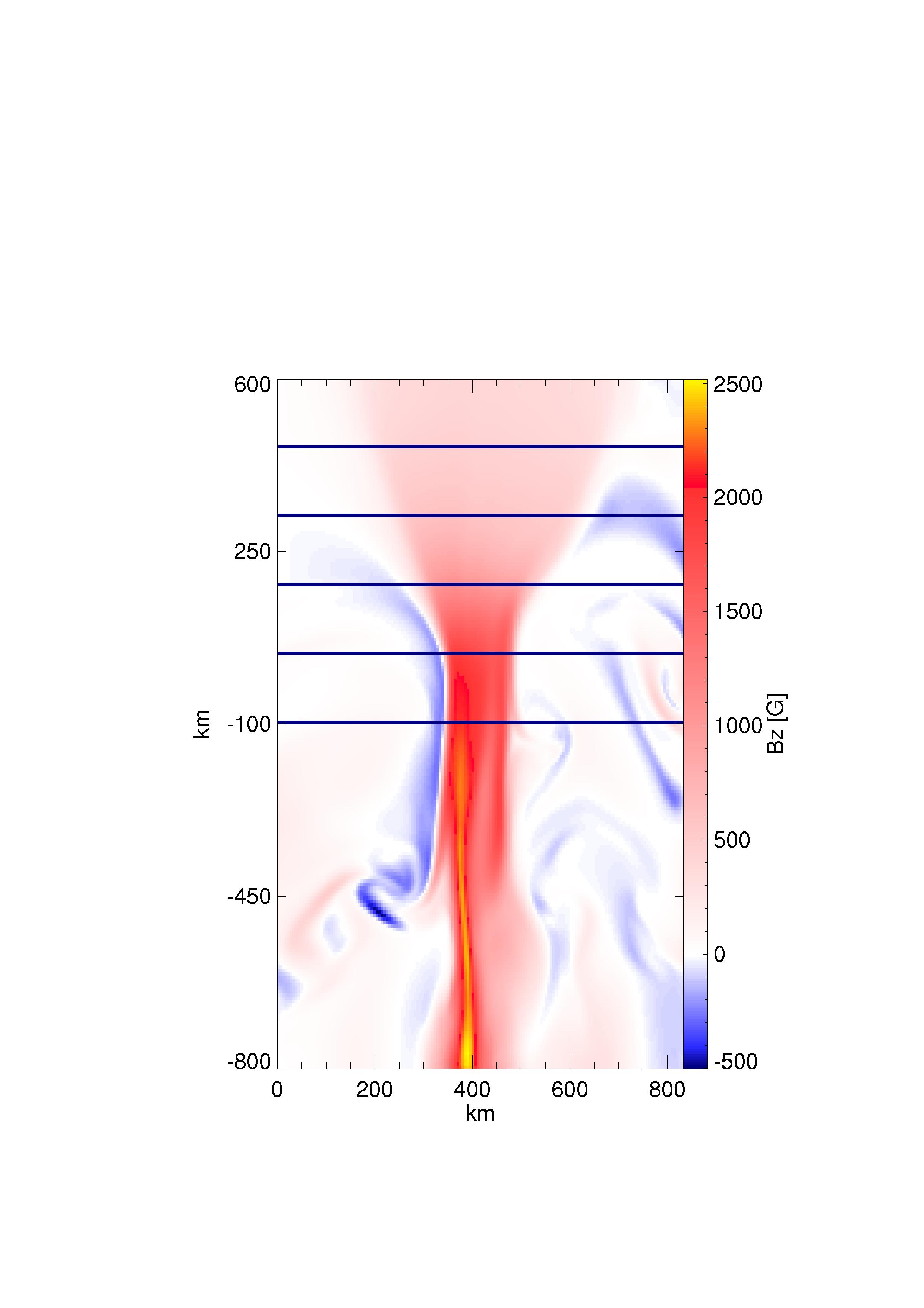
Figure 4: Vertical 2D cut through the MHD simulation box at the location shown by the black line at the upper-left corner in Figure 1. The horizontal lines indicate locations at which we plot profiles of various physical quantities in Figs. 5 to 7.

We select a rather narrow sheet-like structure in the simulation domain. A vertical 2D cut through the flux sheet (shown in Fig. 4) at the location indicated by the dark line in the upper left corner of Fig. 1 reveals the morphology of the magnetic field. The expansion of the flux sheet with height is mainly determined by magnetic flux conservation with height and a horizontal balance between the magnetic plus gas pressure inside the sheet with the gas pressure outside.

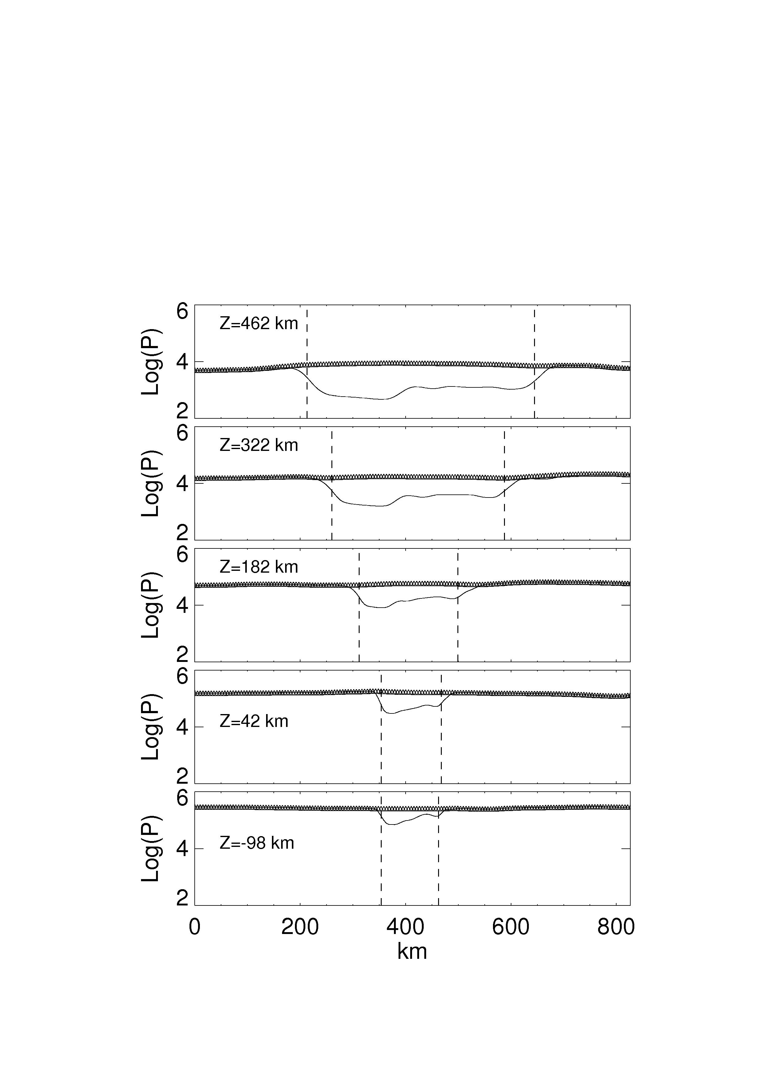
Figure 5: Gas pressure (solid lines) and total pressure (triangles) along the 5 horizontal lines in Figure 4. The vertical dashed lines outline regions where $B_{z}$ is larger than $75$ percent of its maximum value.

Figure 5 shows profiles of gas pressure (full lines) and total pressure (triangles) along the $5$ horizontal lines in Figure 4. The location of the magnetic flux concentration is reflected by the lower gas pressure. The vertical dashed lines outline regions where $B_{z}$ is higher than $0.75$ of its maximum value. The profiles indicate that the flux sheet’s equilibrium in the lower panels is consistent with balance of total pressure in the zeroth-order thin flux sheet approximation (see Eq 11, which is valid for both flux tubes and flux sheets). In the top panel we see that the total pressure increases somewhat towards the center of the sheet, which indicates the necessity of extending the approximation to second- (or higher-) order (see Eq 12). At this height, the plasma $\beta$ has become so small that the internal equilibrium becomes nearly force free, i.e., curvature forces and magnetic pressure gradient balance each other.

Figure 6 shows the vertical component of the magnetic field along the 5 horizontal lines in Figure 4. The triangles represent $B_{z}$ in the case of a thin flux sheet in the second-order approximation. The solid curves represent $B_{z}$ from the MHD simulations. We note that $B_{z}$ for the thin flux sheet at the two lower panels is close to a constant (small contribution from the $2^{nd}$-order terms), whereas in the three upper panels the second-order terms become more important.

The $2^{nd}$-order approximation reproduces reasonably well the overall $B_{z}$ profiles obtained from the MHD simulations in the higher layers of the atmosphere. The profiles of $B_{z}$ from the simulation exhibit some structures across the sheet’s cross-section which are not reproduced by the thin sheet model. This is because this latter model produces only symmetric profiles of $B_{z}$ (Ferriz-Mas & Schüssler, 1989). The actual profiles of $B_{z}$ are asymmetric primarily in the sense that the left part exhibits larger values than the right part. This is associated with lower values of the pressure at these locations, so $B_{z}$ has to increase in order to keep $P_{tot}$ balanced (see Figure 5).

The distribution of the horizontal field component and its approximation with the thin flux sheet model are shown in Fig. 7. Here $B_{x}$ includes a third-order term (see section 2.2). The profiles of the actual field are smooth for the three upper panels (low $\beta$). In the two lowest panel we notice some fluctuations mainly due to perturbations by the external convection. The fit between the simulation result and the thin sheet model is relatively good for the three upper panels, and less good for the two lower ones. We notice that for the three upper panels there is a systematic offset between the actual values and the thin sheet model. This is due to the fact that the sheet is slightly inclined towards the right (more positive $B_{x}$ than negative in Fig. 7). This can also be seen in Fig. 4 at heights above $\approx 150$ km.

$B_{z}$ and $B_{x}$ for the thin flux sheet can be written in a dimensional way (see also Eqns 1 and 2):

$$B_{z}=B_{z0}+x^{2}B_{z2}+x^{4}B_{z4}+...=B0+B2+B4+...,$$ (16)

$$B_{x}=xB_{x1}+x^{3}B_{x3}+...=B1+B3+...,$$ (17)

We can compare the relative importance of successive terms in these series expansions. Table 2 indicates that the average values $\overline{|B2|}$ are significantly smaller than $\overline{|B0|}$. The importance of $\overline{|B2|}$ is more pronounced in the upper part of the atmosphere. This is also noticeable in the upper panels of Figure 6. In a similar way to Sect. 2.2 we calculate $4^{th}$-order terms (see also Pneuman et al. (1986) and Ferriz-Mas & Schüssler (1989)). Table 2 shows that $\overline{|B4|}$ terms are very small compared to $\overline{|B0|}$. Their relative importance reaches its maximum in the top part of the atmosphere, though they remain negligible in practical terms. Similarly, $\overline{|B3|}$ terms are very much smaller than $\overline{|B1|}$. Thus the influence of successive terms in Eqs. (16) and (17) decrease with their order. This is clearly seen in Figures 6 and 7, and confirms that neglecting the $4^{th}$-order terms in $B_{z}$ is justified.

Table 2: Relative importance of the average values of the series expansion $\overline{|B2|}$/$\overline{|B0|}$, $\overline{|B4|}$/$\overline{|B0|}$ and $\overline{|B3|}$/$\overline{|B1|}^{\mathrm{*}}$.

Thin flux sheet: height from reference [km]	-98	42	182	322	462
$\overline{|B2|}$/$\overline{|B0|}$	0.009	0.014	0.036	0.118	0.106
$\overline{|B4|}$/$\overline{|B0|}$	7.67 e-05	2.75 e-05	0.001	0.010	0.015
$\overline{|B3|}$/$\overline{|B1|}$	0.086	0.028	0.006	0.056	0.035
Thick flux tube: height from reference [km]	-98	42	182	322	462
$\overline{|B2|}$/$\overline{|B0|}$	0.112	0.149	0.007	0.086	0.059
$\overline{|B4|}$/$\overline{|B0|}$	0.017	0.012	4.75 e-04	0.011	0.003
$\overline{|B3|}$/$\overline{|B1|}$	0.183	0.142	0.094	0.023	0.034

• Vertical bars indicate absolute values and overlines indicate horizontal average over the sheet’s cross-section

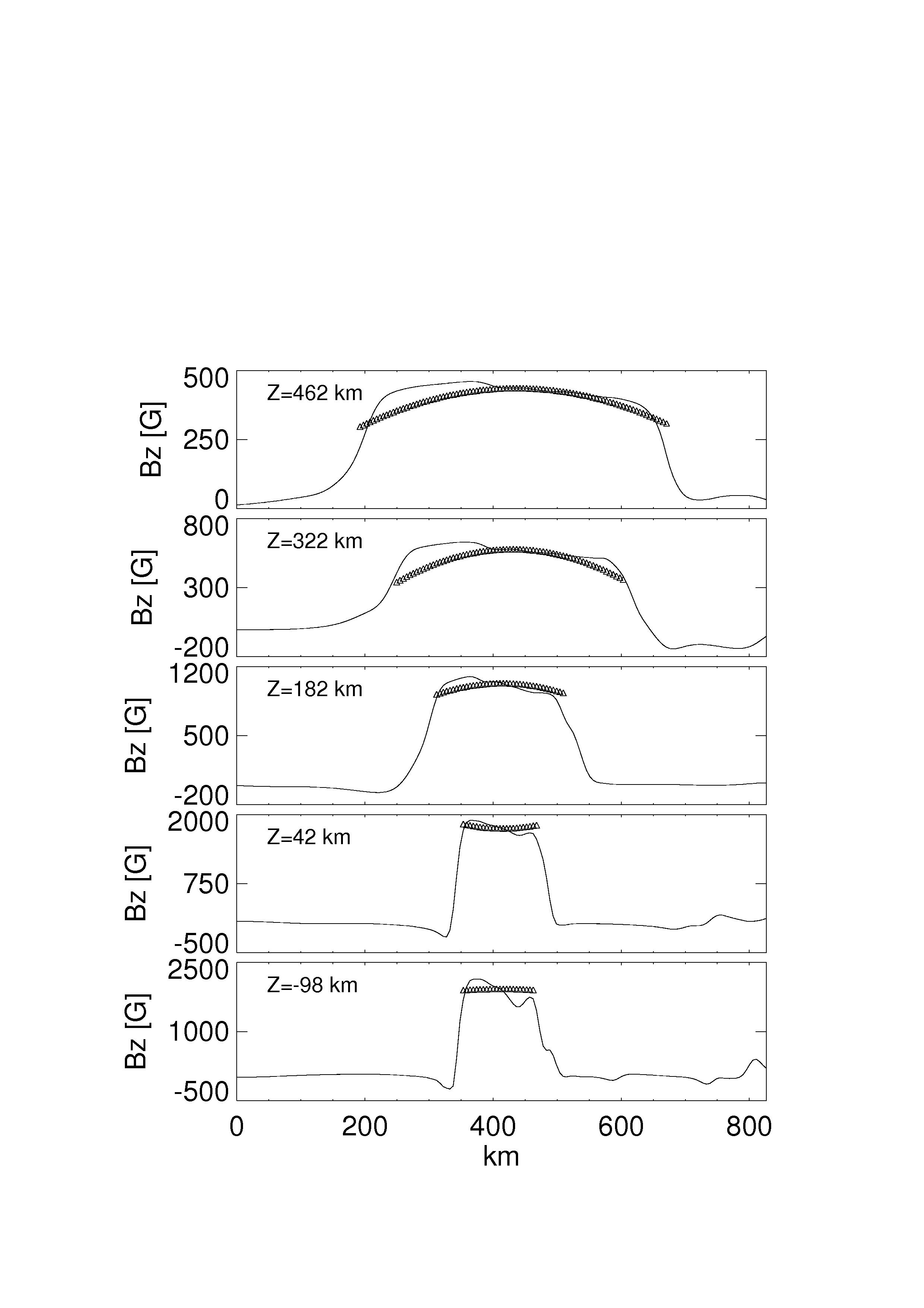
Figure 6: Vertical component of the magnetic field, $B_{z}$, along the $5$ horizontal lines in Figure  4 (solid lines). The triangles represent $B_{z}$ resulting from a $2^{nd}$-order thin flux sheet model.

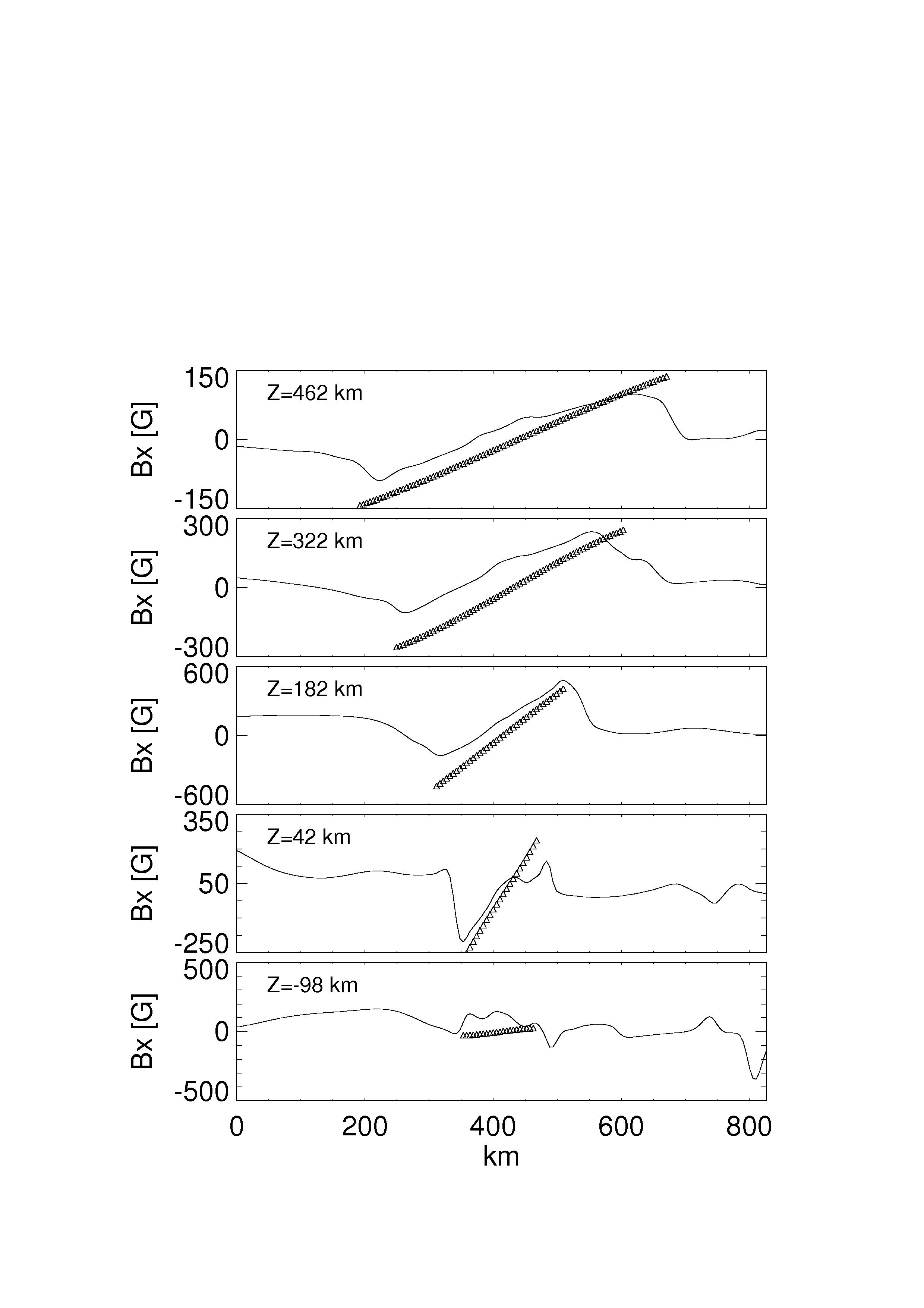
Figure 7: Full lines: horizontal component of the magnetic field, $B_{x}$, across the flux sheet plotted along the $5$ horizontal cuts in Fig. 4. The triangles represents $B_{x}$ resulting from a $2^{nd}$-order thin flux sheet model.

5.2 Analysis of a broad flux concentration

In this section, we compare $B_{z}$ and $B_{r}$ from a thick flux concentration with the thin tube model (Sect. 2.1). The criteria for the choice of a flux tube in the MHD simulations are primarily its width and a relative smoothness of $P_{tot}$ across it. The selected flux tube is located in the lower right part of Fig. 1 (crossed by a dark line). The first thing to note is that the tube is split near the solar surface, which probably results from the history of its interaction with convection. We also notice that this ”tube” has a cross-section which deviates significantly from a circular area (see Fig. 1).

Inspite of these facts, the thin flux tube model reproduces reasonably well the overall shape of $B_{z}$ given in the three upper panels of Fig. 8. In the upper two, we notice the existence of a region with smoother decrease of $B_{z}$ at the left edge of the flux tube. This results from a small neighbouring magnetic structure that merges with the main flux tube. This structure is not visible in the lower panels since at those heights it does not overlap the dark line (Fig. 1). It appears at the highest panels because its expansion with height makes it reach the location of the cut in the MHD cube. We don’t aim to reproduce this neighbouring structure, but only the main flux tube.

In the deeper layers of the photosphere (lower panels of Fig. 8) the relatively thick flux tube splits down its center into two parts. The two separate parts of the flux tube in the lower photosphere merge while expanding with height. It is interesting that such groups of flux concentrations tend to behave like a single flux tube higher up in the atmosphere owing to expansion and the decrease of $\beta$ with height.

The splitting of the flux tube in the lowest panel leads to a decrease of the horizontally averaged field strength at this height compared to the second-lowest panel. It is seen in the framework of the thin flux tube model as an expansion of the flux tube with depth and produces positive values of $h_{2}$ (Eq. 6), clearly seen in the lowest panel.

The radial component of the magnetic field fits reasonably well with the thin flux tube model for the three upper panels (Fig. 9), except at the left edge where the small magnetic feature has merged with the main flux tube. In the two lower panels the actual profiles of $B_{r}$ are disturbed by the double structure of the flux tube. In this case the thin flux tube model cannot be expected to reproduce the actual profiles. In the lowest panel, $B_{r}$ from the thin flux tube model has a negative slope due to the expansion of the flux tube with depth, which leads to negative values of $f_{1}$ (Eq. 7).

The $4^{th}$-order terms remain very small at all altitudes compared to lower orders (Table 2). At the three upper altitudes, the $3^{rd}$-order contribution is clearly less marked than the $1^{st}$-order one. The uneven flux distribution at the two lower altitudes results in somewhat higher contributions of the $2^{nd}$-, $3^{rd}$- and $4^{th}$- orders compared to the situation at higher altitudes.

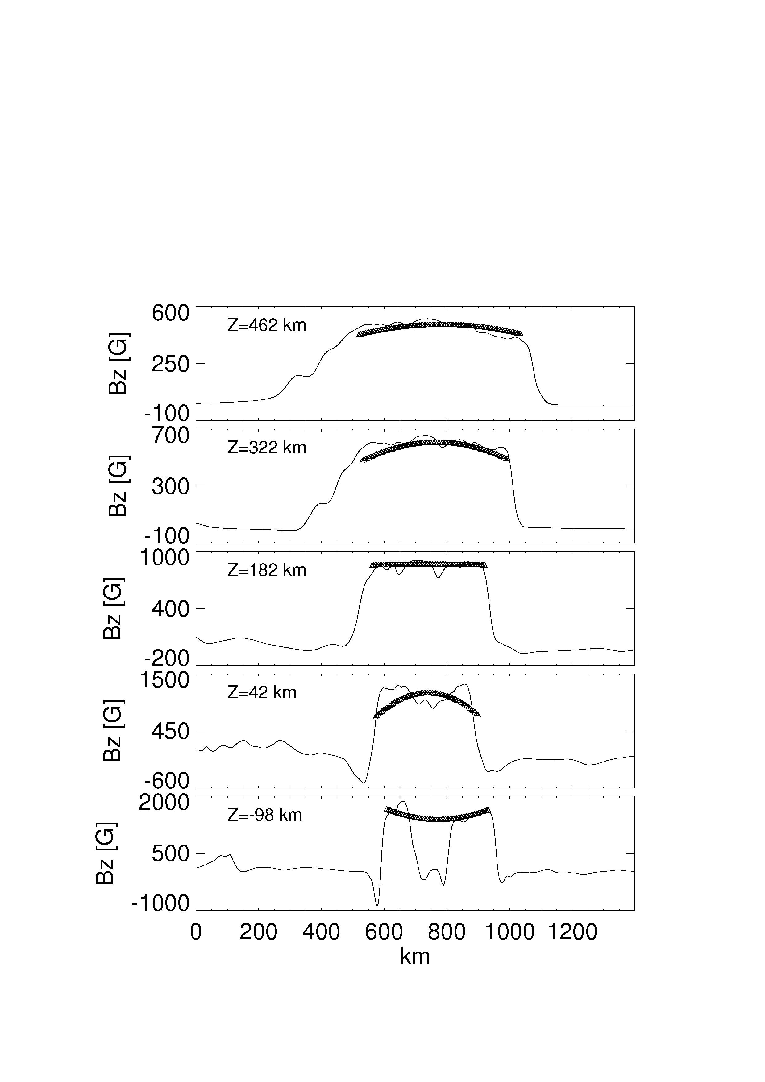
Figure 8: Vertical component of the magnetic field of a thick flux tube in the MHD snapshot (solid lines) along the black line in the lower right corner of Fig. 3. The triangles represent $B_{z}$ resulting from the thin flux tube model. The 5 plots correspond to the same heights as in Fig. 6.

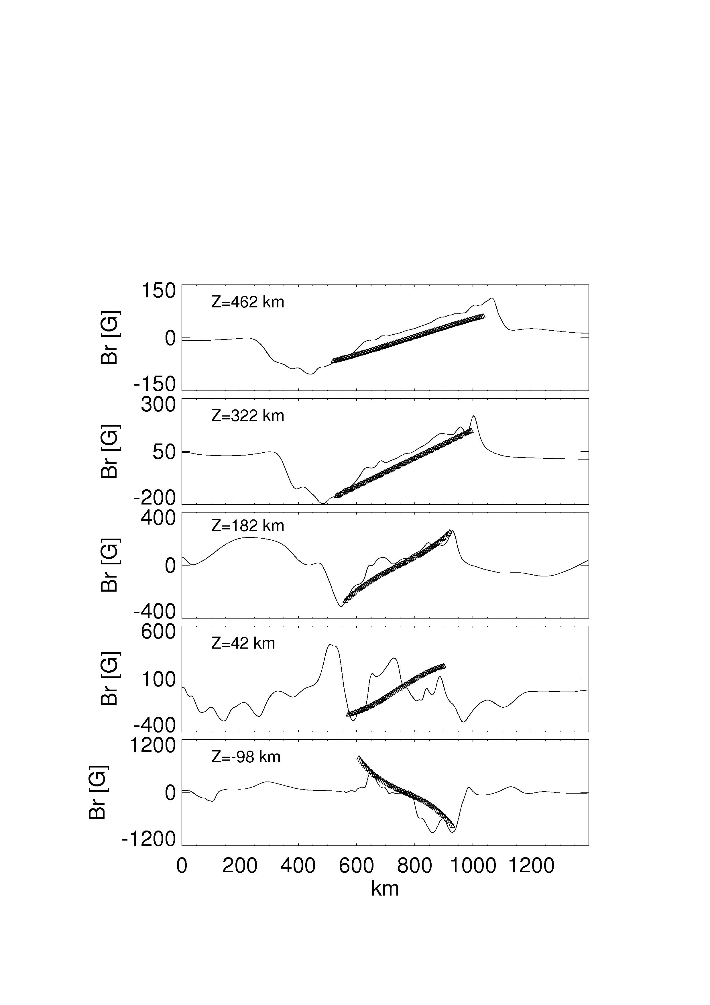
Figure 9: Radial component of the magnetic field across the dark line in the lower right corner of Fig. 3. Solid lines represent $B_{r}$ from the simulation, and triangles are from the thin flux tube model.

5.3 Very thin flux concentration

The thin flux tube/sheet model is generally thought to be best suited to describe the smallest flux concentrations in the MHD simulations. This picture is appropriate for the ideal case where flux tubes/sheets have an extremely thin boundary layer (separating magnetic and non-magnetic regions) and for a static plasma. The situation in the photosphere is clearly different. There vigorous convective flows induce considerable distortions of very thin flux concentrations. As a consequence, the shape and flux density distribution of the thinnest magnetic elements may differ significantly from a thin flux tube/sheet model.

In order for a flux concentration to evolve as a coherent structure in a plasma with density $\rho$ and velocity $V$, its magnetic energy density ($B^{2}/(8\pi)$) has to be larger than the kinetic energy density of the flow ($0.5\rho V^{2}$). In other words, the magnetic field has to be such that $B>B_{eq}=V\sqrt{4\pi\rho}$, where $B_{eq}$ is the equipartition field strength.

At the surface of the sun we have $B_{eq}\simeq 500$ G. This is a limit below which we cannot expect to obtain a structure coherent enough to be described by the thin flux tube/sheet model. Thus we only consider thin magnetic features with $B>B_{eq}>500$ G (see contours on Fig. 1). We also require that flux concentrations remain coherent at higher altitude (see top-left panel in Fig. 3) and are not located in a region close to opposite-polarity fields, since at these locations the field morphology gets complicated.

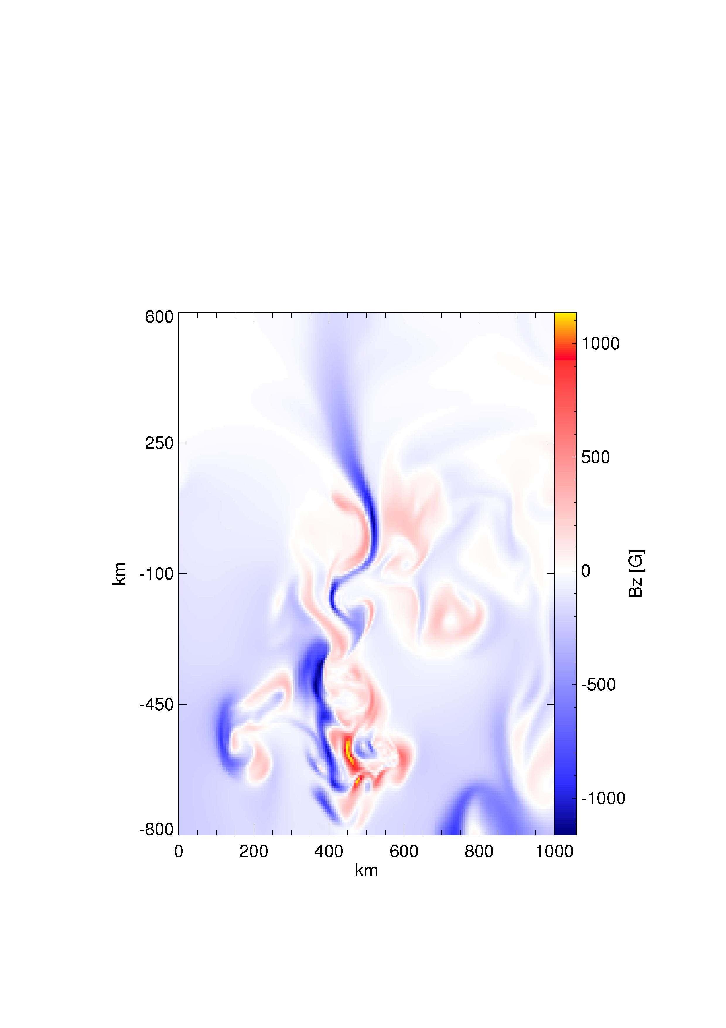
Figure 10: Vertical 2D cut in the MHD data showing $B_{z}$ at the location indicated by the black line in the upper right part of the maps in Fig. 1.

The $B_{z}$ map in the upper left panel of Fig. 3 indicates that only relatively few very-thin flux concentrations (that have not merged with larger magnetic features) are noticeable at the greatest height. We select one of them, at the location shown by the black vertical line in the upper-right part of the maps in Fig. 1.

A lateral 2D view of this thin structure (Fig. 10) shows that it is asymmetric and distorted, with an inclination that varies strongly with height. Since the magnetic energy density is not far above the equipartition value, the convective flows influence the morphology of the thin flux concentration rather strongly. This does not favour of the representation of very thin flux concentrations in terms of thin flux tube/sheet models.

6 Conclusions

The total pressure diagnostic (Sect. 4) indicates that $P_{tot}$ is nearly constant across most flux concentrations near the solar surface. This is a necessary condition for applying the $0^{th}$-order thin flux tube/sheet approximation. In the higher parts of the atmosphere, tension forces become important due to the curved field lines and low plasma $\beta$. In this case, higher orders in the thin flux tube/sheet model are needed to describe flux elements.

For a detailed analysis of magnetic features in the MHD simulation, we have adopted two models (thin flux tube and thin flux sheet) depending on the geometry of the studied flux concentration. We have seen that for flux concentrations with magnetic field well above the equipartition distribution (Sects 5.1 and 5.2), the models reproduce reasonably well $B_{z}$ and $B_{x}$ (or $B_{r}$) of the simulated flux concentrations. This was especially the case in the higher part of the atmosphere. The fits were less good in the lower part of the atmosphere due to higher $\beta$ and the vigorous convective flows. In this case, it is rather the overall shape of $B_{z}$ that is consistent with the approximation. The $2^{nd}$-order terms of the thin flux tube/sheet approximation contribute at the $5$-$15$ percent level especially in the upper part of the atmosphere. The $3^{rd}$-order terms provide a relatively small contribution to $B_{x}$ or $B_{r}$, while the $4^{nd}$-order terms give a very small contribution to $B_{z}$. This justifies neglecting the $4^{th}$-order terms and the view that higher-orders contribute less and less to $B_{z}$ and $B_{x}$ (or $B_{r}$).

In the case of very thin flux concentrations which generally have energy densities lower than or at most somewhat higher than the equipartition value, field lines are distorted and partly driven by plasma motions. This leads to distorted or incoherent flux concentrations which do not have the necessary symmetry and regularity to be reproduced by a thin flux tube/sheet model. To what extent these low field strengths are due to the limited resolution (low Reynold’s number) of the simulations still needs to be established. Note, however, that it has been pointed out (Venkatakrishnan, 1986) that the convective collapse mechanism, thought to be responsible for the concentration of magnetic flux to kG strengh (Parker, 1978; Spruit, 1979; Grossmann-Doerth et al., 1998), becomes less efficient as the amount of magnetic flux per feature decreases. A decrease in field strength with decreasing magnetic flux has been observationally confirmed (Solanki et al., 1996).

Acknowledgements: This work was partly supported by the WCU grant No. R31-10016 from the Korean Ministry of Education, Science and Technology. L.Y.C. is thankful to the Max-Planck-Institut f r Sonnensystemforschung, Katlenburg-Lindau for a stipend of the International Max Planck Research School on Physical Processes in the Solar System and Beyond.

References

- Bercik (2002) Bercik, D. J. 2002, PhD thesis, Michigan state university
- Bruls & Solanki (1995) Bruls, J. H. M. J. & Solanki, S. K. 1995, A&A, 293, 240
- Defouw (1976) Defouw, R. J. 1976, ApJ, 209, 266
- Ferriz-Mas & Schüssler (1989) Ferriz-Mas, A. & Schüssler, M. 1989, Geophysical and Astrophysical Fluid Dynamics, 48, 217
- Ferriz-Mas et al. (1989) Ferriz-Mas, A., Schüssler, M., & Anton, V. 1989, A&A, 210, 425
- Grossmann-Doerth et al. (1998) Grossmann-Doerth, U., Schüssler, M., & Steiner, O. 1998, A&A, 337, 928
- Martínez Pillet et al. (1997) Martínez Pillet, V., Lites, B. W., & Skumanich, A. 1997, ApJ, 474, 810
- Nordlund (1983) Nordlund, A. 1983, in IAU Symposium, Vol. 102, Solar and Stellar Magnetic Fields: Origins and Coronal Effects, ed. J. O. Stenflo, 79–83
- Nordlund & Stein (1990) Nordlund, Å. & Stein, R. F. 1990, in IAU Symposium, Vol. 138, Solar Photosphere: Structure, Convection, and Magnetic Fields, ed. J. O. Stenflo, 191
- Parker (1978) Parker, E. N. 1978, ApJ, 221, 368
- Pneuman et al. (1986) Pneuman, G. W., Solanki, S. K., & Stenflo, J. O. 1986, A&A, 154, 231
- Rabin (1992) Rabin, D. 1992, ApJ, 391, 832
- Roberts & Webb (1978) Roberts, B. & Webb, A. R. 1978, Sol. Phys., 56, 5
- Roberts & Webb (1979) Roberts, B. & Webb, A. R. 1979, Sol. Phys., 64, 77
- Rüedi et al. (1992) Rüedi, I., Solanki, S. K., Livingston, W., & Stenflo, J. O. 1992, A&A, 263, 323
- Schüssler (1992) Schüssler, M. 1992, in NATO ASIC Proc. 373: The Sun: A Laboratory for Astrophysics, ed. J. T. Schmelz & J. C. Brown, 191
- Solanki (1993) Solanki, S. K. 1993, Space Science Reviews, 63, 1
- Solanki et al. (2006) Solanki, S. K., Inhester, B., & Schüssler, M. 2006, Reports on progress in physics, 69, 563 668
- Solanki et al. (1996) Solanki, S. K., Zufferey, D., Lin, H., Rueedi, I., & Kuhn, J. R. 1996, A&A, 310, L33
- Spruit (1979) Spruit, H. C. 1979, Sol. Phys., 61, 363
- Spruit (1981) Spruit, H. C. 1981, A&A, 102, 129
- Stein & Nordlund (1998) Stein, R. F. & Nordlund, A. 1998, ApJ, 499, 914
- Stein & Nordlund (2003) Stein, R. F. & Nordlund, Å. 2003, in Astronomical Society of the Pacific Conference Series, Vol. 288, Stellar Atmosphere Modeling, ed. I. Hubeny, D. Mihalas, & K. Werner, 519
- Stenflo (1973) Stenflo, J. O. 1973, Sol. Phys., 32, 41
- Venkatakrishnan (1986) Venkatakrishnan, P. 1986, Nature, 322, 156
- Vögler (2003) Vögler, A. 2003, PhD thesis, Universität Göttingen
- Vögler & Schüssler (2003) Vögler, A. & Schüssler, M. 2003, Astronomische Nachrichten, 324, 399
- Vögler et al. (2005) Vögler, A., Shelyag, S., Schüssler, M., et al. 2005, Astron. & Astrophys., 429, 335
- Wiehr (1978) Wiehr, E. 1978, Mitteilungen der Astronomischen Gesellschaft Hamburg, 43, 134
- Zayer et al. (1989) Zayer, I., Solanki, S. K., & Stenflo, J. O. 1989, A&A, 211, 463