Spin-waves in the $J_{1a}-J_{1b}-J_{2}$ orthorombic square-lattice Heisenberg models: Application to the iron pnictide materials

Abstract

Motivated by the observation of spatially anisotropic exchange constants in the iron pnictide materials, we study the spin-wave spectra of the $J_{1a}-J_{1b}-J_{2}$ Heisenberg models on a square-lattice with nearest neighbor exchange $J_{1a}$ along x and $J_{1b}$ along y axis and a second neighbor exchange $J_{2}$. We focus on the regime, where the spins order at ($\pi,0$), and compute the spectra by systematic expansions around the Ising limit. We study both spin-half and spin-one Heisenberg models as well as a range of parameters to cover various cases proposed for the iron pnictide materials. The low-energy spectra have anisotropic spin-wave velocities and are renormalized with respect to linear spin-wave theory by up to 20 percent, depending on parameters. Extreme anisotropy, consisting of a ferromagnetic $J_{1b}=-|J_{F}|$, is best distinguished from a weak anisotropy ($J_{1a}\approx J_{1b}=J_{1}$, $J_{2}>J_{1}/2$ ) by the nature of the spin-waves near the wavevectors ($0,\pi$) or ($\pi,\pi$). The reported spectra for the pnictide material CaFe₂As₂ clearly imply such an extreme anisotropy.

The parent phases of iron pnictide superconductors have been found to be metallic but with antiferromagnetic order at low temperatures.kamihara ; cruz ; dong There is an ongoing debate between the validity of a strong-coupling picture, with local spins interacting via Heisenberg exchange interactions, and a weak coupling picture where partial nesting of the fermi-surface leads to a spin-density-wave order.yin ; cao ; ma ; yildrim ; wu ; haule ; si ; yao ; xu ; mazin ; raghu ; ran ; baskaran ; han ; rajiv ; chen In this paper we will not get into this debate but rather focus on the systematic calculations of spin-wave spectra for Heisenberg models on an anisotropic square-lattice with nearest and second neighbor interactions, using series expansion methods.book ; advphy Such studies of spatially anisotropic interactions on triangular-lattices have proved fruitful in understanding magnetic properties of several organic and inorganic materials.coldea1 ; coldea2 This work should similarly be helpful for understanding materials with an orthorombic square-lattice geometry.pardini

Neutron scattering spectra for the pnictides show sharp spin-waves.zhao1 In the low temperature phase there is orthorombic distortion and the exchange constants have been found to be substantially anisotropic. For different materials, and sometimes even for the same material, different exchange constants have been reported.zhao ; broholm In some cases, there are reports of extreme anisotropy in the nearest-neighbor exchange. They are found to be strong and antiferromagnetic along one axis and weak and ferromagnetic along the other.zhao The origin of the strong spatial anisotropy remains controversial, one theory being that it is due to orbital order,frank ; yildrim2 ; rajiv ; chen ; ashvin ; weiku which may drive the tetragonal to orthorombic transition in these materials. In this paper, we focus on temperatures much below the ordering temperature, where in the strong coupling picture a Heisenberg Hamiltonian should be appropriate.

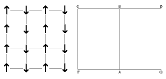
Figure 1: On the left is the ordering pattern of the pnictides. On the right is the positive quadrant of the square-lattice Brillouin Zone showing wavevectors $\Gamma$ ($0,0$), $A$ ($\pi/2,0$), $Q$ ($\pi,0$), $D$ ($\pi,\pi$), $B$ ($\pi/2,\pi$) and $C$ ($0,\pi$). With long-range order at ($\pi,0$) the distinct energies are contained inside the region $\Gamma ABC$.

We will consider the Hamiltonian:

$$H= J_{1a}\sum_{i}\vec{S}_{i}\cdot\vec{S}_{i+\hat{x}}+J_{1b}\sum_{i}\vec{S}_{i}\cdot\vec{S}_{i+\hat{y}}$$

$$+J_{2}\sum_{<i,k>}\vec{S}_{i}\cdot\vec{S}_{k},$$

The first two terms represent the nearest-neighbor exchange along the x and y axes respectively. The third term is the second-neighbor exchange which is taken to be independent of direction. Here we are interested in parameter ranges that lead to antiferromagnetic order at ($\pi,0$) as found in the iron pnictides. There are two ranges of parameters of interest: (i) $J_{1a}$ is the largest energy scale, $J_{1b}$ is small positive or negative and $J_{2}$ is of order or smaller than $J_{1}/2$. (ii) $J_{1a}$ and $J_{1b}$ are comparable and $J_{2}>J_{1a}/2,J_{1b}/2$. The latter case is highly frustrated and colinear ($\pi,0$) order is stabilized by quantum fluctuations. In the former case, the system is unfrustrated or weakly frustrated and ($\pi,0$) order minimizes all or nearly all the interactions.

The case of $J_{1a}=J_{1b}$ was discussed in an earlier study.uhrig That case is conceptually more subtle as the classical ground state in the ($\pi,0$) phase is highly degenerate. Spins on the two sublattices of the square-lattice are free to rotate with respect to each other. The colinear order is selected by quantum fluctuations through an order by disorder mechanism.shender ; chandra ; capriotti This also has important consequences for the spin-wave spectra. The linear spin-wave spectra has spurious gapless modes in addition to those required by Goldstone’s theorem. These become gapped upon proper inclusion of quantum fluctuations.uhrig ; singh Once $J_{1a}$ is not equal to $J_{1b}$, the classical ground state becomes unique becoming antiferromagnetic along the direction of larger exchange, and linear spin-wave theory should give the qualitatively correct spectra.

The linear spin-wave dispersion for the model is given byrajiv

$$\omega_{k}=4SJ_{2}\sqrt{(A_{k}^{2}-B_{k}^{2})}$$ (2)

with

$$A_{k}=1+\alpha-\beta+\beta\cos{k_{y}},$$ (3)

and,

$$B_{k}=\cos(k_{x})(\cos(k_{y})+\alpha).$$ (4)

Here, $\alpha=J_{1a}/(2J_{2})$, and $\beta=J_{1b}/(2J_{2})$. The spectral weights associated with the spin-waves is given by the expression

$$S_{k}\propto\sqrt{{(A_{k}-B_{k})\over(A_{k}+B_{k})}}$$ (5)

These lead to spin-wave velocity along $x$ of

$$v_{x}=2S(2J_{2}+J_{1a})$$

and along $y$ of

$$v_{y}=2S\sqrt{(2J_{2}-J_{1b})(2J_{2}+J_{1a})}.$$

For the numerical calculations, it is convenient to set $J_{1a}=1$. The actual energy scale for the material can be deduced by comparing with experiments. Motivated by the experimentally reported parameters,zhao ; broholm we will study five different parameter sets: (i) $J_{1b}=-0.2$, $J_{2}=0.4$, (ii) $J_{1b}=0$, $J_{2}=0.4$, (iii) $J_{1b}=0.2$, $J_{2}=0.4$, (iv) $J_{1b}=0.2$, $J_{2}=0.9$, (v) $J_{1b}=0.8$, $J_{2}=1.4$. In all cases, will calculate spectra for both spin-half and spin-one models to see if the shape of the spectra has any significant spin dependence.

For all these parameters, we develop Ising series expansions for the spin-wave dispersion and their spectral weights. The series are computed to 8-th order and involve a set of 280474 distinct clusters. These are analyzed throughout the zone using series extrapolation methods. These extrapolation methods converge extremely well if one is not too close to ($0,0$) or the ordering wavevector ($\pi,0$). The dispersion must go to zero near these, with a linear in $q$ behavior although with anisotropic spin-wave velocities. We have used the method of Singh and Gelfandsg to calculate the spin-wave velocities. Very near these wavevectors the linear dispersion is assumed with the calculated anisotropic spin-wave velocities to obtain the spectra. The spectral weights are calculated by the methods discussed by Zheng et al.zheng The spectral weights vanish near ($0,0$) but diverge as $1/q$ near the ordering wavevector. We will not focus much on the region very close to this divergence. Away from that point, simple Pade approximants (or just addition of terms in the series) converges very well. We will see that what distinguishes the different models, after an overall energy scale has been scaled out of the problem, is the nature of the high-energy short-wavelength spin-waves and that is our primary focus here.

The spin-wave velocities along x and y for the different parameter ranges calculated from the series expansions are shown in Table I for spin-half and Table II for spin-one. The colinear ordering pattern and the square-lattice Brillouin zone with some q-vectors used for defining the contours along which spectra will be shown are depicted in Fig 1.

Figure 2: Linear spin-wave spectra for the models along selected contours in the Brillouin Zone.

Figure 3: Spin-wave spectra calculated by series expansions for the spin-half models along selected contours in the Brillouin Zone.

Figure 4: Spin-wave spectra calculated by series expansions for the spin-one models along selected contours in the Brillouin Zone.

Figure 5: Spectral weights associated with the spin-waves, in arbitrary units, along a special contour in the momentum space for the spin-half Heisenberg models, as calculated by Ising series expansions.

In Fig 2, Fig. 3, and Fig. 4, we show the calculated spectra along a selected contour in the Brillouin zone for the spin-half model, spin-one model, and linear spin-wave theory respectively. The uncertainties in the series calculations, over most of the Brillouin zone, are of order one percent. Note that within linear spin-wave theory spin-wave dispersion would be independent of spin once an overall energy scale has been taken out. There is a clear overall similiraity between the spectra, showing that spin value does not significantly alter the shape of the spectra. Also, having $J_{1a}$ not equal to $J_{1b}$ clearly improves the validity of spin-wave theory.uhrig The primary correction to linear spin-wave theory is an upward renormalization of the spectra, which is up to $20\%$ for the spin-half case and less than $10\%$ for the spin-one case. Even at low energies these renormalizations are found to be anisotropic. The renormalization of spin-wave energy is especially non-uniform near the antiferromagnetic zone-boundary. Most notably, flat regions of the linear spin-wave spectra acquire some dispersion on inclusion of quantum fluctuations. As expected, these structures are more pronounced for spin-half than for spin-one case. This is not dissimilar to the nearest-neighbor square-lattice case, where also the zone-boundary dispersion acquires a structure that is absent in linear spin-wave theory.sg ; zheng ; sandvik

Figure 6: Spectral weights associated with the spin-waves, in arbitrary units, along a special contour in the momentum space obtained from Linear Spin Wave theory

The spectral-weights associated with the spin-waves for the spin-half models and for linear spin-wave theory are shown in Fig. 5 and Fig. 6 respectively. One finds that along cetrain directions, and especially at long-wavelengths the different models are indistinguishable. The major differences between different parametrs sets arise when one considers the weights at short wavelengths or high energies. In the extreme anisotropy case, when the spin-wave is a maximum at ($0,\pi$), there is only a small scattering intensity around that wavevector. In the weak anisotropy limit, when there is low excitation energies at these wavevectors, there is also enhanced intensity at these wavevectors.

The density of states for the spin-half models are shown in Fig. 7. The key distinguishing feature is that the weakly frustrated models have sharp peaks close to highest energies. This is also evident from the spectra, where there are flat regions in the dispersion curve.

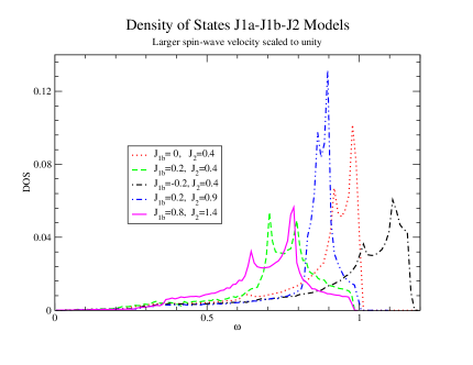
Figure 7: Density of states for the different spin-half models as calculated by series expansions.

We now discuss the relevance of these calculations to the observed spectra in the iron pnictide materials. We first note that the observation of sharp spin-waves throughout the Brillouin zone would be strongly supportive of a local moment picture. Zhao et alzhao have argued that this is indeed the case and that there is an absence of a Stoner continuum in these materials, which should have been present if an itinerant picture for the magnetism was more appropriate. This suggests that magnetism and metallic behavior can be treated separately. This controversial issuetom is clearly beyond the scope of the present work. We will instead restrict ourselves to discussing the spin-wave dispersion and spectral intensities expected from the Heisenberg models in different parameter regimes, so that they can guide future experiments. As discussed earlier, spin does not play a big role in these models except to set the overall energy scale in terms of $J$. However, since $J_{1a}$ is an adjustable parameter, it can always be rescaled to match the experimental data. Hence, all comparisons below are done in terms of the spin-half models.

Figure 8: A comparison of the measured spectra in CaFe₂As₂, with the different models.

Fig. 8, shows a comparison of the calculated dispersion for the different parameters with the experimental measurements in CaFe₂As₂. In all cases, the exchange constant $J_{1a}$ is adjusted to match with the low energy spectra near the zone center. The estimated values for $J_{1a}$ are $86.9$, $86.1$, $86.0$, $58.9$ and $44.3$ meV in the cases (i) through (v) respectively. Note that theoretical error bars are of order one percent. It is clear that all parameters are equally good for describing the zone-center spectra along both x and y axes. The difference really arises when one studies the zone-boundary excitations. In particular the spectra near ($0,\pi$) can only be explained by the parameters $J_{1b}/J_{1a}=-0.2$, $J_{2}/J_{1b}=0.4$. Even if we make $J_{1b}$ zero or slightly positive, we can no longer describe the high energy spectra. The weakly anisotropic models have sharp dips near ($0,\pi$) and hence have no chance of describing the observed spectra. It would be useful to systematically look for the high energy spin-wave spectra in different family of iron pnictide materials to see how universal the high energy spectra is.

To further guide neutron scattering studies in this direction, we create two dimensional scattering intensity profiles in the Brillouin zone at different frequencies. Our results do not include any form-factor effects and unlike experiments have no noise. We use an artificial Gaussian broadening in $\omega$ to mimic finite experimental resolution. Thus we take

$$S(q,\omega)=S(q)\exp{-{(\omega-\omega_{q})^{2}\over\Delta^{2}}}.$$

with a suitably chosen $\Delta$, which we take to be independent of $q$. Here $S(q)$ and $\omega_{q}$ are the spectral intensity and spin-wave frequencies calculated by series expansions. We focus on cases (i) and (v), which correspond to most anisotropic exchanges and least frustrated model and least anisotropic exchanges and most frustrated model respectively.

In Fig. 9 , the intensities are plotted over the full Brillouin Zone for several different frequencies for the models (i) and (v). The evolution from a single bright spot at the zone center at low energies, due to finite resolution, to an ellipse with a hole in the middle at intermediate energies is a standard feature of this type of ($\pi,0$) order. This feature is similar for all parameter sets. There are clear differences, however, even at low frequencies, which should be resolvable with high accuracy data. The plots on the left are more elliptical and those on the right are more circular. As one moves to high energies and excitations move far from the zone center, details of the local Hamiltonian become clearly visible. The two cases shown have vastly different spectra. It should be noted that relative to the zone center, the intensity at higher energies is significantly diminished. At the highest energy shown, excitations are present only in the plots on the left. The plots on the right just show weak vestiges of lower energy excitations due to the assumed finite resolution.

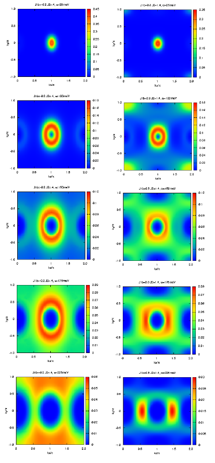
Figure 9: Scattering intensities in the full Brillouin zone centered at the ordering wavevector, for (from top to down) $\omega=$ 25 meV, 100 meV, 150 meV, 175 meV and 225 meV for the strongly anisotropic, weakly frustrated model on the left and weakly anisotropic, strongly frustrated model on the right,

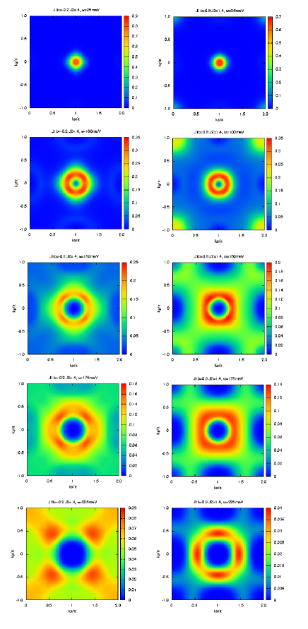
Figure 10: Scattering intensities as in Fig. 9 in a substantially twinned sample, which leads to restoration of tetragonal symmetry

In Fig. 10 intensity plots are made upon averaging the spectra at ($q_{x},q_{y}$) and ($q_{y},q_{x}$), as would be expected in a heavily twinned sample. It is evident that major distinctions between the two models remains evident despite the restoration of the $90$ degree rotational symmetry. So, while the detwinning of the materials may be important to get complete information, spectra from a twinned sample can also distinguish a weakly anisotropic model from a strongly anisotropic one.

In conclusion, in this paper we have used series expansion methods to calculate the spin-wave spectra and spectral weights for orthorombic square-lattice Heisenberg models. We find that the linear spin-wave theory is qualitatively valid for weak and strong frustration. This case is different from a system with tetragonal symmetry where linear spin-wave theory was found to be qualitatively incorrect. In general, the renormalization of the spin-wave energies throughout the zone is of order or less than 20 percent. The high energy spin-waves and their dispersion provide a particularly sensitive way to narrow down parameter ranges and determine the extent of spatial anisotropy in the exchange constants of different orthorombic materials.

The spectra of the iron pnictide materials imply a strongly anisotropic system, where nearest neighbor exchanges are strong and antiferromagnetic in one direction and weak and ferromagnetic in the other. While this study has ignored the metallic nature of the pnictides and focused entirely on a local moment description, the conclusion of strong spatial anisotropy is likely to have much broader validity. The implications of this anisotropy in other properties of the system deserve further attention.

Table 1: [m/n] Pade and overall estimates (Est.) of spin wave velocities ($v_{x},v_{y}$) for spin-half models for different $J_{1b}$ and $J_{2}$ values with $J_{1a}=1.0$

J1b, J2	v	[4/4]	[5/3]	[3/5]	[4/3]	[3/4]	Est.
-0.2, 0.4	vx	2.1029	2.1043	2.1039	2.1013	2.1012	2.10
-0.2, 0.4	vy	1.4162	1.4123	1.4114	1.4056	1.4016	1.41
0.0, 0.4	vx	2.1169	2.1244	1.9803	2.1360	2.1268	2.12
0.0, 0.4	vy	1.2590	1.3712	1.1754	1.2622	1.2619	1.26
0.2, 0.4	vx	2.1120	2.3405	2.1718	2.3117	2.1726	2.19
0.2, 0.4	vy	1.0749	1.1355	1.1092	1.1645	1.1200	1.11
0.2, 0.9	vx	3.1269	3.1532	3.1444	3.1434	3.1410	3.14
0.2, 0.9	vy	2.3616	2.3804	2.3771	2.3816	2.3796	2.38
0.8, 1.4	vx	4.1823	4.3840	4.2505	4.2848	4.2253	4.26
0.8, 1.4	vy	3.2355	3.3711	3.2967	3.4350	3.3278	3.33

Table 2: [m/n] Pade and overall estimates (Est.) of spin wave velocities ($v_{x},v_{y}$) for spin-one models for different $J_{1b}$ and $J_{2}$ values with $J_{1a}=1.0$

J1b, J2	v	[4/4]	[5/3]	[3/5]	[4/3]	[3/4]	Est.
-0.2, 0.4	vx/4	0.9669	0.9669	0.9692	0.9684	0.9676	0.968
-0.2, 0.4	vy/4	0.6938	0.6986	0.6999	0.6959	0.6950	0.697
0.0, 0.4	vx/4	0.9650	1.0128	0.9712	0.9698	0.9692	0.970
0.0, 0.4	vy/4	0.6202	0.6567	0.6256	0.6236	0.6227	0.624
0.2, 0.4	vx/4	0.9673	0.9696	0.9692	0.9701	0.9696	0.969
0.2, 0.4	vy/4	0.5370	0.5398	0.5389	0.5363	0.5398	0.539
0.2, 0.9	vx/4	1.4797	1.4828	1.4819	1.4834	1.4819	1.482
0.2, 0.9	vy/4	1.1195	1.1226	1.1217	1.1235	1.1217	1.122
0.8, 1.4	vx/4	2.0100	1.9999	1.9967	1.9932	1.9900	1.999
0.8, 1.4	vy/4	1.5016	1.5026	1.5016	1.5041	1.5015	1.502