Angular asymptotics for multi-dimensional non-homogeneous random walks with asymptotically zero drift

Abstract

We study the first exit time $\tau$ from an arbitrary cone with apex at the origin by a non-homogeneous random walk (Markov chain) on $\mathbb{Z}^{d}$ ($d\geq 2$) with mean drift that is asymptotically zero. Specifically, if the mean drift at ${\bf x}\in\mathbb{Z}^{d}$ is of magnitude $O(\|{\bf x}\|^{-1})$, we show that $\tau<\infty$ a.s. for any cone. On the other hand, for an appropriate drift field with mean drifts of magnitude $\|{\bf x}\|^{-\beta}$, $\beta\in(0,1)$, we prove that our random walk has a limiting (random) direction and so eventually remains in an arbitrarily narrow cone. The conditions imposed on the random walk are minimal: we assume only a uniform bound on $2$nd moments for the increments and a form of weak isotropy. We give several illustrative examples, including a random walk in random environment model.

¹ Department of Mathematical Sciences, University of Durham, South Road, Durham DH1 3LE, UK.
² Department of Mathematics and Statistics, University of Strathclyde, 26 Richmond Street, Glasgow G1 1XH, UK.

Key words and phrases: Asymptotic direction; exit from cones; inhomogeneous random walk; perturbed random walk; random walk in random environment.

AMS 2000 Mathematics Subject Classification: 60J10 (Primary) 60F15, 60K37 (Secondary)

1 Introduction

The theory of time- and space-homogeneous random walks on $\mathbb{Z}^{d}$ ($d\geq 2$), i.e., sums of i.i.d. random integer-component vectors, is classical and extensive; see for example [23, 4, 13]. For random walks that are not spatially homogeneous the theory is less complete, and many techniques available for the study of homogeneous random walks can no longer be applied, or are considerably complicated; see, for instance, [12, 20]. In the present paper we study angular properties of non-homogeneous random walks, specifically exit times from cones and existence of limiting directions.

In general non-homogeneous processes can be wild; thus we restrict ourselves to walks that have mean drift that tends to zero as the distance to the origin tends to infinity (but with no restriction on the direction of the drift) and satisfy some weak regularity conditions on the jumps. We do not impose on the increments of the random walk conditions of boundedness, symmetry, or uniform ellipticity, as are assumed, for example, for the results on non-homogeneous random walks in [12, 20]. Importantly, we do not impose any direct restrictions on the correlation structure of the components of the increments of the process. Random walk models are applied in many contexts. Often, simplifying assumptions of homogeneity are made in order to make such models tractable, whereas non-homogeneity is more realistic. Thus our non-homogeneous model shares some motivation with random walks in random environments (see e.g. [25]); in such terms, our results deal with a particular class of ‘asymptotically zero drift’ environments (cf. Example 5 in Section 2.3 below). In the present paper we develop methods to study passage-times for certain sets for such non-homogeneous random walks.

We now describe informally the type of non-homogeneous random walk studied in the present paper. Consider a Markovian random walk on $\mathbb{Z}^{d}$, homogeneous in time but not necessarily in space, so that the transition function depends upon the walk’s current location. Suppose that the walk has one-step mean drift function that tends to zero as the distance from the origin tends to infinity. This asymptotically zero drift regime is the natural setting in which to probe the transition away from behaviour that is essentially ‘zero-drift’ in character. In one dimension, the corresponding regime is rather well understood, following fundamental work of Lamperti; see [10, 11, 16, 17, 18] and the Appendix in [1] (some analogous results in the continuous setting of Brownian motion with asymptotically zero drift are given more recently in [5]). Problems in higher dimensions of a ‘radial’ nature can often be reduced to this one-dimensional case. The exit-from-cones problems that we consider in the present paper (which we describe below), on the other hand, are to a large extent ‘transverse’ (and inhomogeneous) in nature and so are truly many-dimensional. Moreover, the many-dimensional case is qualitatively different from the one-dimensional case (see Theorem 2.1 below).

The random walks that we consider are non-homogeneous, but some regularity assumptions are certainly required for our results. We assume a weak isotropy condition without which highly degenerate behaviour is possible. In addition, we restrict our attention to random walks on unbounded subsets of $\mathbb{Z}^{d}$ with some moment condition on the jumps. We need some regularity conditions on the state-space of our walk and it is most convenient to take the structure of $\mathbb{Z}^{d}$. We are confident that our proofs can be adapted for more general state spaces.

Our main theorems can be summarized as follows: (i) a walk with mean drift of magnitude $O(\|{\bf x}\|^{-1})$ at ${\bf x}$ will leave any cone in finite time almost surely (and indeed hit any cone), while (ii) an appropriate drift field with magnitude of order $O(\|{\bf x}\|^{-\beta})$, $\beta\in(0,1)$ can lead to the existence of an asymptotic direction for the walk (so that it eventually remains in an arbitrarily thin cone). Note that the class of random walks with mean drifts $O(\|{\bf x}\|^{-1})$ to which result (i) applies is very wide: such a walk can be transient, null-recurrent, or positive-recurrent (cf. [10, 11]) and can be diffusive or sub-diffusive (cf. [18, Section 4].)

Before stating our theorems formally, we briefly describe some of the relevant existing literature. The theory of homogeneous zero-mean random walks stands hand-in-hand with the corresponding continuum theory for Brownian motion. Once the assumption of spatial homogeneity is removed, Brownian motion ceases to be a reliable analogy for the random walk problem. In the case of one dimension, this is exemplified by results on processes with asymptotically zero mean drifts; see e.g. [10, 11]. For the non-homogeneous random walks considered in the present paper, we will demonstrate behaviour substantially different to that of standard Brownian motion.

In [15] the authors give conditions under which our non-homogeneous random walk does display essentially ‘Brownian’ behaviour. The study of the exit-time of standard Brownian motion from cones goes back at least to Spitzer [22] and a deep analysis was undertaken by Burkholder [3]; see [2] for some more recent work. The random walk case has received less attention. A body of work by Varopoulos starting with [24] deals with exit-from-cones problems for random walks that have mean drift zero but are (at least for some of the results in [24]) allowed to be non-homogeneous. In [24], finer behaviour (such as tails of exit times) was studied, and consequently the conditions on the walks imposed in [24] are stronger than ours in several respects, such as an assumption of orthogonality on the covariance structure of the increments.

In the next section we give the precise formulation of the model, our main results, and a discussion. In particular, in Section 2.1 we formally define our model and our assumptions. In Section 2.2 we state our main results. Then in Section 2.3 we give several examples of processes to which our theorems can be applied, including ‘centrally biased random walks’, half-plane excursions, and a random walk in random environment model. In Section 2.4 we mention some possible directions for future research. Finally, in Section 2.5 we give a brief outline of the technical part of the paper, which contains the proofs of our results.

2 Model, results, and discussion

2.1 Description of the model

In this section we describe more precisely the probabilistic model that is our object of study. First we collect some notation. Throughout we assume $d\in\{2,3,\ldots\}$ and work in $\mathbb{R}^{d}$; $2$ is the minimum number of dimensions in which the phenomena that we study appear, although analogues of our results in the case $d=1$ are in a sense provided by Lamperti [10, 11]. For ${\bf x}\in\mathbb{R}^{d}$, write ${\bf x}=(x_{1},\ldots,x_{d})$ in Cartesian coordinates. Let $\|\cdot\|$ denote the Euclidean norm on $\mathbb{R}^{d}$. For a non-zero vector ${\bf x}\in\mathbb{R}^{d}$ we use the usual notation $\hat{\bf x}:={\bf x}/\|{\bf x}\|$ for the corresponding unit vector. Write ${\bf 0}:=(0,\ldots,0)$ for the origin and ${\bf e}_{1},\ldots,{\bf e}_{d}$ for the standard orthonormal basis of $\mathbb{R}^{d}$. For vectors ${\bf u},{\bf v}\in\mathbb{R}^{d}$ we use ${\bf u}\cdot{\bf v}$ to denote their scalar product.

Let $\Xi=(\xi_{t})_{t\in\mathbb{Z}^{+}}$ be a discrete-time Markov process with state-space $\SS$ an unbounded subset of $\mathbb{Z}^{d}$. Since we are concerned crucially with the spatial aspects of the process, it is natural to view our process a random walk on $\SS\subseteq\mathbb{Z}^{d}$, although it will certainly not, in general, be a sum of i.i.d. random vectors. The random walk $\Xi$ will be time-homogeneous but not necessarily space-homogeneous; we will impose some natural regularity assumptions on the increment distribution for our walk, which we describe next.

We need to impose some form of regularity condition that ensures the walk cannot become trapped in lower-dimensional subspaces or finite sets. To this end, we will assume the following weak isotropy condition:

• There exist $\kappa>0$, $k\in\mathbb{N}$ and $n_{0}\in\mathbb{N}$ such that

  $$\min_{{\bf x}\in\SS}\min_{{\bf y}\in\{\pm k{\bf e}_{i},\leavevmode\nobreak\ i=1,\ldots,d\}}{\mathbb{P}}[\xi_{t+n_{0}}-\xi_{t}={\bf y}\mid\xi_{t}={\bf x}]\geq\kappa\leavevmode\nobreak\ \leavevmode\nobreak\ \leavevmode\nobreak\ (t\in\mathbb{Z}^{+}).$$

Note that (A1) is an $n_{0}$-step regularity condition. In terms of one-step regularity, its implications are minimal: a simple consequence of (A1) is that for any ${\bf x}\in\SS$

$${\mathbb{P}}[\xi_{t+1}={\bf x}\mid\xi_{t}={\bf x}]=({\mathbb{P}}[\xi_{t+n_{0}}={\bf x},\ldots,\xi_{t+1}={\bf x}\mid\xi_{t}={\bf x}])^{1/n_{0}}\leq(1-2d\kappa)^{1/n_{0}}\leq 1-(2d\kappa/n_{0})$$

(note $\kappa\leq 1/(2d)$) so that

$${\mathbb{P}}[\xi_{t+1}\neq{\bf x}\mid\xi_{t}={\bf x}]\geq(2d\kappa/n_{0})>0$$

uniformly in ${\bf x}$. Condition (A1) can be seen as a form of ellipticity, but is weaker than uniform ellipticity (such as often assumed in the random walk in random environment literature, see e.g. [25]). For example, there can be sites ${\bf x}\in\SS$ at which the jump distribution degenerates completely and the walk moves deterministically. (When later we discuss walks with asymptotically zero mean drift, for all ${\bf x}$ with $\|{\bf x}\|$ large enough this extreme degeneracy is excluded, although the jump distribution at ${\bf x}$ may still be supported on a lower-dimensional subspace.) At first sight it seems that we are losing some generality in (A1) by enforcing a single $k$ and $n_{0}$ for each of the $2d$ directions in the condition — but this is not in fact any sacrifice, as we show in Proposition 2.1 below (see Section 2.4). Finally, note that another consequence of (A1) is that $\limsup_{t\to\infty}\|\xi_{t}\|=\infty$ a.s..

Our time-homogeneity and Markov assumptions imply that the distribution of the increment $\xi_{t+1}-\xi_{t}$ depends only on the position $\xi_{t}$ and not $t$. Our second regularity condition is an assumption of finiteness of second moments for the increments of $\Xi$:

• There exists $B_{0}\in(0,\infty)$ such that

  $$\max_{{\bf x}\in\SS}{\mathbb{E}}[\|\xi_{t+1}-\xi_{t}\|^{2}\mid\xi_{t}={\bf x}]\leq B_{0}.$$

It is interesting that for our theorems and with our techniques $2$ moments suffice, rather than $2+{\varepsilon}$ moments or uniformly bounded jumps as are often assumed in similar situations. Under (A2), the mean of $\xi_{t+1}-\xi_{t}$ given $\{\xi_{t}={\bf x}\}$ is well-defined. Denote the one-step mean drift vector $\mu({\bf x}):={\mathbb{E}}[\xi_{t+1}-\xi_{t}\mid\xi_{t}={\bf x}]$ for ${\bf x}\in\SS$. We are primarily interested in the case where the random walk has asymptotically zero mean drift, i.e., $\lim_{\|{\bf x}\|\to\infty}\|\mu({\bf x})\|=0$.

Write $\mathbb{S}_{d}:=\{{\bf u}\in\mathbb{R}^{d}:\|{\bf u}\|=1\}$ for the unit sphere in $\mathbb{R}^{d}$. For ${\bf u}\in\mathbb{S}_{d}$, $\alpha\in(0,\pi)$ let $\mathcal{W}_{d}({\bf u};\alpha)$ be an open (circular) cone in $\mathbb{R}^{d}$ with apex ${\bf 0}$, principal direction ${\bf u}$, and half-angle $\alpha$:

$$\mathcal{W}_{d}({\bf u};\alpha):=\{{\bf x}\in\mathbb{R}^{d}:{\bf u}\cdot\hat{\bf x}>\cos\alpha\}.$$

A central quantity in this paper is the random walk’s first exit time from the cone $\mathcal{W}_{d}({\bf u};\alpha)$ (starting from inside the cone). Define the random time

$$\tau_{\alpha}:=\min\{t\in\mathbb{Z}^{+}:\xi_{t}\notin\mathcal{W}_{d}({\bf u};\alpha)\}.$$

The notation $\tau_{\alpha}$ suppresses the dependence on the starting point $\xi_{0}$ and the cone direction ${\bf u}$. Note that the complementary cone $\mathbb{R}^{d}\setminus\mathcal{W}_{d}({\bf u};\alpha)$ has interior $\mathcal{W}_{d}(-{\bf u};\pi-\alpha)$ so exit from a large cone is equivalent to hitting a small cone. Exit from a small cone does not in general imply hitting any small cone for a non-homogeneous random walk without some condition that prevents confinement of the walk to a subspace of $\mathbb{R}^{d}$. This is why we need a condition such as (A1).

Remark. The time-homogeneity and Markov assumptions that we make are not crucial for our results, and are not essentially used in our proofs. However, to avoid complicating the statements of our theorems we have not used the maximum generality in this respect. In fact, we essentially prove our Theorem 2.2 in the more general setting (see Section 5).

2.2 Main results

Our first result, Theorem 2.1 below, deals with the case where the mean drift is $O(\|{\bf x}\|^{-1})$; we will see that this case is critical for our properties of interest. It is often useful to view our general model as a perturbation of the zero-drift case. It is perhaps intuitively clear, by analogy with Brownian motion, that a zero-drift homogeneous random walk on $\mathbb{Z}^{d}$ satisfying suitable regularity conditions will exit any cone in almost surely finite time. Note that care is needed even in the zero-drift case, since random walks with zero drift can behave very differently from Brownian motion due to correlation structure of the increments: see e.g. [9]. It is less clear that such a result is true for random walks that are non-homogeneous and have an arbitrary correlation structure for their increments. Theorem 2.1 provides the much stronger result that the exit time is a.s. finite in the asymptotically zero drift setting provided that the mean drift is $O(\|{\bf x}\|^{-1})$. Moreover, if this latter condition fails, the result may be false (see Theorem 2.2 below); in this sense, Theorem 2.1 is best possible.

Theorem 2.1

Suppose that (A1) and (A2) hold, and that for ${\bf x}\in\SS$ as $\|{\bf x}\|\to\infty$,

$$\|\mu({\bf x})\|=O(\|{\bf x}\|^{-1}).$$ (2.1)

Then for any $\alpha\in(0,\pi)$, any ${\bf u}\in\mathbb{S}_{d}$, and any ${\bf x}\in\SS\cap\mathcal{W}_{d}({\bf u};\alpha)$

$${\mathbb{P}}[\tau_{\alpha}<\infty\mid\xi_{0}={\bf x}]=1.$$

As a special case, Theorem 2.1 includes the case of a non-homogeneous random walk with zero drift. The only similar result that we could find explicitly stated in the literature is in [24], where it was shown that $\tau_{\alpha}<\infty$ a.s. for a non-homogeneous random walk with mean drift zero under a condition of uniformly bounded jumps and several other technical conditions including assumptions on correlation structure of the jumps and conditions on the reversed process. Thus Theorem 2.1 provides a proof of the result $\tau_{\alpha}<\infty$ a.s. in the zero drift setting under conditions that are weaker in several directions (in particular the assumptions on the increments) than those in [24]. The main object of [24] was to address the more delicate question of obtaining tight bounds for the tail of $\tau_{\alpha}$. In our more general setting (with mean drift asymptotically zero) the tails of $\tau_{\alpha}$ depend crucially on the drift field, even in the case where the mean drift is $O(\|{\bf x}\|^{-1})$, or indeed identically zero, and we do not consider the problem of tail bounds in the present paper. However, in [15] the authors do show that, for $d=2$, if the mean drift is $O(\|{\bf x}\|^{-1})$ then $\tau_{\alpha}$ has a polynomial tail under the condition of uniformly bounded jumps. For an informative example of the impact of increment correlation structure on the existence of exit-time moments in a simple setting, see [9].

We emphasize that walks $\Xi$ satisfying Theorem 2.1 can display a wide range of behaviour. For example, in the case of radial drift $\mu({\bf x})=c\|{\bf x}\|^{-1}\hat{\bf x}$ for $c\in\mathbb{R}$, it can be shown by an analysis of the process $\|\xi_{t}\|$ (possibly under some additional regularity assumptions) that, depending on $c$, $\Xi$ can be positive-recurrent, null-recurrent, or transient (see Example 2 in Section 2.3 below) and that $\Xi$ can be diffusive or sub-diffusive (see [18, Section 4]).

Theorem 2.1 contrasts sharply with the situation in one dimension [10, 11], where a drift of $O(x^{-1})$ at $x$ does not imply finiteness of the time of exit from a half-line. In $d=2$, Theorem 2.1 gives information on the winding of the walk around the origin; an early result on the winding number of planar Brownian motion is also contained in Spitzer’s paper [22] and a more recent reference, including corresponding results for homogeneous random walks, is [21]. Theorem 2.1 generalizes such winding properties naturally to higher dimensions.

Now we move on to the supercritical case. Theorem 2.2 shows that for a radial drift field, with outwards drift greater in order than $\|{\bf x}\|^{-1}$, the walk now has a limiting direction, in complete contrast to the situation in Theorem 2.1. In other words, the random walk eventually remains in an arbitrarily thin cone.

Theorem 2.2

Suppose that (A1) and (A2) hold. Suppose that for some $\beta\in(0,1)$, $c>0$, $\delta>0$, and $A_{0}>0$,

$$\min_{{\bf x}\in\SS:\|{\bf x}\|>A_{0}}\{\|{\bf x}\|^{\beta}\mu({\bf x})\cdot\hat{\bf x}\}\geq c,\leavevmode\nobreak\ \textrm{and}$$ (2.2)

$$\max_{{\bf x}\in\SS,\|{\bf x}\|>A_{0}}\sup_{{\bf u}\in\mathbb{S}_{d}:{\bf u}\cdot{\bf x}=0}\|{\bf x}\|^{\beta+\delta}|\mu({\bf x})\cdot{\bf u}|<\infty.$$ (2.3)

Then for any $\xi_{0}\in\mathbb{Z}^{d}$ we have that $\|\xi_{t}\|\to\infty$ a.s., and there exists a random unit vector ${\bf v}\in\mathbb{S}_{d}$, whose distribution is supported on all of $\mathbb{S}_{d}$, such that a.s. as $t\to\infty$

$$\frac{\xi_{t}}{\|\xi_{t}\|}\to{\bf v}.$$

Note that Theorem 2.2 says that the random walk is transient, a fact that does not follow immediately from known results (for instance to apply Lamperti’s results [10] one needs a stronger moment assumption than (A2)). A natural example to which Theorem 2.2 applies is a walk where for some $c>0$ and $\beta\in(0,1)$

$$\mu({\bf x})\cdot\hat{\bf x}=c\|{\bf x}\|^{-\beta},\leavevmode\nobreak\ \leavevmode\nobreak\ \leavevmode\nobreak\ {\rm and}\leavevmode\nobreak\ \leavevmode\nobreak\ \leavevmode\nobreak\ |\mu({\bf x})\cdot{\bf u}|=O(\|{\bf x}\|^{-1}),$$

for all ${\bf u}$ orthogonal to ${\bf x}$. See also Example 2 in Section 2.3 below.

Theorem 2.2 covers walks that are sub-ballistic (i.e. have zero speed, asymptotically). We could not find results on limiting directions for non-homogeneous random walks in the literature. The phenomenon of limiting direction for homogeneous walks on spaces more exotic than $\mathbb{Z}^{d}$ has been studied: see e.g. [8] and references therein. In the next section we illustrate our two main results with some examples.

2.3 Examples and comments

We now list some particular examples of random walks with which we will illustrate Theorems 2.1 and 2.2. In some cases we assume the following slightly stronger version of (A2):

• There exist ${\varepsilon}>0$ and $B_{0}\in(0,\infty)$ such that

  $$\max_{{\bf x}\in\SS}{\mathbb{E}}[\|\xi_{t+1}-\xi_{t}\|^{2+{\varepsilon}}\mid\xi_{t}={\bf x}]\leq B_{0}.$$

Example 1: Zero-drift non-homogeneous random walk.

Let $d\geq 2$. Suppose that (A1) and (A2) hold and $\mu({\bf x})\equiv{\bf 0}$. Note that even for this example, the random walk is not necessarily homogeneous and the covariance structure of the increments is arbitrary, so the walk is not covered by classical work such as [23] or more recent work such as [24]. One can construct examples of such walks that are transient in $d=2$, or recurrent in $d\geq 3$, for instance. Theorem 2.1 immediately implies that in this case the walk leaves any cone in finite time.

Example 2: Random walk with radial drift.

Let $d\geq 2$. Suppose that (A1) and (A2) hold, and that for some $c\in\mathbb{R}$, $\beta>0$, for ${\bf x}\neq{\bf 0}$, $\mu({\bf x})=c\|{\bf x}\|^{-\beta}\hat{\bf x}$. An example of a suitable drift field (for $d=2$) is illustrated in the second part of Figure 1. This kind of model has been called a centrally biased random walk (see e.g. [10, Section 4]). The following result is again immediate from Theorems 2.1 and 2.2.

Theorem 2.3

Suppose $\Xi$ is as in Example 2. Let $\alpha\in(0,\pi)$ and ${\bf u}\in\mathbb{S}_{d}$.

• If $\beta\geq 1$, then for any ${\bf x}\in\mathcal{W}_{d}({\bf u};\alpha)$, ${\mathbb{P}}[\tau_{\alpha}<\infty\mid\xi_{0}={\bf x}]=1$.

• If $\beta<1$ and $c>0$, then for any ${\bf x}\in\mathcal{W}_{d}({\bf u};\alpha)$, $\|\xi_{t}\|\to\infty$ a.s. and $\xi_{t}/\|\xi_{t}\|\to{\bf v}$ a.s. as $t\to\infty$, for some ${\bf v}$ with distribution supported on $\mathbb{S}_{d}$.

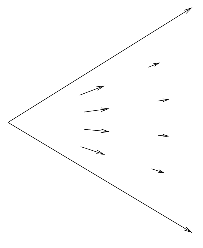
Figure 1: Two examples of drift fields: $cx_{1}^{-1}{\bf e}_{1}$ (left) and $c\|{\bf x}\|^{-1}\hat{\bf x}$ (right).

It is worth comparing the behaviour of the walk in this example in terms of exit from cones to its recurrence/transience behaviour (in terms of returning to bounded sets), which can be obtained from study of the process $\|\xi_{t}\|$. Results of Lamperti [10, 11] (see also [1, 16]) imply that, at least if we assume (A2+),

• If $\beta>1$, $\Xi$ is recurrent in $d=2$ and transient for $d\geq 3$;

• If $\beta<1$, then $\Xi$ is transient for $c>0$ and positive-recurrent for $c<0$.

The case $\beta=1$ is critical from the point of view of the recurrence classification (see in particular the discussion around (4.13) in [10]), and, for any $d$, $\Xi$ can be either positive-recurrent, null-recurrent, or transient, depending on $c$. In particular, there exist $c_{0},c_{1}\in(0,\infty)$ (depending on $d$ and $B_{0}$) such that $\Xi$ is positive-recurrent for $c<-c_{1}<0$ but transient for $c>c_{0}>0$. Thus when $\beta=1$ and $c>c_{0}$, $\Xi$ is transient and so eventually leaves every bounded region, but, on the other hand (by Theorem 2.3(i)) such a walk will also eventually leave any wedge. In other words, although $\|\xi_{t}\|\to\infty$ the walk has no limiting direction.

Example 3: Random walks with drift in the principal direction.

Let $d\geq 2$. It is interesting to contrast two apparently similar types of random walk on the half-space $\mathcal{W}_{d}({\bf e}_{1};\pi/2)$. Suppose that (A1) and (A2+) hold. Suppose either

• for some $c\in\mathbb{R},\beta>0$, for ${\bf x}\in\mathcal{W}_{d}({\bf e}_{1};\pi/2)$, $\mu({\bf x})=c\|{\bf x}\|^{-\beta}{\bf e}_{1}$; or

• for some $c\in\mathbb{R},\beta>0$, for ${\bf x}\in\mathcal{W}_{d}({\bf e}_{1};\pi/2)$, $\mu({\bf x})=cx_{1}^{-\beta}{\bf e}_{1}$.

An example of a suitable drift field in case (b) ($d=2$) is illustrated in the first part of Figure 1. The following result is again a consequence of Theorems 2.1 and 2.2, but requires some extra work: we present its proof at the end of Section 3.

Theorem 2.4

Suppose $\Xi$ is as in Example 3. Suppose $\beta=1$. If $\alpha\in(0,\pi/2)$, then in either case (a) or (b), for any ${\bf x}\in\mathcal{W}_{d}({\bf e}_{1};\alpha)$,

$${\mathbb{P}}[\tau_{\alpha}<\infty\mid\xi_{0}={\bf x}]=1.$$

On the other hand, in case (a), for any ${\bf x}\in\mathcal{W}_{d}({\bf e}_{1};\pi/2)$,

$${\mathbb{P}}[\tau_{\pi/2}<\infty\mid\xi_{0}={\bf x}]=1,$$

but in case (b) there exists $c_{0}\in(0,\infty)$ such that for $c>c_{0}$ and any ${\bf x}\in\mathcal{W}_{d}({\bf e}_{1};\pi/2)$,

$$\|\xi_{t}\|\to\infty,\leavevmode\nobreak\ \leavevmode\nobreak\ \leavevmode\nobreak\ {\rm and}\leavevmode\nobreak\ \leavevmode\nobreak\ \leavevmode\nobreak\ \xi_{t}\cdot{\bf e}_{1}\to\infty\leavevmode\nobreak\ \leavevmode\nobreak\ \leavevmode\nobreak\ {\rm a.s.}.$$

Theorem 2.4 shows that the difference in qualitative behaviour between cases (a) and (b) is manifest in terms of leaving the half-space. In particular, when the mean drift is $c/x_{1}$ in the ${\bf e}_{1}$ direction, the walk leaves a wedge of angle $\alpha<\pi/2$, but, for $c$ large enough, with positive probability eventually remains in the half-plane. However when the mean drift is $c/\|{\bf x}\|$ in the ${\bf e}_{1}$ direction, the walk always leaves the wedge, even when $\alpha=\pi/2$. The instance of Example 3, case (b), when $\alpha=\pi/2$ demonstrates homogeneity in the ${\bf e}_{2}$ direction, and so is related to the one-dimensional so-called Lamperti problem named after [10, 11]. In the case $\alpha=\pi/2$, case (a) demonstrates a more localized perturbation, since near the boundary of the half-plane we can have $\|{\bf x}\|\gg x_{1}$.

The primary interest of Example 3 is the case $\beta=1$. For reasons of space we do not consider here the case $\beta\in(0,1)$ of Example 3 (either (a) or (b)); we expect that this case too can be studied using our methods.

Example 4: Random walk half-plane excursion.

We point out a particularly simple case of Example 3, case (b) above, which is of interest in its own right. This is the so-called random walk half-plane excursion (see [14], pp. 1–2). This process is obtained, loosely speaking, by conditioning a simple symmetric random walk on $\mathbb{Z}^{2}$ never to exit a half-plane: see [14] for details. The construction readily extends to general dimensions $d\geq 2$, but for simplicity we discuss the planar case. In this case $\Xi$ has transition probabilities

$${\mathbb{P}}[\xi_{t+1}=(x_{1},x_{2}\pm 1)\mid\xi_{t}=(x_{1},x_{2})] =\frac{1}{4}$$

$${\mathbb{P}}[\xi_{t+1}=(x_{1}\pm 1,x_{2})\mid\xi_{t}=(x_{1},x_{2})] =\frac{x_{1}\pm 1}{4x_{1}},$$

for $(x_{1},x_{2})\in\mathbb{Z}^{2}$, $x_{1}\geq 1$. Hence

$$\mu({\bf x})=\frac{1}{2x_{1}}{\bf e}_{1},$$

and we are in the case of Example 3(b) as described above. Theorem 2.4 implies that for any $\alpha\in(0,\pi/2)$, the walk leaves the wedge $\mathcal{W}_{2}({\bf e}_{1};\alpha)$ in finite time almost surely. On the other hand, note that $\Xi$ is transient and in fact $\xi_{t}\cdot{\bf e}_{1}\to\infty$ almost surely, by for instance Lamperti’s results [10] (in fact one can take $c_{0}=1/4$ in Theorem 2.4 above, so the final statement of that theorem applies: see the proof of Theorem 2.4 in Section 3).

Example 5: Random walk in random environment.

We give a final example of a slightly different flavour. Let $d\geq 2$. Suppose that each site ${\bf x}\in\mathbb{Z}^{d}$ carries random $d$-vectors ${\bf Y}^{\bf x}$ and $\chi^{\bf x}$, all independent, where ${\bf Y}^{\bf x}=(Y^{\bf x}_{1},\ldots,Y^{\bf x}_{d})$ has an arbitrary distribution (possibly even dependent on ${\bf x}$) on the simplex $\{(y_{1},\ldots,y_{d})\in[0,\infty)^{d}:y_{1}+\cdots+y_{d}=1\}$, and $\chi^{\bf x}=(\chi^{\bf x}_{1},\ldots,\chi^{\bf x}_{d})$ is an independent copy of $\chi=(\chi_{1},\ldots,\chi_{d})$, whose components $|\chi_{i}|$ are bounded uniformly in $i$. Let $\omega:=(({\bf Y}^{\bf x},\chi^{\bf x}))_{{\bf x}\in\mathbb{Z}^{d}}$ be the random environment. Given $\omega$, define a nearest-neighbour Markovian random walk $\Xi$ on $\mathbb{Z}^{d}$ via its transition law ${\mathbb{P}}_{\omega}$ given by, for $i\in\{1,\ldots,d\}$,

$${\mathbb{P}}_{\omega}[\xi_{t+1}-\xi_{t}={\bf e}_{i}\mid\xi_{t}={\bf x}]=\frac{1}{4d}+\frac{Y^{\bf x}_{i}}{4}+\frac{\chi^{\bf x}_{i}}{\|{\bf x}\|},\leavevmode\nobreak\ \leavevmode\nobreak\ \leavevmode\nobreak\ {\mathbb{P}}_{\omega}[\xi_{t+1}-\xi_{t}=-{\bf e}_{i}\mid\xi_{t}={\bf x}]=\frac{1}{4d}+\frac{Y^{\bf x}_{i}}{4}-\frac{\chi^{\bf x}_{i}}{\|{\bf x}\|},$$

unless either of these quantities lies outside the interval $[\frac{1}{4d},1-\frac{1}{4d}]$, in which case we replace both probabilities in question by $\frac{1}{4d}+\frac{Y^{\bf x}_{i}}{4}$ (for almost every $\omega$, this modification will only apply within a finite ball around the origin). Thus $\Xi$ is a random walk in random environment (RWRE). Then, given $\omega$, $\mu({\bf x})=2\|{\bf x}\|^{-1}(\chi^{\bf x}_{1},\ldots,\chi^{\bf x}_{d})$, so that $\|\mu({\bf x})\|=O(\|{\bf x}\|^{-1})$, uniformly for almost every $\omega$, by the conditions on $\chi$. Thus a consequence of Theorem 2.1 is that for almost every $\omega$, for any $\alpha\in(0,\pi)$, $\tau_{\alpha}<\infty$ a.s.. To the best of the authors’ knowledge, the recurrence/transience classification of this RWRE is at present an open problem. An analogous model in $d=1$ where $Y^{\bf x}_{1}\equiv 1$ for all ${\bf x}$ (random perturbation of the simple symmetric random walk on $\mathbb{Z}^{+}$) was studied in [19]: Theorem 2 parts (iii)–(v) in [19] give the complete recurrence classification in that case.

2.4 Extensions, open problems, and further remarks

As we have already indicated, we essentially prove Theorem 2.2 without the assumptions of time-homogeneity or the Markov property (see Section 5 below). It should be possible to prove an appropriate extension of Theorem 2.1 in similar generality. The assumption of the state-space being $\mathbb{Z}^{d}$ is not essentially used in the proof of Theorem 2.2, which we could have stated for more general walks on $\mathbb{R}^{d}$ under an appropriate analogue of (A1); the state-space assumption is central to the decomposition idea in the proof of Theorem 2.1 (see Section 4), but we believe that the method should extend to more general state-spaces assuming an appropriate generalization of the isotropy condition (A1).

As mentioned above, condition (A1) is more general than it might first appear. In fact it is equivalent to the following.

• There exist $\kappa>0$, and $k_{i}\in\mathbb{N}$, $n_{i}\in\mathbb{N}$ for $i\in\{\pm 1,\pm 2,\ldots,\pm d\}$ such that

  $$\min_{{\bf x}\in\SS}\min_{i\in\{\pm 1,\ldots,\pm d\}}{\mathbb{P}}[\xi_{t+n_{i}}-\xi_{t}=k_{i}{\rm sgn}(i){\bf e}_{|i|}\mid\xi_{t}={\bf x}]\geq\kappa\leavevmode\nobreak\ \leavevmode\nobreak\ \leavevmode\nobreak\ (t\in\mathbb{Z}^{+}).$$

Proposition 2.1

Conditions (A1) and (A1^′) are equivalent.

We prove Proposition 2.1 in Section 3. It seems unlikely that the conditions (A1) and (A2) can be relaxed to any significant degree in Theorems 2.1 and 2.2. If (A1) is absent, Theorem 2.1 may fail by the walk getting trapped in a low-dimensional subspace. For example, if the only possible jumps of the walk are in the $\pm{\bf e}_{1}$ directions, it will be trapped on a line. Then one-dimensional results (see e.g. [10]) imply that even for a mean drift of magnitude $O(\|{\bf x}\|^{-1})$ the process can be transient in the positive ${\bf e}_{1}$ direction, and so will with positive probability never leave any cone with principal axis in the ${\bf e}_{1}$ direction, contradiction Theorem 2.1.

In Theorem 2.2, some condition such as (A1) is needed to ensure that $\limsup_{t\to\infty}\|\xi_{t}\|=+\infty$ a.s., or else the walk can get stuck in a finite ball around the origin before the drift asymptotics take effect. We suspect that the moment condition (A2) is close to optimal in Theorem 2.1. It seems likely that in Theorem 2.2, (A2) can be replaced by a uniform bound on $1+\beta+{\varepsilon}<2$ moments $({\varepsilon}>0)$, by a more delicate analysis in Lemma 5.2 below. To avoid additional complications, here we are satisfied with the uniform assumption (A2) throughout.

Several open problems remain. Perhaps the most interesting, and the natural next question to address, is the study of the tails (or moments) of $\tau_{\alpha}$ when $\|\mu({\bf x})\|=O(\|{\bf x}\|^{-1})$. It is not hard to see (for instance by comparison with one-dimensional results such as [11, 1]) that there exists a wide array of possible tail behaviours for $\tau_{\alpha}$. The authors have studied the case $d=2$, under some additional assumptions, in [15]: of course, covariance structure of the increments is crucial here (cf. [9]). In particular, in [15] we show that in $d=2$, when $\|\mu({\bf x})\|=o(\|{\bf x}\|^{-1})$ the tails of $\tau_{\alpha}$ are, to first order, the same as in the Brownian motion case under assumptions on correlations (cf. Spitzer’s theorem [22]). However, the general picture when $\|\mu({\bf x})\|=O(\|{\bf x}\|^{-1})$ is far from complete even in $d=2$.

2.5 Paper outline

The outline of the remainder of the paper is as follows. In Section 3 we collect some preparatory results and prove Proposition 2.1 and Theorem 2.4. Sections 4 and 5 are devoted to the proofs of Theorems 2.1 and 2.2 respectively. The two proofs are essentially independent, so either of these two sections may be read in isolation. In the first part of each of Sections 4 and 5 we give an outline of the main ideas of the proofs before proceeding with the technical details.

3 Preliminaries

In this section we collect some technical results that we need. The first is a martingale-type criterion for proving ${\mathbb{P}}[T=\infty]>0$ for hitting times $T$. The result is based on a well-known idea (see e.g. [6, Theorem 2.2.2] in the countable Markov chain case).

Lemma 3.1

Let $(X_{t})_{t\in\mathbb{Z}^{+}}$ be a stochastic process on $\mathcal{R}$ adapted to a filtration $({\mathcal{F}}_{t})_{t\in\mathbb{Z}^{+}}$. Suppose $g:\mathcal{R}\to[0,\infty)$ and $\mathcal{A}\subset\mathcal{R}$ (possibly infinite) are such that

$${\mathbb{E}}[g(X_{t+1})-g(X_{t})\mid{\mathcal{F}}_{t}]\leq 0\leavevmode\nobreak\ {\rm on}\leavevmode\nobreak\ \{X_{t}\in\mathcal{R}\setminus\mathcal{A}\},$$ (3.1)

for all $t\in\mathbb{Z}^{+}$. Write $g_{0}:=\inf_{x\in\mathcal{A}}g(x)$. Then for $x_{0}\in\mathcal{R}\setminus\mathcal{A}$, on $\{X_{0}=x_{0}\}$

$${\mathbb{P}}[\min\{t\in\mathbb{Z}^{+}:X_{t}\in\mathcal{A}\}=\infty\mid{\mathcal{F}}_{0}]\geq 1-\frac{g(x_{0})}{g_{0}}.$$

Proof. Let $T=\min\{t\in\mathbb{Z}^{+}:X_{t}\in\mathcal{A}\}$, an $({\mathcal{F}}_{t})_{t\in\mathbb{Z}^{+}}$-stopping time; we need to show ${\mathbb{P}}[T=\infty]>0$. By (3.1), we have that $g(X_{t\wedge T})$ is a supermartingale adapted to $({\mathcal{F}}_{t})_{t\in\mathbb{Z}^{+}}$. Moreover, $g$ is nonnegative so $g(X_{t\wedge T})$ converges a.s. to some limit, say $L$. Then if $X_{0}=x_{0}$ we have

$$g(x_{0})\geq{\mathbb{E}}[L]\geq{\mathbb{E}}[L{\bf 1}_{\{T<\infty\}}]\geq g_{0}{\mathbb{P}}[T<\infty],$$

which implies that ${\mathbb{P}}[T<\infty]\leq g(x_{0})/g_{0}$, as required. $\Box$

The following maximal inequality is Lemma 3.1 in [18].

Lemma 3.2

Let $(Y_{t})_{t\in\mathbb{Z}^{+}}$ be a stochastic process on $[0,\infty)$ adapted to a filtration $({\mathcal{F}}_{t})_{t\in\mathbb{Z}^{+}}$. Suppose that $Y_{0}=y_{0}$ and for some $b\in(0,\infty)$ and all $t\in\mathbb{Z}^{+}$

$${\mathbb{E}}[Y_{t+1}-Y_{t}\mid{\mathcal{F}}_{t}]\leq b\leavevmode\nobreak\ {\rm a.s.}.$$

Then for any $x>0$ and any $t\in\mathbb{N}$

$${\mathbb{P}}\left[\max_{0\leq s\leq t}Y_{s}\geq x\right]\leq(bt+y_{0})x^{-1}.$$

Next we prove Proposition 2.1. The proof is elementary and we do not give all the formal details.

Proof of Proposition 2.1. Clearly (A1) implies (A1^′). So suppose that (A1^′) holds. The following four-step argument shows that (A1) follows.

(i) First we show that without loss of generality we may take $n_{-i}=n_{i}$ for each $i$. This is straightforward, since with positive probability the walk sequentially takes $n_{-i}$ ‘jumps’ of size $k_{i}$ in the ${\bf e}_{i}$ direction and also with positive probability the walk sequentially takes $n_{i}$ ‘jumps’ of size $k_{-i}$ in the $-{\bf e}_{i}$ direction. In either case, the walk has moved a positive distance in time $n_{i}n_{-i}$.

(ii) Next we show that we may take $k_{i}=k_{-i}$ for each $i$. Fix $i$. In view of part (i), we may take $n_{i}=n_{-i}=n$, say. Let

$$s_{i}:=(k_{i}+k_{-i})\max\{k_{i},k_{-i}\}.$$

Without loss of generality, we may suppose $k_{-i}\geq k_{i}$. Then each of the following two events has positive probability: (a) the walk can perform $(k_{i}+k_{-i})k_{-i}$ successive ‘jumps’ of size $k_{i}$ in the ${\bf e}_{i}$ direction; (b) the walk can perform $(k_{i}+k_{-i})k_{i}$ successive ‘jumps’ of size $k_{-i}$ in the $-{\bf e}_{i}$ direction followed by $(k_{i}+k_{-i})(k_{-i}-k_{i})$ successive ‘jumps’ of size $k_{i}$ in the ${\bf e}_{i}$ direction. In either case (a) or (b), the walk ends up at distance $(k_{i}+k_{-i})k_{i}k_{-i}$ from its starting point after time $n(k_{i}+k_{-i})k_{-i}$.

(iii) Next we show that we can take $n_{i}=n_{-i}=n$ for all $i$. Given parts (i) and (ii), we may take $k_{i}=k_{-i}$ and $n_{i}=n_{-i}$ for each $i$. Set $n:=\prod_{i}n_{i}$. For any $i$, the walk has positive probability of performing in succession $n/n_{i}$ ‘jumps’ of size $k_{i}$ in either of the $\pm{\bf e}_{i}$ directions. Such an event takes a total time $n$ and leads to a positive displacement, equal in opposite directions.

(iv) Finally we show that we may take $k_{i}=k_{-i}=k$ for all $i$. Given parts (i)–(iii) we can take $k_{i}=k_{-i}$ and $n_{i}=n$ for all $i$. Set $r:=\prod_{i}k_{i}$. Then for any $i$, with positive probability the walk can perform $2r/k_{i}$ ‘jumps’ of size $k_{i}$ in the direction $\pm{\bf e}_{i}$, taking time $2nr/k_{i}$. Then in time $2n(r/k_{i})(k_{i}-1)$ (an even multiple of $n$) the walk can go back and forth to achieve an additional net displacement of $0$. The walk is then at distance $2r$ from its starting point after a total time $2nr$. Thus (A1) holds with $n_{0}=2nr$ and $k=2r$. This completes the proof. $\Box$

Finally for this section, we give the proof of Theorem 2.4.

Proof of Theorem 2.4. Suppose $\beta=1$. Suppose we are in case (a), so that $\mu({\bf x})=c\|{\bf x}\|^{-1}{\bf e}_{1}$. Then Theorem 2.1 applies and ${\mathbb{P}}[\tau_{\alpha}<\infty]=1$ for any $\alpha\leq\pi/2$. Now suppose we are in case (b), so that $\mu({\bf x})=cx_{1}^{-1}{\bf e}_{1}$. In this case we have for any $\alpha\in(0,\pi/2)$

$$0<\cos\alpha\leq\inf_{{\bf x}\in\mathcal{W}_{d}({\bf e}_{1};\alpha)}\frac{x_{1}}{\|{\bf x}\|}\leq\sup_{{\bf x}\in\mathcal{W}_{d}({\bf e}_{1};\alpha)}\frac{x_{1}}{\|{\bf x}\|}\leq 1,$$

so that (2.1) holds throughout $\mathcal{W}_{d}({\bf e}_{1};\alpha)$. It follows from Theorem 2.1 that ${\mathbb{P}}[\tau_{\alpha}<\infty]=1$ for $\alpha<\pi/2$. Finally consider $\tau_{\pi/2}$. Let $X_{t}=\xi_{t}\cdot{\bf e}_{1}$; then $\tau_{\pi/2}=\min\{t\in\mathbb{Z}^{+}:X_{t}\leq 0\}$. From our conditions on $\Xi$ in this case we have

$${\mathbb{E}}[X_{t+1}-X_{t}\mid\xi_{t}=(x_{1},x_{2})]=cx_{1}^{-1},\leavevmode\nobreak\ \leavevmode\nobreak\ \leavevmode\nobreak\ \sup_{{\bf x}\in\mathcal{W}_{d}({\bf e}_{1};\pi/2)}{\mathbb{E}}[(X_{t+1}-X_{t})^{2+{\varepsilon}}\mid\xi_{t}={\bf x}]<\infty.$$

Thus we can apply results of Lamperti [10, Theorem 3.2] to $X_{t}$ to conclude that ${\mathbb{P}}[\tau_{\pi/2}=\infty]>0$ for $c>c_{0}$ where

$$c_{0}=\frac{1}{2}\sup_{{\bf x}\in\mathcal{W}_{d}({\bf e}_{1};\pi/2)}{\mathbb{E}}[(X_{t+1}-X_{t})^{2}\mid\xi_{t}={\bf x}]\in(0,\infty).$$

This completes the proof. $\Box$

4 Finite exit times: proof of Theorem 2.1

4.1 Outline of the proof

We show in this section that Theorem 2.1 holds: under the conditions of the theorem, with probability $1$ the random walk $\Xi$ will leave any cone $\mathcal{W}_{d}({\bf u};\alpha)$, $\alpha\in(0,\pi)$ after a finite time. There are several steps to the proof but the overall scheme is based on some intuitive ideas, which we now sketch.

The basic element to the proof of Theorem 2.1 is Lemma 4.8, which says that, roughly speaking, starting in any small cone there is positive probability, uniform in the current position of the walk, that the walk hits a neighbouring small cone. To prove this result we need to study hitting-time properties of the walk. Specifically, we need to show that there is a good probability that the walk hits a reasonably-sized set at distance of the order of $\|{\bf x}\|$ starting from ${\bf x}$. The conditions (A1), (A2), and (2.1) are of course crucial here.

In view of (A1) it is natural to work with the ‘$n_{0}$-skeleton’ process $(\xi_{tn_{0}})_{t\in\mathbb{Z}^{+}}$, which we denote $\Xi^{*}$. In Section 4.2 we define a decomposition of the walk $\Xi^{*}$ based on the regularity condition (A1). The basic idea is that since, by (A1), every jump of the walk $\Xi^{*}$ has positive probability of being one of $\pm k{\bf e}_{i}$, we can extract a symmetric random walk from $\Xi^{*}$, leaving a residual process that retains some of the regularity of the original walk, despite no longer being Markovian.

Next, in Section 4.3, we prove our basic hitting-time estimates. The idea now is to treat the two parts of the decomposition separately. The symmetric process is more straightforward to study, and is the part of the walk that will ensure that there is good probability of the walk hitting a particular set some distance away without returning too close to the origin. The technical estimate here is Lemma 4.4.

The next step is to show that the residual process, which has inherited appropriate drift conditions from $\Xi$, will with good probability not travel too far in the same time, so that the walk as a whole has good probability of hitting the desired set. There are complications introduced here as the residual process depends on the realization of the symmetric process; thus we condition on that in our estimates. Under suitable behaviour of both processes, the walk stays far enough from the origin that the drift remains controlled. The technical estimate here is Lemma 4.5.

Based on the estimates for the two parts of our decomposition, we show (in Lemma 4.7) that $\Xi$ hits a suitable set with positive probability. In Section 4.4 we translate this result into our exit-from-cones result, Lemma 4.8, which we use to complete the proof of Theorem 2.1. Our three conditions (A1), (A2), and (2.1) all appear very naturally in this scheme. Having outlined the idea, we now proceed with the technical work.

4.2 Decomposition

In view of condition (A1), it is convenient to consider the random walk at time spacing $n_{0}$, i.e. the embedded (‘skeleton’) process $(\xi_{tn_{0}})_{t\in\mathbb{Z}^{+}}$. For notational convenience, set

$$\xi^{*}_{t}:=\xi_{tn_{0}},\leavevmode\nobreak\ \leavevmode\nobreak\ \leavevmode\nobreak\ (t\in\mathbb{Z}^{+}).$$

Then $\Xi^{*}=(\xi^{*}_{t})_{t\in\mathbb{Z}^{+}}$ is a Markovian random walk on $\SS\subseteq\mathbb{Z}^{d}$ with transition probabilities

$${\mathbb{P}}[\xi^{*}_{t+1}={\bf y}\mid\xi^{*}_{t}={\bf x}]={\mathbb{P}}[\xi_{n_{0}}={\bf y}\mid\xi_{0}={\bf x}],$$

and $\xi^{*}_{0}=\xi_{0}$. The walk $\Xi^{*}$ inherits regularity from $\Xi$, as the next result shows.

Lemma 4.1

(i) If (A1) holds then

$$\min_{{\bf x}\in\SS}\min_{i\in\{1,\ldots,d\}}{\mathbb{E}}[|(\xi^{*}_{t+1}-\xi^{*}_{t})\cdot{\bf e}_{i}|^{2}\mid\xi^{*}_{t}={\bf x}]\geq 2\kappa k^{2}>0.$$ (4.1)

(ii) If (A2) holds then

$$\max_{{\bf x}\in\SS}{\mathbb{E}}[\|\xi^{*}_{t+1}-\xi^{*}_{t}\|^{2}\mid\xi^{*}_{t}={\bf x}]\leq n_{0}^{2}B_{0}<\infty.$$ (4.2)

(iii) If (A2) and (2.1) hold, then

$$\|{\mathbb{E}}[\xi^{*}_{t+1}-\xi^{*}_{t}\mid\xi^{*}_{t}={\bf x}]\|=O(\|{\bf x}\|^{-1}).$$ (4.3)

Proof. By time-homogeneity, it suffices to simplify notation by taking $t=0$ throughout. Part (i) is immediate from (A1). For part (ii), we have by the triangle inequality that ${\mathbb{E}}[\|\xi^{*}_{1}-\xi^{*}_{0}\|^{2}\mid\xi^{*}_{0}={\bf x}]$ is equal to

$${\mathbb{E}}\left[\left\|\sum_{j=1}^{n_{0}}(\xi_{j}-\xi_{j-1})\right\|^{2}\mid\xi_{0}={\bf x}\right]\leq{\mathbb{E}}\left[\left(\sum_{j=1}^{n_{0}}\|\xi_{j}-\xi_{j-1}\|\right)^{2}\mid\xi_{0}={\bf x}\right]$$

$$\leavevmode\nobreak\ \leavevmode\nobreak\ =\sum_{j=1}^{n_{0}}\sum_{k=1}^{n_{0}}{\mathbb{E}}\left[\|\xi_{j}-\xi_{j-1}\|\|\xi_{k}-\xi_{k-1}\|\mid\xi_{0}={\bf x}\right]\leq\left(\sum_{j=1}^{n_{0}}({\mathbb{E}}[\|\xi_{j}-\xi_{j-1}\|^{2}\mid\xi_{0}={\bf x}])^{1/2}\right)^{2},$$

by the Cauchy–Schwarz inequality. Here for $j\geq 1$, by the Markov property,

$${\mathbb{E}}[\|\xi_{j}-\xi_{j-1}\|^{2}\mid\xi_{0}={\bf x}]=\sum_{{\bf y}\in\SS}{\mathbb{E}}[\|\xi_{j}-\xi_{j-1}\|^{2}\mid\xi_{j-1}={\bf y}]{\mathbb{P}}[\xi_{j-1}={\bf y}\mid\xi_{0}={\bf x}]\leq B_{0},$$

by (A2). Thus we obtain (4.2). Finally we prove part (iii). First we show that the event

$$E({\bf x}):=\left\{\max_{0\leq s\leq n_{0}}\|\xi_{s}-{\bf x}\|>\frac{1}{2}\|{\bf x}\|\right\}$$

has small probability given $\xi_{0}={\bf x}$. For ${\bf x}\in\mathbb{R}^{d}$ and $t\in\mathbb{Z}^{+}$, set $W^{\bf x}_{s}:=\|\xi_{s}-{\bf x}\|^{2}$. We have

$${\mathbb{E}}[W^{\bf x}_{s+1}-W^{\bf x}_{s}\mid\xi_{s}={\bf y}] ={\mathbb{E}}[\|\xi_{s+1}-\xi_{s}\|^{2}+2({\bf y}-{\bf x})\cdot(\xi_{s+1}-\xi_{s})\mid\xi_{s}={\bf y}]$$

$$\leq B_{0}+2\|{\bf y}-{\bf x}\|\|\mu({\bf y})\|,$$

using (A2). Now using (2.1) we see that there exists $C\in(0,\infty)$ such that

$${\mathbb{E}}[W^{\bf x}_{s+1}-W^{\bf x}_{s}\mid\xi_{s}={\bf y}]\leq C(1+\|{\bf x}\|^{-1}\|{\bf y}\|).$$ (4.4)

Now define $T({\bf x}):=\min\{s\in\mathbb{Z}^{+}:W_{s}^{\bf x}>\|{\bf x}\|^{2}/4\}$. Note that for $s<T({\bf x})$, $\|{\bf x}\|/2\leq\|\xi_{s}\|\leq 3\|{\bf x}\|/2$. Then given $\xi_{0}={\bf x}$, on $\{s<T({\bf x})\}$ we have from (4.4) that ${\mathbb{E}}[W^{\bf x}_{s+1}-W^{\bf x}_{s}\mid\xi_{s}]\leq 5C/2<\infty$. Hence we can apply Lemma 3.2 to $W^{\bf x}_{s\wedge T({\bf x})}$ to obtain

$${\mathbb{P}}\left[\max_{0\leq s\leq n_{0}}W_{s\wedge T({\bf x})}^{\bf x}>\frac{1}{4}\|{\bf x}\|^{2}\mid\xi_{0}={\bf x}\right]\leq C\|{\bf x}\|^{-2},$$

for some $C\in(0,\infty)$. However $T({\bf x})\leq n_{0}$ implies that

$$\max_{0\leq s\leq n_{0}}W_{s\wedge T({\bf x})}^{\bf x}\geq W_{T({\bf x})}^{\bf x}>\frac{1}{4}\|{\bf x}\|^{2},$$

by definition of $T({\bf x})$. Hence

$${\mathbb{P}}[E({\bf x})\mid\xi_{0}={\bf x}]={\mathbb{P}}[T({\bf x})\leq n_{0}\mid\xi_{0}={\bf x}]\leq C\|{\bf x}\|^{-2}.$$ (4.5)

Now by partitioning on $E({\bf x})$ and applying the triangle inequality,

$$\|{\mathbb{E}}[\xi^{*}_{1}-\xi^{*}_{0}\mid\xi^{*}_{0}={\bf x}]\| \leq\sum_{s=1}^{n_{0}}\|{\mathbb{E}}[\xi_{s}-\xi_{s-1}\mid E^{c}({\bf x}),\xi_{0}={\bf x}]\|$$

$$\leavevmode\nobreak\ \leavevmode\nobreak\ +\sum_{s=1}^{n_{0}}\|{\mathbb{E}}[(\xi_{s}-\xi_{s-1}){\bf 1}_{E({\bf x})}\mid\xi_{0}={\bf x}]\|,$$ (4.6)

where $E^{c}({\bf x})$ is the complementary event to $E({\bf x})$. Now using the elementary inequality that for ${\bf X}$ a random $d$-vector $\|{\mathbb{E}}[{\bf X}]\|\leq d{\mathbb{E}}\|{\bf X}\|$, we have that

$$\|{\mathbb{E}}[(\xi_{s}-\xi_{s-1}){\bf 1}_{E({\bf x})}\mid\xi_{0}={\bf x}]\|\leq d{\mathbb{E}}[\|\xi_{s}-\xi_{s-1}\|{\bf 1}_{E({\bf x})}\mid\xi_{0}={\bf x}],$$

so that by Cauchy–Schwarz, (A2), and (4.5),

$$\|{\mathbb{E}}[(\xi_{s}-\xi_{s-1}){\bf 1}_{E({\bf x})}\mid\xi_{0}={\bf x}]\|$$

$$\leavevmode\nobreak\ \leavevmode\nobreak\ \leq d({\mathbb{E}}[\|\xi_{s}-\xi_{s-1}\|^{2}\mid\xi_{0}={\bf x}])^{1/2}({\mathbb{P}}[E({\bf x})\mid\xi_{0}={\bf x}])^{1/2}\leq C\|{\bf x}\|^{-1},$$

for some $C\in(0,\infty)$. On the other hand, on $E^{c}({\bf x})\cap\{\xi_{0}={\bf x}\}$ we have from (2.1) that

$$\max_{0\leq s\leq n_{0}}\|{\mathbb{E}}[\xi_{s}-\xi_{s-1}\mid E^{c}({\bf x}),\xi_{0}={\bf x}]\|\leq\max_{{\bf y}\in\SS:(1/2)\|{\bf x}\|\leq\|{\bf y}\|\leq(3/2)\|{\bf x}\|}\|\mu({\bf y})\|^{-1},$$

which is again $O(\|{\bf x}\|^{-1})$. Combining the two estimates for the terms on the right-hand side of (4.2) we obtain (4.3). $\Box$

The next result establishes the decomposition. Specifically, we decompose the jump of $\Xi^{*}$ at time $t$ into a symmetric component ($V_{t+1}$), and a residual component ($\zeta_{t+1}$), such that at any time $t$ only one of the two components is present in a particular realization.

Lemma 4.2

Suppose (A1) holds. There exist sequences of random variables $(V_{t})_{t\in\mathbb{N}}$ and $(\zeta_{t})_{t\in\mathbb{N}}$ such that:

• the $(V_{t})_{t\in\mathbb{N}}$ are i.i.d. with $V_{1}\in\{{\bf 0},\pm k{\bf e}_{1},\ldots,\pm k{\bf e}_{d}\}$ and

  $${\mathbb{P}}[V_{1}={\bf 0}]=1-2d\kappa,\leavevmode\nobreak\ \leavevmode\nobreak\ \leavevmode\nobreak\ {\mathbb{P}}[V_{1}=-k{\bf e}_{i}]={\mathbb{P}}[V_{1}=+k{\bf e}_{i}]=\kappa;$$

• $\zeta_{t+1}\in\mathbb{Z}^{d}$ with ${\mathbb{P}}[\zeta_{t+1}={\bf 0}\mid V_{t}\neq{\bf 0}]=1$ and

  $$\zeta_{t+1}=\left(\xi^{*}_{t+1}-\xi^{*}_{t}-V_{t+1}\right){\bf 1}_{\{V_{t+1}={\bf 0}\}}=(\xi^{*}_{t+1}-\xi^{*}_{t}){\bf 1}_{\{V_{t+1}={\bf 0}\}};$$ (4.7)

• we can decompose the jumps of $\Xi^{*}$ via

  $$\xi^{*}_{t+1}-\xi^{*}_{t}=V_{t+1}+\zeta_{t+1}=V_{t+1}{\bf 1}_{\{V_{t+1}\neq{\bf 0}\}}+\zeta_{t+1}{\bf 1}_{\{V_{t+1}={\bf 0}\}}\leavevmode\nobreak\ \leavevmode\nobreak\ \leavevmode\nobreak\ (t\in\mathbb{Z}^{+}).$$ (4.8)

Proof. The statement of the lemma follows directly from (A1), but for clarity let us give an explicit construction of the variables $V_{t}$ and $\zeta_{t}$. By the time-homogeneity and Markov assumptions on $\Xi$ (hence $\Xi^{*}$) for each ${\bf x}\in\mathbb{Z}^{d}$ there exists a sequence of i.i.d. random vectors $\Delta^{\bf x}_{1},\Delta^{\bf x}_{2},\ldots$, independent for each ${\bf x}$, such that we can realize $\xi^{*}_{t+1}-\xi^{*}_{t}$ as

$$\xi^{*}_{t+1}-\xi^{*}_{t}=\sum_{{\bf x}\in\SS}\Delta^{\bf x}_{t+1}{\bf 1}_{\{\xi^{*}_{t}={\bf x}\}}.$$ (4.9)

Condition (A1) implies that

$$\min_{{\bf x}\in\SS}{\mathbb{P}}[\Delta^{\bf x}_{t+1}=k{\bf e}_{i}]\geq\kappa,$$

and similarly for $-k{\bf e}_{i}$. It follows that we can write $\Delta^{\bf x}_{t+1}=V_{t+1}+\zeta^{\bf x}_{t+1}$ where $V_{t+1}$ is as described in part (i) of the lemma. Then (4.9) becomes

$$\xi^{*}_{t+1}-\xi^{*}_{t}=V_{t+1}+\sum_{{\bf x}\in\SS}\zeta^{\bf x}_{t+1}{\bf 1}_{\{\xi^{*}_{t}={\bf x}\}};$$

this final sum we denote by $\zeta_{t+1}$, and parts (ii) and (iii) of the lemma follow. $\Box$

For $t\in\mathbb{N}$, (4.8) yields a decomposition for $\xi^{*}_{t}$ as

$$\xi^{*}_{t}-\xi_{0}=\sum_{s=1}^{t}(V_{s}+\zeta_{s}).$$ (4.10)

Note that the residual increments $\zeta_{1},\zeta_{2},\ldots$ have a rather complicated structure (and are certainly not independent); however, they do inherit regularity properties from $\Xi$, as we summarize in the next lemma.

Lemma 4.3

Suppose (A1) and (A2) hold, and $\zeta_{t+1}$ is as in Lemma 4.2. Then

$$\max_{{\bf x}\in\SS}{\mathbb{E}}[\|\zeta_{t+1}\|^{2}\mid\xi^{*}_{t}={\bf x}] \leq n_{0}^{2}B_{0}<\infty$$ (4.11)

$$\|{\mathbb{E}}[\zeta_{t+1}\mid\xi^{*}_{t}={\bf x}]\| =\|{\mathbb{E}}[\xi^{*}_{t+1}-\xi^{*}_{t}\mid\xi^{*}_{t}={\bf x}]\|.$$ (4.12)

Proof. From (4.7) we have $\|\zeta_{t+1}\|\leq\|\xi^{*}_{t+1}-\xi^{*}_{t}\|$ a.s., while conditioning on $\xi^{*}_{t}={\bf x}$, taking expectations on both sides of the first equality in (4.8) and noting that ${\mathbb{E}}[V_{t+1}\mid\xi_{t}^{*}={\bf x}]={\bf 0}$, we have

$${\mathbb{E}}[\zeta_{t+1}\mid\xi^{*}_{t}={\bf x}]={\mathbb{E}}[\xi^{*}_{t+1}-\xi^{*}_{t}\mid\xi^{*}_{t}={\bf x}].$$

These two facts combined with Lemma 4.1 yield the stated results. $\Box$

4.3 Hitting-time estimates

Having established our decomposition, we will eventually use it to show that under the conditions of Theorem 2.1, $\Xi$ will exit any cone in any particular direction with good probability: see Section 4.4 below. In order to establish this result, the main ingredient will be the somewhat more specific Lemma 4.7 below, which says that, under appropriate conditions, $\Xi$ hits some suitable ball with positive probability. In order to prove Lemma 4.7, we need to work separately on the two parts of the decomposition. We deal with the residual process in Lemma 4.5. First we study the symmetric process, building up to Lemma 4.4.

Set $Y_{0}:={\bf 0}$ and for $t\in\mathbb{N}$

$$Y_{t}:=Y_{0}+\sum_{s=1}^{t}V_{s}.$$ (4.13)

The process $(Y_{t})_{t\in\mathbb{Z}^{+}}$ is a symmetric, homogeneous random walk on $\mathbb{Z}^{d}$ with ${\mathbb{P}}[Y_{t}=Y_{t-1}]={\mathbb{P}}[V_{t}={\bf 0}]=1-2d\kappa<1$ and jumps of size $k$. For $r>0$, ${\bf y}\in\mathbb{R}^{d}$ write $B_{r}({\bf y})$ for the Euclidean $d$-ball $B_{r}({\bf y}):=\{{\bf x}\in\mathbb{R}^{d}:\|{\bf x}-{\bf y}\|<r\}$; set $B_{r}:=B_{r}({\bf 0})$. Let $\Lambda\subset\mathbb{R}^{d}$ be a convex set and $r>0$. Define stopping times

$$\sigma(\Lambda):=\min\{t\in\mathbb{Z}^{+}:Y_{t}\in\Lambda\},\leavevmode\nobreak\ \leavevmode\nobreak\ \leavevmode\nobreak\ \rho(r):=\min\{t\in\mathbb{Z}^{+}:\|Y_{t}\|\geq r\}.$$ (4.14)

Our first result is to show that with positive probability (uniformly in $N$) in time ${\varepsilon}N^{2}$, for small enough ${\varepsilon}$, the symmetric walk $Y_{t}$ hits a subset of $B_{N}$ of volume $\lambda N^{d}$ before $B_{h_{0}N}$, where $\lambda>0$ is fixed and $h_{0}$ depends only on the parameters in condition (A1).

Lemma 4.4

Let $d\geq 2$. Let $N\geq 1$. Let $\Lambda_{N}\subseteq B_{N}$ be a convex set with $d$-dimensional volume at least $\lambda N^{d}$ for some $\lambda>0$. Then with $\sigma$ and $\rho$ as defined at (4.14), there exist constants (not depending on $N$) $N_{1}\geq 1$, $h_{0}\in[2^{-1/2},\infty)$, and ${\varepsilon}_{1}\in(0,1)$ such that for all $N\geq N_{0}$, any $h\geq h_{0}$, and any ${\varepsilon}\in(0,{\varepsilon}_{1})$

$${\mathbb{P}}[\sigma(\Lambda_{N})\leq\lfloor{\varepsilon}N^{2}\rfloor\wedge\rho(hN)]\geq\delta$$

for some $\delta>0$ depending only on ${\varepsilon}$, $k$, $\kappa$, $\lambda$ and $d$, but not on $N$.

Proof. Let ${\varepsilon}>0$. Note that ${\mathbb{P}}[\sigma(\Lambda_{N})\leq\lfloor{\varepsilon}N^{2}\rfloor]\geq{\mathbb{P}}[Y_{\lfloor{\varepsilon}N^{2}\rfloor}\in\Lambda_{N}]$. By the standard multivariate central limit theorem for sums of i.i.d. random vectors, and the fact that ${\mathbb{E}}[(V_{1}\cdot{\bf e}_{1})^{2}]=2k^{2}\kappa$ by Lemma 4.2(i), we have that for measurable $A\subset\mathbb{R}^{d}$

$${\mathbb{P}}[(2k^{2}\kappa t)^{-1/2}Y_{t}\in A]\to(2\pi)^{-d/2}\int_{A}\exp\{-\|{\bf x}\|^{2}/2\}\mathrm{d}{\bf x},$$

as $t\to\infty$. Taking $A=(2k^{2}\kappa t)^{-1/2}\Lambda_{N}$ and $t=\lfloor{\varepsilon}N^{2}\rfloor$, we have that the volume of $A$ is at least $(2k^{2}\kappa{\varepsilon})^{-1/2}\lambda$, so that for some $N_{1}\geq 1$ and all $N\geq N_{1}$

$${\mathbb{P}}[Y_{\lfloor{\varepsilon}N^{2}\rfloor}\in\Lambda_{N}]\geq\frac{1}{2}(2\pi)^{-d/2}(2k^{2}\kappa{\varepsilon})^{-1/2}\lambda\exp\left\{-\frac{1}{2}(2k^{2}\kappa{\varepsilon}N^{2})^{-1}\sup_{{\bf x}\in\Lambda_{N}}\|{\bf x}\|^{2}\right\}$$

$$\geq\frac{1}{2}(2\pi)^{-d/2}(2k^{2}\kappa{\varepsilon})^{-1/2}\lambda\exp\left\{-\frac{1}{4k^{2}\kappa{\varepsilon}}\right\},$$ (4.15)

since $\Lambda_{N}\subseteq B_{N}$. On the other hand, we claim that for any $r>0$ and $t\in\mathbb{N}$,

$${\mathbb{P}}[\rho(r)\leq t]={\mathbb{P}}\left[\max_{0\leq s\leq t}\|Y_{s}\|\geq r\right]\leq 4d\exp\left\{-\frac{r^{2}}{2dk^{2}t}\right\}.$$ (4.16)

To obtain the inequality in (4.16), note that

$${\mathbb{P}}\left[\max_{0\leq s\leq t}\|Y_{s}\|\geq r\right]\leq d{\mathbb{P}}\left[\max_{0\leq s\leq t}|Y_{s}\cdot{\bf e}_{1}|\geq d^{-1/2}r\right],$$

and then combine inequalities of Lévy (see e.g. [7, p. 139]) and Hoeffding (see e.g. [7, p. 120]) on sums of i.i.d. mean-zero bounded random variables to obtain

$${\mathbb{P}}\left[\max_{0\leq s\leq t}|Y_{s}\cdot{\bf e}_{1}|\geq d^{-1/2}r\right]\leq 2{\mathbb{P}}\left[|Y_{t}\cdot{\bf e}_{1}|\geq d^{-1/2}r\right]\leq 4\exp\left\{-\frac{r^{2}}{2dk^{2}t}\right\}.$$

Hence combining (4.3) and the $r=hN$, $t=\lfloor{\varepsilon}N^{2}\rfloor$ case of (4.16)

$${\mathbb{P}}[\{\rho(hN)\leq\lfloor{\varepsilon}N^{2}\rfloor\}\cup\{\sigma(\Lambda_{N})>\lfloor{\varepsilon}N^{2}\rfloor\}]$$

$$\leavevmode\nobreak\ \leavevmode\nobreak\ \leq 1-\frac{1}{2}(2\pi)^{-d/2}(2k^{2}\kappa{\varepsilon})^{-1/2}\lambda\exp\left\{-\frac{1}{4k^{2}\kappa{\varepsilon}}\right\}+4d\exp\left\{-\frac{h^{2}}{2dk^{2}{\varepsilon}}\right\}\leq 1-\delta,$$

for some $\delta>0$, not depending on $N$, if we choose $h\geq h_{0}:=(d/\kappa)^{1/2}\geq 2^{-1/2}$ and ${\varepsilon}>0$ small enough. The statement of the lemma follows. $\Box$

Let $Z_{0}:={\bf 0}$ and for $t\in\mathbb{N}$ let

$$Z_{t}:=Z_{0}+\sum_{s=1}^{t}\zeta_{s}.$$ (4.17)

Thus $(Z_{t})_{t\in\mathbb{Z}^{+}}$ is the residual part of the process $(\xi^{*}_{t})_{t\in\mathbb{Z}^{+}}$ after the symmetric process $(Y_{t})_{t\in\mathbb{Z}^{+}}$ has been extracted. Indeed, with $Y_{t},Z_{t}$ as defined at (4.13), (4.17) we have from (4.10) that for $t\in\mathbb{N}$

$$\xi^{*}_{t}-\xi_{0}=Y_{t}+Z_{t}.$$ (4.18)

We next show that with good probability the residual process $(Z_{t})_{t\in\mathbb{Z}^{+}}$ does not exit from a suitable ball around ${\bf 0}$ by time $\lfloor{\varepsilon}N^{2}\rfloor$. By construction the process $(Z_{t})_{t\in\mathbb{Z}^{+}}$ depends upon $(V_{t})_{t\in\mathbb{N}}$ because the distribution of $\zeta_{t+1}$ depends upon the value of $\xi^{*}_{t}$. For $t\in\mathbb{N}$, let $\Omega_{V}(t):=\{{\bf 0},\pm k{\bf e}_{i},\ldots,\pm k{\bf e}_{d}\}^{t}$ and let $\omega_{V}\in\Omega_{V}(t)$ denote a generic realization of the sequence $(V_{1},\ldots,V_{t})$. For $r>0$ define

$$\Omega_{V,r}(t)=\{\omega_{V}\in\Omega_{V}(t):t<\rho(r)(\omega_{V})\},$$

i.e., the set of those paths $\omega_{V}$ for which $\|Y_{s}\|<r$ for all $s\leq t$. Our next result, Lemma 4.5, gives control over the deviations of $Z_{t}$. The choice of $3/4$ as the lower bound in Lemma 4.5 is fairly arbitrary: any lower bound in $(0,1)$ can be obtained for ${\varepsilon}$ small enough, but $3/4$ is good enough for us.

Lemma 4.5

Let $h\in(0,\infty)$. Suppose (A1) and (A2) hold and that for some $K_{0}\in(0,\infty)$

$$\max_{{\bf x}\in\SS\cap B_{(1+h)N}(\xi_{0})}\|{\mathbb{E}}[\xi^{*}_{t+1}-\xi^{*}_{t}\mid\xi^{*}_{t}={\bf x}\|\leq K_{0}N^{-1},$$ (4.19)

for all $N\geq 1$. Let $c\in(0,1/2]$. There exists ${\varepsilon}_{2}>0$ not depending on $N$ (but depending on $c$ and $K_{0}$) such that for all ${\varepsilon}\in(0,{\varepsilon}_{2})$, all $N\geq 1$, and all $\omega_{V}\in\Omega_{V,hN}(\lfloor{\varepsilon}N^{2}\rfloor)$

$${\mathbb{P}}\left[\max_{0\leq t\leq\lfloor{\varepsilon}N^{2}\rfloor}\|Z_{t}\|\leq cN\mid(V_{1},\ldots,V_{\lfloor{\varepsilon}N^{2}\rfloor})=\omega_{V},Z_{0}={\bf 0}\right]\geq\frac{3}{4}.$$

Proof. Let $c\in(0,1/2]$. For the duration of this proof, define the stopping time

$$\tau_{0}:=\min\{t\in\mathbb{Z}^{+}:\|Z_{t}\|>cN\}.$$

For the duration of this proof, let ${\mathcal{G}}_{t}=\sigma(\xi^{*}_{0},\xi^{*}_{1},\ldots,\xi^{*}_{t},V_{1},\ldots,V_{t})$. Then $\zeta_{1},\ldots,\zeta_{t}$ and $Z_{0},Z_{1},\ldots,Z_{t}$ are ${\mathcal{G}}_{t}$-measurable, and $\tau_{0}$ is a $({\mathcal{G}}_{t})_{t\in\mathbb{Z}^{+}}$ stopping time. Consider the stopped square-deviation process defined for $t\in\mathbb{Z}^{+}$ by $W_{t}:=\|Z_{t\wedge\tau_{0}}\|^{2}$; $W_{t}$ is then ${\mathcal{G}}_{t}$-adapted. Suppose that $t\leq\lfloor{\varepsilon}N^{2}\rfloor$. On the event $\{\tau_{0}>t\}$ we have that

$$W_{t+1}-W_{t}=\|Z_{t+1}\|^{2}-\|Z_{t}\|^{2}=\|Z_{t+1}-Z_{t}\|^{2}+2(Z_{t+1}-Z_{t})\cdot Z_{t}=\|\zeta_{t+1}\|^{2}+2\zeta_{t+1}\cdot Z_{t},$$

while on $\{\tau_{0}\leq t\}$, $W_{t+1}-W_{t}=0$. So conditioning on ${\mathcal{G}}_{t}$ and taking expectations, we obtain

$${\mathbb{E}}[W_{t+1}-W_{t}\mid{\mathcal{G}}_{t}]=\left({\mathbb{E}}[\|\zeta_{t+1}\|^{2}\mid{\mathcal{G}}_{t}]+2{\mathbb{E}}[\zeta_{t+1}\cdot Z_{t}\mid{\mathcal{G}}_{t}]\right){\bf 1}_{\{t<\tau_{0}\}}.$$ (4.20)

The first term on the right-hand side of (4.20) is at most

$${\mathbb{E}}[\|\zeta_{t+1}\|^{2}\mid{\mathcal{G}}_{t}]={\mathbb{E}}[\|\zeta_{t+1}\|^{2}\mid\xi^{*}_{t},V_{t+1}]=O(1),$$

by (4.11). For the second term on the right-hand side of (4.20), since $Z_{t}$ is a measurable function of ${\mathcal{G}}_{t}$,

$$|{\mathbb{E}}[\zeta_{t+1}\cdot Z_{t}\mid{\mathcal{G}}_{t}]|{\bf 1}_{\{t<\tau_{0}\}} \leq\|Z_{t}\|\left\|{\mathbb{E}}[\zeta_{t+1}\mid{\mathcal{G}}_{t}]\right\|{\bf 1}_{\{t<\tau_{0}\}}$$

$$\leq cN\left\|{\mathbb{E}}[\zeta_{t+1}\mid{\mathcal{G}}_{t}]\right\|{\bf 1}_{\{t<\tau_{0}\}},$$ (4.21)

by the definition of $\tau_{0}$. Now we have

$$\|{\mathbb{E}}[\zeta_{t+1}\mid{\mathcal{G}}_{t}]{\bf 1}_{\{t<\tau_{0}\}}\| \leq\mathop{{\rm ess\leavevmode\nobreak\ sup}}_{A\in{\mathcal{G}}_{t}:\,t<\tau_{0}(A)}\|{\mathbb{E}}[\zeta_{t+1}\mid\xi^{*}_{t}=\xi^{*}_{t}(A),V_{t+1}=V_{t+1}(A)]\|,$$

$$\leq\mathop{{\rm ess\leavevmode\nobreak\ sup}}_{A\in{\mathcal{G}}_{t}:\,t<\tau_{0}(A)}\|{\mathbb{E}}[\zeta_{t+1}\mid\xi^{*}_{t}=\xi^{*}_{t}(A),V_{t+1}={\bf 0}]\|,$$

since, by (4.7), $\zeta_{t+1}=\zeta_{t+1}{\bf 1}_{\{V_{t+1}={\bf 0}\}}$. By the same fact,

$${\mathbb{E}}[\zeta_{t+1}\mid V_{t+1}={\bf 0},\xi^{*}_{t}]=({\mathbb{P}}[V_{t+1}={\bf 0}])^{-1}{\mathbb{E}}[\zeta_{t+1}\mid\xi^{*}_{t}]=(1-2d\kappa)^{-1}\|{\mathbb{E}}[\zeta_{t+1}\mid\xi^{*}_{t}]\|,$$

by Lemma 4.2(i). Combining the last two displayed equations, we have that there exists $C=C(d,\kappa)<\infty$ such that

$$\|{\mathbb{E}}[\zeta_{t+1}\mid{\mathcal{G}}_{t}]\|{\bf 1}_{\{t<\tau_{0}\}}\leq C\mathop{{\rm ess\leavevmode\nobreak\ sup}}_{A\in{\mathcal{G}}_{t}:\,t<\tau_{0}(A)}\|{\mathbb{E}}[\zeta_{t+1}\mid\xi^{*}_{t}=\xi^{*}_{t}(A)]\|.$$

Now suppose $\omega_{V}\in\Omega_{V,hN}(\lfloor{\varepsilon}N^{2}\rfloor)$. Then from (4.18)

$$\max_{0\leq s\leq t}\|\xi^{*}_{s}-\xi_{0}\|\leq\max_{0\leq s\leq t}\|Z_{s}\|+\max_{0\leq s\leq t}\|Y_{s}\|\leq cN+hN\leq(1+h)N$$

on $\{(V_{1},\ldots,V_{\lfloor{\varepsilon}N^{2}\rfloor})=\omega_{V},t<\tau_{0}\}$. In particular, using (4.12), this implies that

$$\mathop{{\rm ess\leavevmode\nobreak\ sup}}_{A\in{\mathcal{G}}_{t}:\,t<\tau_{0}(A),\,\omega_{V}(A)=\omega_{V}}\|{\mathbb{E}}[\zeta_{t+1}\mid\xi^{*}_{t}=\xi^{*}_{t}(A)]\|\leq\sup_{{\bf x}\in B_{(1+h)N}(\xi_{0})}\|{\mathbb{E}}[\xi^{*}_{t+1}-\xi^{*}_{t}\mid\xi^{*}_{t}={\bf x}]\|.$$

Hence, assuming (4.19), we obtain, for any $\omega_{V}\in\Omega_{V,hN}(\lfloor{\varepsilon}N^{2}\rfloor)$,

$$\|{\mathbb{E}}[\zeta_{t+1}\mid\omega_{V},{\mathcal{G}}_{t}]\|{\bf 1}_{\{t<\tau_{0}\}}\leq CK_{0}N^{-1}.$$ (4.22)

Thus combining (4.3) and (4.22) we have

$$|{\mathbb{E}}[\zeta_{t+1}\cdot Z_{t}\mid\omega_{V},{\mathcal{G}}_{t}]|{\bf 1}_{\{t<\tau_{0}\}}\leq d^{1/2}cNCK_{0}N^{-1}=Cd^{1/2}cK_{0}.$$ (4.23)

Hence from (4.20) with (4.23) and (4.11) we have, a.s.,

$$\sup_{\omega_{V}\in\Omega_{V,hN}(\lfloor{\varepsilon}N^{2}\rfloor)}{\mathbb{E}}[W_{t+1}-W_{t}\mid\omega_{V},{\mathcal{G}}_{t}]\leq Cd^{1/2}cK_{0}+n_{0}^{2}B_{0}=:B_{1},$$

where $B_{1}\in(0,\infty)$ does not depend on ${\varepsilon}$ or $N$. Then applying Lemma 3.2 we have

$${\mathbb{P}}\left[\max_{0\leq t\leq\lfloor{\varepsilon}N^{2}\rfloor}W_{t}\geq c^{2}N^{2}\mid\omega_{V}\right]\leq\frac{B_{1}{\varepsilon}N^{2}}{c^{2}N^{2}}=c^{-2}{\varepsilon}B_{1}.$$

So taking ${\varepsilon}_{2}=c^{2}/(4B_{1})$ and ${\varepsilon}\in(0,{\varepsilon}_{2})$, we have

$${\mathbb{P}}\left[\max_{0\leq t\leq\lfloor{\varepsilon}N^{2}\rfloor}\|Z_{t\wedge\tau_{0}}\|\leq cN\mid\omega_{V}\right]={\mathbb{P}}\left[\max_{0\leq t\leq\lfloor{\varepsilon}N^{2}\rfloor}W_{t}\leq c^{2}N^{2}\mid\omega_{V}\right]\geq\frac{3}{4}.$$ (4.24)

But since, by definition of $\tau_{0}$, $\|Z_{\tau_{0}}\|>cN$, we have that the left-hand event in (4.24) implies that $\tau_{0}>\lfloor{\varepsilon}N^{2}\rfloor$, and so we obtain the required result. $\Box$

Lemmas 4.4 and 4.5 give us control over the two parts of the decomposition of $\Xi^{*}$. Our final ingredient before we can prove the main result of this section (Lemma 4.7) is the next lemma, which gives control over the deviations of $\Xi$ from the embedded process $\Xi^{*}$.

Lemma 4.6

Suppose that (A2) holds. There exist ${\varepsilon}_{3}>0$ and $N_{2}\geq 1$ such that for all ${\varepsilon}\in(0,{\varepsilon}_{3})$, all $N\geq N_{2}$, and all $\omega_{V}\in\Omega_{V}(\lfloor{\varepsilon}N^{2}\rfloor)$

$${\mathbb{P}}\left[\max_{0\leq s\leq n_{0}\lfloor{\varepsilon}N^{2}\rfloor}\|\xi_{s}-\xi_{\lfloor s/n_{0}\rfloor}\|\leq\frac{N}{8}\mid(V_{1},\ldots,V_{\lfloor{\varepsilon}N^{2}\rfloor})=\omega_{V}\right]\geq\frac{3}{4}.$$

Proof. We have

$$\max_{0\leq s\leq n_{0}\lfloor{\varepsilon}N^{2}\rfloor}\|\xi_{s}-\xi_{\lfloor s/n_{0}\rfloor}\|\leq\max_{0\leq r\leq\lfloor{\varepsilon}N^{2}\rfloor}\max_{1\leq s\leq n_{0}-1}\|\xi_{n_{0}r+s}-\xi_{n_{0}r}\|,$$

where, by the triangle inequality,

$$\max_{1\leq s\leq n_{0}-1}\|\xi_{n_{0}r+s}-\xi_{n_{0}r}\|=\max_{1\leq s\leq n_{0}-1}\left\|\sum_{j=0}^{s-1}\xi_{n_{0}r+j+1}-\xi_{n_{0}r+j}\right\|\leq\sum_{j=0}^{n_{0}-2}\|\xi_{n_{0}r+j+1}-\xi_{n_{0}r+j}\|.$$

Thus to complete the proof of the lemma, we need to show that

$${\mathbb{P}}\left[\max_{0\leq r\leq\lfloor{\varepsilon}N^{2}\rfloor}\sum_{j=0}^{n_{0}-2}\|\xi_{n_{0}r+j+1}-\xi_{n_{0}+r+j}\|>\frac{N}{8}\mid\omega_{V}\right]<\frac{1}{4},$$ (4.25)

for suitable ${\varepsilon}$, $N$ and all $\omega_{V}$. For each $r$ we have, by Cauchy–Schwarz,

$${\mathbb{E}}\left[\left(\sum_{j=0}^{n_{0}-2}\|\xi_{n_{0}r+j+1}-\xi_{n_{0}+r+j}\|\right)^{2}\mid\omega_{V}\right]\leq\left(\sum_{j=0}^{n_{0}-2}({\mathbb{E}}[\|\xi_{n_{0}r+j+1}-\xi_{n_{0}r+j}\|^{2}\mid\omega_{V}])^{1/2}\right)^{2},$$

and the expectation here satisfies

$${\mathbb{E}}[\|\xi_{n_{0}r+j+1}-\xi_{n_{0}r+j}\|^{2}\mid\omega_{V}]=\sum_{{\bf x}\in\SS}{\mathbb{E}}[\|\xi_{n_{0}r+j+1}-\xi_{n_{0}r+j}\|^{2}\mid\xi_{n_{0}r+j}={\bf x}]{\mathbb{P}}[\xi_{n_{0}r+j}={\bf x}\mid\omega_{V}]\leq B_{0},$$

by (A2). Hence, by Boole’s inequality followed by Markov’s inequality, the probability on the left-hand side of (4.25) is bounded above by

$$\sum_{0\leq r\leq\lfloor{\varepsilon}N^{2}\rfloor}{\mathbb{P}}\left[\sum_{j=0}^{n_{0}-2}\|\xi_{n_{0}r+j+1}-\xi_{n_{0}+r+j}\|>\frac{N}{8}\mid\omega_{V}\right]\leq 64N^{-2}(1+\lfloor{\varepsilon}N^{2}\rfloor)n_{0}^{2}B_{0}.$$

This is less than $1/4$ for ${\varepsilon}<2^{-9}n_{0}^{-2}B_{0}^{-1}$ and $N\geq 2^{5}n_{0}B_{0}$; thus we verify (4.25) and the lemma follows. $\Box$

Combining the preceding three lemmas, we can prove the key result of this section, Lemma 4.7, which says that with positive probability $\Xi$ hits a sizable $d$-ball in $B_{N}(\xi_{0})$ before it leaves the ball $B_{2h_{0}N}(\xi_{0})$; this is the next result.

Lemma 4.7

Let $d\geq 2$, $N\geq 1$, and $\xi_{0}\in\SS$. Suppose that (A1) and (A2) hold and that for some $K_{0}\in(0,\infty)$ (4.19) holds with $h=2h_{0}$, where $h_{0}$ is the constant in Lemma 4.4. Let $c\in(0,1)$ and $\Lambda_{N}=B_{cN/4}(\xi_{0}+{\bf y})\subseteq B_{N}(\xi_{0})$, for some ${\bf y}\in B_{3N/4}$. Then there exists $\delta>0$ and $N_{0}\geq 1$ (neither depending on $N$) such that for all $N\geq N_{0}$

$${\mathbb{P}}[\Xi\textrm{ hits }\Lambda_{N}\textrm{ before exit from }B_{2h_{0}N}(\xi_{0})]\geq\delta.$$

Proof. Let ${\varepsilon}_{0}={\varepsilon}_{1}\wedge{\varepsilon}_{2}\wedge{\varepsilon}_{3}$ and $N_{0}=\max\{N_{1},N_{2}\}$. Take ${\varepsilon}\in(0,{\varepsilon}_{0})$ and $N\geq N_{0}$. Let $c\in(0,1)$. Let $h_{0}\geq 2^{-1/2}$ be as in Lemma 4.4. Fix ${\bf y}\in B_{3N/4}$ so that $\Lambda_{N}=B_{cN/4}(\xi_{0}+{\bf y})\subseteq B_{N}(\xi_{0})$. Also let $\Lambda^{\prime}_{N}=B_{cN/8}(\xi_{0}+{\bf y})\subseteq B_{N}(\xi_{0})$. Define the events

$$G:=\left\{\max_{0\leq t\leq\lfloor{\varepsilon}N^{2}\rfloor}\|Z_{t}\|\leq cN/8\right\},\leavevmode\nobreak\ \leavevmode\nobreak\ \leavevmode\nobreak\ H:=\left\{\sigma(\Lambda^{\prime}_{N})\leq\lfloor{\varepsilon}N^{2}\rfloor\wedge\rho(h_{0}N)\right\},$$

$${\rm and}\leavevmode\nobreak\ \leavevmode\nobreak\ \leavevmode\nobreak\ I:=\left\{\max_{0\leq s\leq n_{0}\lfloor{\varepsilon}N^{2}\rfloor}\|\xi_{s}-\xi_{\lfloor s/n_{0}\rfloor}\|\leq\frac{N}{8}\right\}.$$

Write $\sigma=\sigma(\Lambda_{N}^{\prime})$. Then on $H$, $\sigma\leq\lfloor{\varepsilon}N^{2}\rfloor$ and $\|Y_{\sigma}-{\bf y}\|{\bf 1}_{H}\leq cN/8$ so that on $G\cap H$

$$\|\xi^{*}_{\sigma}-\xi_{0}-{\bf y}\|\leq\|Y_{\sigma}-{\bf y}\|+\|Z_{\sigma}\|\leq(cN/8)+(cN/8)=cN/4.$$

Thus $\xi^{*}_{\sigma}=\xi_{n_{0}\sigma}\in\Lambda_{N}$ on $G\cap H$. Next we need to control $\|\xi_{s}-\xi_{0}\|$ for $s$ up to $n_{0}\lfloor{\varepsilon}N^{2}\rfloor$. For any $t$ we have

$$\max_{0\leq s\leq n_{0}t}\|\xi_{s}-\xi_{0}\|\leq\max_{0\leq s\leq n_{0}t}\|\xi_{s}-\xi_{\lfloor s/n_{0}\rfloor}\|+\max_{0\leq s\leq n_{0}t}\|\xi_{\lfloor s/n_{0}\rfloor}-\xi_{0}\|.$$ (4.26)

For $t=\lfloor{\varepsilon}N^{2}\rfloor$, the first term on the right-hand side of (4.26) is bounded by $N/8$ on $I$. For the second term on the right-hand side of (4.26), it follows from (4.18) and the triangle inequality that

$$\max_{0\leq s\leq n_{0}\lfloor{\varepsilon}N^{2}\rfloor}\|\xi_{\lfloor s/n_{0}\rfloor}-\xi_{0}\|{\bf 1}_{G\cap H}\leq\max_{0\leq t\leq\lfloor{\varepsilon}N^{2}\rfloor}\|\xi^{*}_{t}-\xi_{0}\|{\bf 1}_{G\cap H}\leq h_{0}N+(cN/8).$$

Thus, from (4.26),

$$\max_{0\leq s\leq n_{0}t}\|\xi_{s}-\xi_{0}\|{\bf 1}_{G\cap H\cap I}\leq(N/8)+h_{0}N+(cN/8)\leq 2h_{0}N,$$

since $h_{0}\geq 2^{-1/2}$. Hence (with $\xi_{0}$ as given)

$$E:=\left\{\Xi\textrm{ hits }\Lambda_{N}\textrm{ before exit from }B_{2h_{0}N}(\xi_{0})\right\}\supseteq G\cap H\cap I.$$

$H$ is determined by the realization $\omega_{V}\in\Omega_{V}(\lfloor{\varepsilon}N^{2}\rfloor)$, and so (with $\xi_{0}$ as given)

$${\mathbb{P}}[E]\geq{\mathbb{P}}[G\cap H\cap I]=\sum_{\omega_{V}\in\Omega_{V}(\lfloor{\varepsilon}N^{2}\rfloor):H\leavevmode\nobreak\ {\rm occurs}}{\mathbb{P}}[G\cap I\mid\omega_{V}]{\mathbb{P}}[\omega_{V}]$$

$$=\sum_{\omega_{V}\in\Omega_{V,h_{0}N}(\lfloor{\varepsilon}N^{2}\rfloor):H\leavevmode\nobreak\ {\rm occurs}}{\mathbb{P}}[G\cap I\mid\omega_{V}]{\mathbb{P}}[\omega_{V}],$$

by definition of $H$ and $\Omega_{V,h_{0}N}(\lfloor{\varepsilon}N^{2}\rfloor)$. But from Lemma 4.5 with $c=1/8$ and Lemma 4.6 we have that ${\mathbb{P}}[G\cap I\mid\omega_{V}]\geq 1/2$ for all $\omega_{V}\in\Omega_{V,h_{0}N}(\lfloor{\varepsilon}N^{2}\rfloor)$, since ${\varepsilon}<{\varepsilon}_{2}\wedge{\varepsilon}_{3}$ and $N\geq N_{2}$. Hence we obtain

$${\mathbb{P}}[E]\geq\frac{1}{2}\sum_{\omega_{V}\in\Omega_{V,h_{0}N}(\lfloor{\varepsilon}N^{2}\rfloor):H\leavevmode\nobreak\ {\rm occurs}}{\mathbb{P}}[\omega_{V}]=\frac{1}{2}{\mathbb{P}}[H]\geq\delta/2>0,$$

applying Lemma 4.4, since ${\varepsilon}<{\varepsilon}_{1}$ and $N\geq N_{1}$. $\Box$

Remark. At first glance, one might hope to prove Lemma 4.7 by choosing ${\varepsilon}$ small enough in Lemmas 4.5 and 4.6 so that we can replace the lower bounds of $3/4$ there by something very close to $1$, and then combine this with Lemma 4.4 to show that $G\cap H\cap I$ (as in the proof above) occurs with positive probability using a simple union bound. This does not work, however, since as ${\varepsilon}$ gets small, the $\delta$ in Lemma 4.4 gets smaller too. That is why we needed to use the more sophisticated argument, conditioning on the path of $Y_{t}$.

4.4 Exit from cones

The next result is essentially a restatement of Lemma 4.7 in the context in which we will apply it to complete the proof of Theorem 2.1.

Lemma 4.8

Let $d\geq 2$. Suppose that (A1) and (A2) hold. Suppose (2.1) holds. Then for any $c\in(0,1)$, there exist $A_{1}\in(0,\infty)$ and $\delta>0$ such that

$$\min_{{\bf x}\in\SS:\|{\bf x}\|\geq A_{1}}\min_{{\bf y}\in\SS:\|{\bf y}-{\bf x}\|\leq(a_{0}/2)\|{\bf x}\|}{\mathbb{P}}[\Xi\textrm{ hits }B_{(ca_{0}/6)\|{\bf x}\|}({\bf y})\mid\xi_{0}={\bf x}]\geq\delta,$$

where $a_{0}\in(0,1)$ is a constant that does not depend on $c$.

Proof. Suppose $\xi_{0}={\bf x}\in\SS$. Take $h=2h_{0}$, where $h_{0}$ is the constant in Lemma 4.4. Set $N=\frac{1}{2(1+h)}\|{\bf x}\|$ and take $\|{\bf x}\|$ large enough so that $N\geq 1$. Now assuming (2.1), we have from (4.3) that for some $C\in(0,\infty)$

$$\|{\mathbb{E}}[\xi^{*}_{t+1}-\xi^{*}_{t}\mid\xi^{*}_{t}={\bf y}]\|\leq C\|{\bf y}\|^{-1},$$

for all ${\bf y}\in\SS$, so that, since $(1+h)N=\|{\bf x}\|/2$,

$$\sup_{{\bf y}\in\SS\cap B_{(1+h)N}({\bf x})}\|{\mathbb{E}}[\xi^{*}_{t+1}-\xi^{*}_{t}\mid\xi^{*}_{t}={\bf y}]\|\leq 2C\|{\bf x}\|^{-1},$$

uniformly in ${\bf x}$. In other words, (4.19) holds for some $K_{0}$ and all $N\geq 1$. Take $a_{0}=\frac{3}{4(1+h)}<1$. Then $\|{\bf y}-{\bf x}\|\leq a_{0}\|{\bf x}\|/2$ implies that $\|{\bf y}-{\bf x}\|\leq 3N/4$. Hence setting $\Lambda_{N}=B_{(ca_{0}/6)\|{\bf x}\|}({\bf y})$, where ${\bf y}\in B_{3N/4}({\bf x})$ and $(ca_{0}/6)\|{\bf x}\|=N/4$, Lemma 4.7 is applicable; therefore the result follows for all $N\geq N_{0}$, that is, for $\|{\bf x}\|\geq 2(1+2h_{0})N_{0}=A_{1}$, say. $\Box$

Now we can complete the proof of Theorem 2.1.

Proof of Theorem 2.1. We show that for arbitrary ${\bf u}\in\mathbb{S}_{d}$ and arbitrary ${\varepsilon}>0$, $\Xi$ eventually hits $\mathcal{W}_{d}({\bf u};{\varepsilon})$ in finite time with probability 1. Without loss of generality, fix ${\varepsilon}>0$ (small) and consider the cone $\mathcal{W}_{d}({\bf e}_{1};{\varepsilon})$: we want to show that eventually $\Xi$ enters this cone. Given ${\varepsilon}$, with $a_{0}$ the constant in Lemma 4.8, take $c=(4/a_{0})\tan{\varepsilon}\in(0,1)$, for ${\varepsilon}$ small enough. Then let $A_{1}$ be the constant given by Lemma 4.8 with this choice of $c$. For any $d$ and any ${\varepsilon}$, we can find a finite set $\{{\bf u}_{1}={\bf e}_{1},{\bf u}_{2},\ldots,{\bf u}_{k}\}\subset\mathbb{S}_{d}$ and ${\varepsilon}^{\prime}\in(0,{\varepsilon})$ such that

$$B_{A_{1}}\cup\left(\bigcup_{j=1}^{k}\mathcal{W}_{d}({\bf u}_{j};{\varepsilon})\right)=\mathbb{R}^{d},$$

but where

$$\mathcal{W}_{d}({\bf u}_{i};{\varepsilon}^{\prime})\cap\mathcal{W}_{d}({\bf u}_{j};{\varepsilon}^{\prime})\cap\{{\bf x}:\|{\bf x}\|>A_{1}\}=\emptyset$$

for all $i\neq j$. Denote $C_{0}:=B_{A_{1}}$ and for $i\in\{1,\ldots,k\}$, $C_{i}:=\mathcal{W}_{d}({\bf u}_{i};{\varepsilon})\setminus C_{0}$, $C^{\prime}_{i}:=\mathcal{W}_{d}({\bf u}_{i};{\varepsilon}^{\prime})\setminus C_{0}$. If $C_{i}\cap C_{j}\neq\emptyset$ for $i\neq j$, we say that $i$ and $j$ are neighbours. For neighbours $i$ and $j$, we have (for small enough ${\varepsilon}$) that in the notation of Lemma 4.8, with $c$ small enough, for any ${\bf x}\in C_{i}$ we can always find ${\bf y}$ with $\|{\bf y}-{\bf x}\|\leq(a_{0}/2)\|{\bf x}\|$ such that $B_{(ca_{0}/6)\|{\bf x}\|}({\bf y})\subset C^{\prime}_{j}$. Hence an application of Lemma 4.8 yields that for neighbours $i$ and $j$

$${\mathbb{P}}[\Xi\textrm{ hits $C_{j}$ }\mid\xi_{t}\in C_{i}]\geq\delta>0,$$ (4.27)

where $\delta$ does not depend on $i$, $j$, or $\xi_{t}$.

Define a $\{0,1,\ldots,k\}$-valued stochastic process $(J_{t})_{t\in\mathbb{Z}^{+}}$ by $J_{t}:=\min\{j:\xi_{t}\in C_{j}\}$. Condition (A1) ensures that if $J_{t}=0$ then with positive probability $J_{r}>0$ for some $r>t$. Moreover, (4.27) implies that uniformly in the location of $\xi_{t}$, there is positive probability that after time $t$ $\Xi$ hits a neighbouring cone of $C_{J_{t}}$. The state-space of $J_{t}$ is finite, and by the above argument state $0$ is not absorbing while all the non-zero states communicate. It follows by standard ‘irreducibility’ arguments that $J_{t}$ hits any non-zero state in finite time with probability $1$, and in particular $J_{T}=1$ for some $T<\infty$. This completes the proof. $\Box$

5 Limiting direction: proof of Theorem 2.2

5.1 Overview and notation

The aim of this section is to prove Theorem 2.2, and demonstrate the existence of a limiting direction. We will deduce Theorem 2.2 from the following result on exit from cones for the walk $\Xi$, which says that under the conditions of Theorem 2.2, provided $\Xi$ starts ‘far enough inside’ a cone, there is probability close to $1$ that it remains in the cone for all time.

Theorem 5.1

Let $d\in\{2,3,\ldots\}$ and ${\bf u}\in\mathbb{S}_{d}$. Suppose that (A2) holds and that for some $\beta\in(0,1)$, $c>0$, $\delta>0$, and $A_{0}>0$, (2.2) and (2.3) hold. Let $\alpha\in(0,\pi)$ and ${\varepsilon}>0$. Then there exists $\alpha^{\prime}\in(0,\alpha)$ (not depending on ${\varepsilon}$) and $A_{1}<\infty$ such that for any ${\bf x}\in\SS\cap\mathcal{W}_{d}({\bf u};\alpha^{\prime})$ with $\|{\bf x}\|>A_{1}$

$${\mathbb{P}}[\tau_{\alpha}=\infty\mid\xi_{0}={\bf x}]\geq 1-{\varepsilon}.$$

The scheme for the proof of Theorem 5.1 is as follows. First, we prove a two-dimensional version of Theorem 5.1, that says for any two-dimensional cone (‘wedge’), under suitable conditions, ${\mathbb{P}}[\tau_{\alpha}=\infty]\geq 1-{\varepsilon}$. To prove Theorem 5.1 on exit from cones in general $d\geq 2$, we use an argument based on projections down onto two-dimensional subspaces. In order to apply the projection argument, we need to extend the two-dimensional walks that we consider from Markov processes to processes that are adapted to some larger filtration. Thus now we establish the relevant formalism, and then state our two-dimensional result, Theorem 5.2.

For ${\bf x}=(x_{1},x_{2})\in\mathbb{R}^{2}$ we use the notation ${\bf x}_{\perp}=(-x_{2},x_{1})$. Let $({\mathcal{F}}_{t})_{t\in\mathbb{Z}^{+}}$ be a filtration. Suppose that $Z=(Z_{t})_{t\in\mathbb{Z}^{+}}$ is an $({\mathcal{F}}_{t})_{t\in\mathbb{Z}^{+}}$-adapted process on $\mathbb{R}^{2}$. For what follows, we will typically take ${\mathcal{F}}_{t}$ to be $\sigma(\xi_{1},\ldots,\xi_{t})$ for the random walk $\Xi$ on $\mathbb{Z}^{d}$ and take $Z_{t}$ to be an appropriate projection onto $\mathbb{R}^{2}$ of $\xi_{t}$. For our results on $Z$, we assume the following regularity condition analogous to (A2).

• There exists $B_{0}\in(0,\infty)$ such that

  $$\max_{t\in\mathbb{Z}^{+}}\mathop{{\rm ess\leavevmode\nobreak\ sup}}{\mathbb{E}}[\|Z_{t+1}-Z_{t}\|^{2}\mid{\mathcal{F}}_{t}]\leq B_{0},$$

  where the essential supremum is over all $A\in{\mathcal{F}}_{t}$ with ${\mathbb{P}}(A)>0$.

We are now ready to state the two-dimensional result that will allow us to deduce Theorem 5.1 and hence Theorem 2.2.

Theorem 5.2

Let $d=2$. Suppose that (A3) holds. Let $\alpha\in(0,\pi)$ and ${\bf u}\in\mathbb{S}_{d}$. Suppose that for some $\beta\in(0,1)$, $c>0$, $\delta>0$, $A_{0}>0$, and some $({\mathcal{F}}_{t})_{t\in\mathbb{Z}^{+}}$-stopping time $\sigma$,

$$\min_{{\bf x}\in\SS\cap\mathcal{W}_{2}({\bf u};\alpha):\|{\bf x}\|>A_{0}}\min_{t\in\mathbb{Z}^{+}}\mathop{{\rm ess\leavevmode\nobreak\ inf}}_{\{Z_{t}={\bf x}\}\cap\{t<\sigma\}}\left(\|{\bf x}\|^{\beta}{\mathbb{E}}[Z_{t+1}-Z_{t}\mid{\mathcal{F}}_{t}]\cdot\hat{\bf x}\right)\geq c,\leavevmode\nobreak\ \textrm{and}$$ (5.1)

$$\max_{{\bf x}\in\SS\cap\mathcal{W}_{2}({\bf u};\alpha):\|{\bf x}\|>A_{0}}\max_{t\in\mathbb{Z}^{+}}\mathop{{\rm ess\leavevmode\nobreak\ sup}}_{\{Z_{t}={\bf x}\}\cap\{t<\sigma\}}\left(\|{\bf x}\|^{\beta+\delta}|{\mathbb{E}}[Z_{t+1}-Z_{t}\mid{\mathcal{F}}_{t}]\cdot\hat{\bf x}_{\perp}|\right)<\infty.$$ (5.2)

Fix ${\varepsilon}>0$. Then there exist $\alpha^{\prime}\in(0,\alpha)$ and $A_{1}<\infty$ such that for any ${\bf x}\in\SS\cap\mathcal{W}_{2}({\bf u};\alpha^{\prime})$ with $\|{\bf x}\|>A_{1}$

$${\mathbb{P}}[\min\{t\in\mathbb{Z}^{+}:Z_{t\wedge\sigma}\notin\mathcal{W}_{2}({\bf u};\alpha)\}=\infty\mid{\mathcal{F}}_{0}]\geq 1-{\varepsilon}$$

on $\{Z_{0}={\bf x}\}$.

Remark. We could state Theorem 5.1 (and indeed Theorem 2.2) at a similar level of generality as Theorem 5.2, i.e., replacing $\Xi$ with a more general adapted process $Z_{t}$ on $\mathbb{Z}^{d}$. However, this extra generality is unnecessary for the main line of this section, which is the proof of Theorem 2.2.

5.2 Proof of Theorem 5.2

In this section we prove Theorem 5.2. For the moment we restrict our attention to the problem of exit from the quadrant $Q:=\mathcal{W}_{2}({\bf e}_{1};\pi/4)=\{(x_{1},x_{2})\in\mathbb{R}^{2}:x_{1}>0,|x_{2}|<x_{1}\}$, where the computations are more transparent. It will be convenient to use polar coordinates for ${\bf x}=(x_{1},x_{2})$, so that $x_{1}=r\cos\varphi$, $x_{2}=r\sin\varphi$ where $r=\|{\bf x}\|$ and $\varphi$ is the angle between ${\bf x}$ and ${\bf e}_{1}$, measured anticlockwise. For $\nu>0$ and ${\bf x}\in\mathbb{R}^{2}$ set

$$h_{\nu}({\bf x})=h_{\nu}(r,\varphi):=r^{-2\nu}(\cos(2\varphi))^{-1}=\frac{(x_{1}^{2}+x_{2}^{2})^{1-\nu}}{x_{1}^{2}-x_{2}^{2}}.$$ (5.3)

Then $h_{\nu}$ is positive in the interior of the quadrant $Q$ and blows up on the boundary $\partial Q$.

For $s>0$ define the unbounded open subset of $\mathbb{R}^{2}$

$$\Gamma_{\nu}(s):=\{{\bf x}\in\mathbb{R}^{2}:0<h_{\nu}({\bf x})<s\}.$$

Then for $t\geq s>0$, $\Gamma_{\nu}(s)\subseteq\Gamma_{\nu}(t)\subseteq Q$, and for any $s>0$, $x_{1}\to\infty$ as $\|{\bf x}\|\to\infty$ along any path in $\Gamma_{\nu}(s)$. Note that the contours

$$\gamma_{\nu}(c):=\{{\bf x}\in Q:h_{\nu}({\bf x})=c\}=\partial\Gamma_{\nu}(c),$$

$c>0$, eventually leave any wedge $\mathcal{W}_{2}({\bf e}_{1};\beta)$, $\beta\in(0,\pi/4)$, and so approach the boundary of $Q$ in this angular sense. However, they do so relatively slowly. In particular, an elementary calculation shows that for fixed $\nu$ and fixed $c_{1}>c_{2}>0$, for ${\bf x}\in\gamma_{\nu}(c_{1})$

$$\inf_{{\bf y}\in\gamma_{\nu}(c_{2})}\|{\bf x}-{\bf y}\|\sim(c_{2}^{-1}-c_{1}^{-1})\|{\bf x}\|^{1-2\nu},$$ (5.4)

as $\|{\bf x}\|\to\infty$, so that the contours diverge the farther out into the wedge they go. Also observe that $\gamma_{\nu}(c)$ cuts the $x_{1}$-axis at $(c^{-1/(2\nu)},0)$. See Figure 2 for an example.

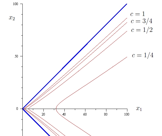
Figure 2: Plot of segments of the contours $\gamma_{0.2}(c)$ for $4c\in\{1,2,3,4\}$. The $c=1/4$ contour cuts the $x_{1}$-axis at $(1/4)^{-1/0.4}=32$.

Given ${\bf x}\in\Gamma_{\nu}(s)$ we have from (5.3) that

$$\|{\bf x}\|^{-2\nu}\leq h_{\nu}({\bf x})\leq s.$$ (5.5)

We work with a truncated version of $h_{\nu}$, namely $\tilde{h}_{\nu}:\mathbb{R}^{2}\to[0,1]$, defined for ${\bf x}\in\mathbb{R}^{2}$ by

$$\tilde{h}_{\nu}({\bf x}):=\begin{cases}\min\{h_{\nu}({\bf x}),1\}&\leavevmode\nobreak\ \leavevmode\nobreak\ \textrm{for}\leavevmode\nobreak\ \leavevmode\nobreak\ {\bf x}\in Q;\\ 1&\leavevmode\nobreak\ \leavevmode\nobreak\ \textrm{for}\leavevmode\nobreak\ \leavevmode\nobreak\ {\bf x}\in\mathbb{R}^{2}\setminus Q.\end{cases}$$

Observe that for $s>0$

$$\inf_{{\bf x}\notin\Gamma_{\nu}(s)}\tilde{h}_{\nu}({\bf x})=\min\{1,s\}.$$ (5.6)

We will derive some basic properties of the functions $h_{\nu}$ and $\tilde{h}_{\nu}$. To this end, we will use multi-index notation for partial derivatives on $\mathbb{R}^{2}$. For $\sigma=(\sigma_{1},\sigma_{2})\in\mathbb{Z}^{+}\times\mathbb{Z}^{+}$, $D_{\sigma}$ will denote $D_{1}^{\sigma_{1}}D_{2}^{\sigma_{2}}$ where $D_{j}^{k}$ for $k\in\mathbb{N}$ is $k$-fold differentiation with respect to $x_{j}$, and $D^{0}_{j}$ is the identity operator. We also use the notation $|\sigma|:=\sigma_{1}+\sigma_{2}$ and ${\bf x}^{\sigma}:=x_{1}^{\sigma_{1}}x_{2}^{\sigma_{2}}$.

Lemma 5.1

Let $\nu\in(0,1)$ and $s\in(0,1)$. Then for ${\bf x}\in\Gamma_{\nu}(s)$ and ${\bf y}=(y_{1},y_{2})$

$$\sum_{j=1}^{2}y_{j}D_{j}h_{\nu}({\bf x})=-2\nu\|{\bf x}\|^{-1}h_{\nu}({\bf x})\left(({\bf y}\cdot\hat{\bf x})-2\nu^{-1}x_{1}x_{2}\|{\bf x}\|^{2\nu-2}h_{\nu}({\bf x})({\bf y}\cdot\hat{\bf x}_{\perp})\right).$$ (5.7)

Also there exists $C\in(0,\infty)$ such that for any ${\bf x}\in\Gamma_{\nu}(s)$ and ${\bf y}=(y_{1},y_{2})$

$$\left|\sum_{j=1}^{2}y_{j}D_{j}h_{\nu}({\bf x})\right|\leq C\|{\bf y}\|\|{\bf x}\|^{2\nu-1}h_{\nu}({\bf x}).$$ (5.8)

Moreover for any ${\bf x}\in\Gamma_{\nu}(s)$, as $\|{\bf x}\|\to\infty$

$$\sup_{\sigma:|\sigma|=2}|D_{\sigma}h_{\nu}({\bf x})|=O(\|{\bf x}\|^{4\nu-2}h_{\nu}({\bf x})).$$ (5.9)

Proof. Let $\nu,s\in(0,1)$. Directly from (5.3) we obtain

$$D_{1}h_{\nu}({\bf x}) =\frac{2(1-\nu)x_{1}(x_{1}^{2}+x_{2}^{2})^{-\nu}}{x_{1}^{2}-x_{2}^{2}}-\frac{2x_{1}(x_{1}^{2}+x_{2}^{2})^{1-\nu}}{(x_{1}^{2}-x_{2}^{2})^{2}},\leavevmode\nobreak\ \leavevmode\nobreak\ \textrm{and}\leavevmode\nobreak\ \leavevmode\nobreak\$$

$$D_{2}h_{\nu}({\bf x}) =\frac{2(1-\nu)x_{2}(x_{1}^{2}+x_{2}^{2})^{-\nu}}{x_{1}^{2}-x_{2}^{2}}+\frac{2x_{2}(x_{1}^{2}+x_{2}^{2})^{1-\nu}}{(x_{1}^{2}-x_{2}^{2})^{2}}.$$ (5.10)

Since for ${\bf x}=(r,\varphi)$ in polar coordinates, for any ${\bf y}=(y_{1},y_{2})$,

$$y_{1}=({\bf y}\cdot\hat{\bf x})\cos\varphi-({\bf y}\cdot\hat{\bf x}_{\perp})\sin\varphi,\leavevmode\nobreak\ \leavevmode\nobreak\ \textrm{and}\leavevmode\nobreak\ \leavevmode\nobreak\ y_{2}=({\bf y}\cdot\hat{\bf x})\sin\varphi+({\bf y}\cdot\hat{\bf x}_{\perp})\cos\varphi,$$

it follows from (5.2) that

$$\sum_{j=1}^{2}y_{j}D_{j}h_{\nu}({\bf x}) =-\frac{2\nu(x_{1}^{2}+x_{2}^{2})^{(1/2)-\nu}}{x_{1}^{2}-x_{2}^{2}}({\bf y}\cdot\hat{\bf x})+\frac{4x_{1}x_{2}(x_{1}^{2}+x_{2}^{2})^{(1/2)-\nu}}{(x_{1}^{2}-x_{2}^{2})^{2}}({\bf y}\cdot\hat{\bf x}_{\perp})$$

$$=-\frac{2\nu(x_{1}^{2}+x_{2}^{2})^{(1/2)-\nu}}{x_{1}^{2}-x_{2}^{2}}\left({\bf y}\cdot\hat{\bf x}-2\nu^{-1}x_{1}x_{2}\|{\bf x}\|^{2\nu-2}h_{\nu}({\bf x}){\bf y}\cdot\hat{\bf x}_{\perp}\right),$$

which yields (5.7). Now from (5.7) we have that

$$\left|\sum_{j=1}^{2}y_{j}D_{j}h_{\nu}({\bf x})\right|\leq C\|{\bf y}\|\left(\|{\bf x}\|^{-1}h_{\nu}({\bf x})+h_{\nu}({\bf x})^{2}\|{\bf x}\|^{2\nu-1}\right)$$

$$\leq C\|{\bf y}\|\|{\bf x}\|^{-1}h_{\nu}({\bf x})\left(1+h_{\nu}({\bf x})\|{\bf x}\|^{2\nu}\right),$$

which with (5.5) yields (5.8). Similarly, differentiating in (5.2) and using (5.5) we obtain (5.9). $\Box$

We next show that when (5.1) holds, $(\tilde{h}_{\nu}(Z_{t}))_{t\in\mathbb{Z}^{+}}$ is a supermartingale on $\Gamma_{\nu}(s)$ for suitably small $\nu,s>0$. This is the next result.

Lemma 5.2

Suppose that (A3) holds. Suppose that for some $\beta\in(0,1)$, $c>0$, $\delta>0$, $A_{0}>0$, and $({\mathcal{F}}_{t})_{t\in\mathbb{Z}^{+}}$-stopping time $\sigma$, (5.1) and (5.2) hold. Then there exist $\nu,s\in(0,1/2)$ such that for any $t\in\mathbb{Z}^{+}$

$${\mathbb{E}}[\tilde{h}_{\nu}(Z_{t+1})-\tilde{h}_{\nu}(Z_{t})\mid{\mathcal{F}}_{t}]\leq 0$$

on $\{Z_{t}\in\Gamma_{\nu}(s)\}\cap\{t<\sigma\}$.

Proof. We suppose throughout that $t<\sigma$. Let $\nu>0$ be such that $\nu<\min\{\delta/2,(1-\beta)/8\}<1/8$. Let $s\in(0,1/2)$, to be fixed later. Note that, by (5.5), if ${\bf x}\in\Gamma_{\nu}(s)$ we have $\|{\bf x}\|>s^{-1/(2{\varepsilon})}$ and $\tilde{h}_{\nu}({\bf x})=h_{\nu}({\bf x})$. Also note that since $\tilde{h}_{\nu}({\bf x})\in[0,1]$ for all ${\bf x}$, we have

$$\left|\left(\tilde{h}_{\nu}({\bf x}+{\bf y})-\tilde{h}_{\nu}({\bf x})\right)-{\bf 1}_{\{\|{\bf y}\|<\|{\bf x}\|^{1-3\nu}\}}\left(\tilde{h}_{\nu}({\bf x}+{\bf y})-\tilde{h}_{\nu}({\bf x})\right)\right|\leq{\bf 1}_{\{\|{\bf y}\|\geq\|{\bf x}\|^{1-3\nu}\}},$$ (5.11)

for any ${\bf x},{\bf y}\in\mathbb{R}^{2}$. We have from (5.4) that there exists $C_{1}=C_{1}(s,\nu)\in(0,\infty)$ such that for all ${\bf x}\in\Gamma_{\nu}(s)$ with $\|{\bf x}\|>C_{1}$, for any ${\bf y}$ with $\|{\bf y}\|<\|{\bf x}\|^{1-3\nu}$, ${\bf x}+{\bf y}\in\Gamma_{\nu}(2s)\subset\Gamma_{\nu}(1)$. Thus Taylor’s theorem with Lagrange form for the remainder implies that for ${\bf x}\in\Gamma_{\nu}(s)$ with $\|{\bf x}\|>C_{1}$,

$${\bf 1}_{\{\|{\bf y}\|<\|{\bf x}\|^{1-3\nu}\}}\left(\tilde{h}_{\nu}({\bf x}+{\bf y})-\tilde{h}_{\nu}({\bf x})\right)={\bf 1}_{\{\|{\bf y}\|<\|{\bf x}\|^{1-3\nu}\}}\left(h_{\nu}({\bf x}+{\bf y})-h_{\nu}({\bf x})\right)$$

$$={\bf 1}_{\{\|{\bf y}\|<\|{\bf x}\|^{1-3\nu}\}}\sum_{j=1}^{2}y_{j}(D_{j}h_{\nu})({\bf x})+\frac{1}{2}{\bf 1}_{\{\|{\bf y}\|<\|{\bf x}\|^{1-3\nu}\}}\sum_{\sigma:|\sigma|=2}{\bf y}^{\sigma}(D_{\sigma}h_{\nu})({\bf x}+\eta{\bf y}),$$ (5.12)

for some $\eta=\eta({\bf y})\in(0,1)$. Taking ${\bf x}=Z_{t}$ and ${\bf y}=Z_{t+1}-Z_{t}$ and combining (5.11) and (5.12) we have that on $\{Z_{t}\in\Gamma_{\nu}(s),\|Z_{t}\|\geq C_{1}\}$,

$${\mathbb{E}}[\tilde{h}_{\nu}(Z_{t+1})-\tilde{h}_{\nu}(Z_{t})\mid{\mathcal{F}}_{t}]={\mathbb{E}}\left[{\bf 1}_{\{\|{\bf y}\|<\|{\bf x}\|^{1-3\nu}\}}\sum_{j=1}^{2}y_{j}(D_{j}h_{\nu})({\bf x})\mid{\mathcal{F}}_{t}\right]$$

$$+\frac{1}{2}{\mathbb{E}}\left[{\bf 1}_{\{\|{\bf y}\|<\|{\bf x}\|^{1-3\nu}\}}\sum_{\sigma:|\sigma|=2}{\bf y}^{\sigma}(D_{\sigma}h_{\nu})({\bf x}+\eta{\bf y})\mid{\mathcal{F}}_{t}\right]+K{\mathbb{P}}[\|{\bf y}\|\geq\|{\bf x}\|^{1-3\nu}\mid{\mathcal{F}}_{t}],$$ (5.13)

where $|K|\leq 1$.

We now deal with each of the terms on the right-hand side of (5.13) in turn. For the final term on the right-hand side of (5.13), the conditional form of Markov’s inequality and (A3) give, for ${\bf x}=Z_{t}$ and ${\bf y}=Z_{t+1}-Z_{t}$,

$${\mathbb{P}}[\|{\bf y}\|\geq\|{\bf x}\|^{1-3\nu}\mid{\mathcal{F}}_{t}]\leq\|{\bf x}\|^{6\nu-2}{\mathbb{E}}[\|Z_{t+1}-Z_{t}\|^{2}\mid{\mathcal{F}}_{t}]\leq B_{0}\|{\bf x}\|^{6\nu-2}.$$ (5.14)

The first term on the right-hand side of (5.13) may be written as

$${\mathbb{E}}\left[\sum_{j=1}^{2}y_{j}(D_{j}h_{\nu})({\bf x})\mid{\mathcal{F}}_{t}\right]-{\mathbb{E}}\left[{\bf 1}_{\{\|{\bf y}\|\geq\|{\bf x}\|^{1-3\nu}\}}\sum_{j=1}^{2}y_{j}(D_{j}h_{\nu})({\bf x})\mid{\mathcal{F}}_{t}\right],$$

where by (5.8) we have

$$\left|{\mathbb{E}}\left[{\bf 1}_{\{\|{\bf y}\|\geq\|{\bf x}\|^{1-3\nu}\}}\sum_{j=1}^{2}y_{j}(D_{j}h_{\nu})({\bf x})\mid{\mathcal{F}}_{t}\right]\right|\leq C\|{\bf x}\|^{2\nu-1}h_{\nu}({\bf x}){\mathbb{E}}\left[{\bf 1}_{\{\|{\bf y}\|\geq\|{\bf x}\|^{1-3\nu}\}}\|{\bf y}\|\mid{\mathcal{F}}_{t}\right].$$

By Cauchy–Schwarz, this last expression is bounded by

$$C\|{\bf x}\|^{2\nu-1}h_{\nu}({\bf x})\left({\mathbb{P}}[\|{\bf y}\|\geq\|{\bf x}\|^{1-3\nu}\mid{\mathcal{F}}_{t}]\right)^{1/2}({\mathbb{E}}[\|{\bf y}\|^{2}\mid{\mathcal{F}}_{t}])^{1/2}=O(\|{\bf x}\|^{5\nu-2}h_{\nu}({\bf x})),$$

by (5.14) and (A3). For the second term on the right-hand side of (5.13), we have from (5.9) that

$$\left|{\mathbb{E}}\left[{\bf 1}_{\{\|{\bf y}\|<\|{\bf x}\|^{1-3\nu}\}}\sum_{\sigma:|\sigma|=2}{\bf y}^{\sigma}(D_{\sigma}h_{\nu})({\bf x}+\eta{\bf y})\mid{\mathcal{F}}_{t}\right]\right|$$

$$\leq C\|{\bf x}+\eta{\bf y}\|^{4\nu-2}h_{\nu}({\bf x}+\eta{\bf y}){\bf 1}_{\{\|{\bf y}\|<\|{\bf x}\|^{1-3\nu}\}}=O(\|{\bf x}\|^{4\nu-2}h_{\nu}({\bf x})),$$

for ${\bf x}\in\Gamma_{\nu}(s)$ with $\|{\bf x}\|>C_{1}$. Combining these calculations we obtain from (5.13) that

$${\mathbb{E}}[\tilde{h}_{\nu}(Z_{t+1})-\tilde{h}_{\nu}(Z_{t})\mid{\mathcal{F}}_{t}]={\mathbb{E}}\left[\sum_{j=1}^{2}y_{j}(D_{j}h_{\nu})({\bf x})\mid{\mathcal{F}}_{t}\right]+O(\|{\bf x}\|^{6\nu-2}),$$ (5.15)

on $\{Z_{t}={\bf x}\}$ for ${\bf x}\in\Gamma_{\nu}(s)$ with $\|{\bf x}\|>C_{1}$, and where ${\bf y}=Z_{t+1}-Z_{t}$.

Now from (5.1) and (5.2) we have that for $\|{\bf x}\|>A_{0}$,

$${\mathbb{E}}[{\bf y}\cdot\hat{\bf x}\mid{\mathcal{F}}_{t}]\geq c\|{\bf x}\|^{-\beta},\leavevmode\nobreak\ \leavevmode\nobreak\ \leavevmode\nobreak\ |{\mathbb{E}}[{\bf y}\cdot\hat{\bf x}_{\perp}\mid{\mathcal{F}}_{t}]|=O(\|{\bf x}\|^{-\beta-\delta}).$$

Hence taking expectations in (5.7), on $\{Z_{t}={\bf x}\}$ for ${\bf x}\in\Gamma_{\nu}(s)$ with $\|{\bf x}\|$ large enough,

$${\mathbb{E}}\left[\sum_{j=1}^{2}y_{j}(D_{j}h_{\nu})({\bf x})\mid{\mathcal{F}}_{t}\right]\leq-2\nu\|{\bf x}\|^{-1}h_{\nu}({\bf x})\left[c\|{\bf x}\|^{-\beta}+O(\|{\bf x}\|^{2\nu}\|{\bf x}\|^{-\beta-\delta})\right]$$

$$\leq-2\nu\|{\bf x}\|^{-1}h_{\nu}({\bf x})\|{\bf x}\|^{-\beta}(c+o(1)),$$ (5.16)

since $\nu<\delta/2$. Noting that, by (5.5), for ${\bf x}\in\Gamma_{\nu}(s)$ we can replace the $O(\|{\bf x}\|^{6\nu-2})$ term in (5.15) by $O(\|{\bf x}\|^{8\nu-2}h_{\nu}({\bf x}))$, we obtain from (5.15) and (5.2)

$${\mathbb{E}}[\tilde{h}_{\nu}(Z_{t+1})-\tilde{h}_{\nu}(Z_{t})\mid{\mathcal{F}}_{t}]\leq-2\nu\|{\bf x}\|^{-1}h_{\nu}({\bf x})\|{\bf x}\|^{-\beta}(c+o(1)+O(\|{\bf x}\|^{\beta+8\nu-1})),$$

which is negative for all $\|{\bf x}\|$ large enough, since $\nu<(\beta-1)/8$. Also, for ${\bf x}\in\Gamma_{\nu}(s)$ we have from (5.5) that $\|{\bf x}\|\geq s^{-1/(2\nu)}$. So taking $s$ small enough, the result follows. $\Box$

Proof of Theorem 5.2. It suffices to consider wedges with principal axis in direction ${\bf e}_{1}$. First we prove the theorem for the quadrant case, $\alpha=\pi/4$. In this case, Lemma 5.2 shows that $\tilde{h}_{\nu}(Z_{t\wedge\sigma})$ is a supermartingale in $\Gamma_{\nu}(s)$ for $\nu,s$ small enough. Choose $\nu,s\in(0,1/2)$ as in Lemma 5.2, take some $K>1$ (to be fixed later) and write $\Gamma:=\Gamma_{\nu}(s)$, $\Gamma^{\prime}:=\Gamma_{\nu}(s/K)\subset\Gamma$ for this choice of parameters. Then by (5.6) and the definition of $\Gamma^{\prime}$,

$$\inf_{{\bf x}\in Q\setminus\Gamma}\tilde{h}_{\nu}({\bf x})\geq s,\leavevmode\nobreak\ \leavevmode\nobreak\ \leavevmode\nobreak\ {\rm and}\leavevmode\nobreak\ \leavevmode\nobreak\ \leavevmode\nobreak\ \sup_{{\bf x}\in\Gamma^{\prime}}\tilde{h}_{\nu}({\bf x})\leq s/K.$$

Thus Lemma 3.1 applies with $X_{t}=Z_{t\wedge\sigma}$ and $g=\tilde{h}_{\nu}$. Thus for any ${\bf x}\in\Gamma^{\prime}$, on $\{Z_{0}={\bf x}\}$,

$${\mathbb{P}}[\min\{t\in\mathbb{Z}^{+}:Z_{t\wedge\sigma}\notin\Gamma\}=\infty\mid{\mathcal{F}}_{0}]\geq 1-\frac{s/K}{s}=1-\frac{1}{K}.$$

This in turn implies that for any ${\bf x}\in\Gamma^{\prime}$, on $\{Z_{0}={\bf x}\}$,

$${\mathbb{P}}[\min\{t\in\mathbb{Z}^{+}:Z_{t\wedge\sigma}\notin Q\}=\infty\mid{\mathcal{F}}_{0}]\geq 1-\frac{1}{K},$$ (5.17)

which we can make as close to $1$ as we like by choosing $K$ large enough. Finally, since the contours $\gamma_{\nu}(c)$ eventually leave any wedge inside $Q$, we note that given $K,\nu,s$ and $\theta\in(0,\pi/4)$ we can find $A_{1}$ large enough such that $\{{\bf x}\in\mathcal{W}_{2}({\bf e}_{1};\theta):\|{\bf x}\|>A_{1}\}\subseteq\Gamma^{\prime}$. This proves Theorem 5.2 for $\alpha=\pi/4$, and hence any $\alpha\geq\pi/4$ too.

Now we extend this argument to angles $\alpha\in(0,\pi/4)$. For such $\alpha$, let ${\bf L}_{\alpha}$ denote the linear transformation of $\mathbb{R}^{2}$ defined by

$${\bf L}_{\alpha}=\left(\begin{array}[]{ll}\cos\alpha&0\\ 0&\sin\alpha\end{array}\right).$$

Then ${\bf L}_{\alpha}\mathcal{W}_{2}({\bf e}_{1};\pi/4)=\mathcal{W}_{2}({\bf e}_{1};\alpha)$.

So consider the random walk $Z_{t}$ in wedge $\mathcal{W}_{2}({\bf e}_{1};\alpha)$. Given that condition (5.1) holds in $\mathcal{W}_{2}({\bf e}_{1};\alpha)$, the same condition also holds for the walk ${\bf L}_{\alpha}^{-1}(Z_{t})$ on $\mathcal{W}_{2}({\bf e}_{1};\pi/4)$. Hence the argument for (5.17) implies that for small enough $\nu,s$ and for any ${\bf x}\in{\bf L}_{\alpha}\Gamma_{\nu}(s/K)$, on $\{Z_{0}={\bf x}\}$,

$${\mathbb{P}}[\min\{t\in\mathbb{Z}^{+}:Z_{t\wedge\sigma}\notin\mathcal{W}_{2}({\bf e}_{1};\alpha)\}=\infty\mid{\mathcal{F}}_{0}]\geq 1-\frac{1}{K},$$

and we argue as previously. This completes the proof of the theorem. $\Box$

5.3 Proof of Theorem 5.1

Proof of Theorem 5.1. The case $d=2$ of Theorem 5.1 is immediate from Theorem 5.2 on taking $Z_{t}=\xi_{t}$ and $\sigma=\infty$. So suppose $d\in\{3,4,\ldots\}$. It suffices to work with cones with principal axis in the ${\bf e}_{1}$ direction and with angle $\alpha>0$ small (but fixed). Write $C=\mathcal{W}_{d}({\bf e}_{1};\alpha)$, $d>2$. We want to show that $\Xi$ remains in $C$ with probability close to $1$ if it starts far enough ‘inside’ the cone. Let $\pi_{1},\ldots,\pi_{d-1}$ be two-dimensional projections from $\mathbb{R}^{d}$ defined by $\pi_{j}:(x_{1},\ldots,x_{d})\mapsto(x_{1},x_{j+1})$, where $j\in\{1,\ldots,d-1\}$.

For $R\subseteq\mathbb{R}^{d}$ write $\pi_{j}(R)\subseteq\mathbb{R}^{2}$ for its projection and $\Pi_{j}(R)$ for the inverse image $\pi_{j}^{-1}(\pi_{j}(R))\subseteq\mathbb{R}^{d}$, i.e., $\Pi_{j}(R):=\{(x_{1},\ldots,x_{d})\in\mathbb{R}^{d}:(x_{1},x_{j+1})\in\pi_{j}(R)\}$. For cones such as $C$, $\pi_{j}(C)$ is a wedge (a copy of $\mathcal{W}_{2}({\bf e}_{1};\alpha)$) in $\mathbb{R}^{2}$ and $\Pi_{j}(C)$ is a copy of $\pi_{j}(C)\times\mathbb{R}^{d-2}$. In particular, ${\bf x}\in\cap_{j=1}^{d-1}\Pi_{j}(C)$ implies that ${\bf x}=(x_{1},\ldots,x_{d})$ satisfies $x_{1}>0$ and $d-1$ linear inequalities each involving $x_{1}$ and one of $x_{2},\ldots,x_{d}$. Thus $\cap_{j=1}^{d-1}\Pi_{j}(C)$ is a convex rectilinear cone that contains the circular cone $\mathcal{W}_{d}({\bf e}_{1};\alpha)$. By an elementary geometrical argument, and convexity, the rectilinear cone $\cap_{j=1}^{d-1}\Pi_{j}(C)$ is contained in a circular cone $\mathcal{W}_{d}({\bf e}_{1};\alpha_{0})$ for some $\alpha<\alpha_{0}<c(d)\alpha$, where $c(d)$ is a constant depending only on the dimension $d$.

In particular, this argument shows that there exists $\alpha^{\prime}\in(0,\alpha)$ such that the $d$-dimensional circular cone $C^{\prime}=\mathcal{W}_{d}({\bf e}_{1};\alpha^{\prime})\subset C$ satisfies

$$C\supseteq\cap_{j=1}^{d-1}\Pi_{j}(C^{\prime}).$$

Thus the event

$$E:=\bigcap_{j=1}^{d-1}\{\pi_{j}(\xi_{t})\in\pi_{j}(C^{\prime})\leavevmode\nobreak\ {\rm for\leavevmode\nobreak\ all\leavevmode\nobreak\ }t\}$$

implies that $\xi_{t}\in C$ for all $t$, that is, $\tau_{\alpha}=\infty$. Thus it suffices to show that for any ${\varepsilon}>0$ we have ${\mathbb{P}}[E]\geq 1-{\varepsilon}$ provided $\xi_{0}\in C^{\prime\prime}=\mathcal{W}_{d}({\bf e}_{1};\alpha^{\prime\prime})$, with $\|\xi_{0}\|$ large enough, for some $\alpha^{\prime\prime}\in(0,\alpha^{\prime})$. Here

$${\mathbb{P}}[E]\geq 1-\sum_{j=1}^{d-1}{\mathbb{P}}[\pi_{j}(\xi_{t})\leavevmode\nobreak\ {\rm exits\leavevmode\nobreak\ from\leavevmode\nobreak\ }\pi_{j}(C^{\prime})].$$ (5.18)

Let $Z^{(j)}_{t}=\pi_{j}(\xi_{t})$ for $j\in\{1,\ldots,d-1\}$. Define the corresponding exit times

$$T_{j}=\min\{t\in\mathbb{Z}^{+}:Z^{(j)}_{t}\notin\pi_{j}(C^{\prime})\},$$

so that $\cap_{j=1}^{d-1}\{T_{j}=\infty\}$ implies $\{\tau_{\alpha}=\infty\}$. Given $\xi_{0}\in C^{\prime\prime}$ we have that $Z^{(j)}_{0}\in\pi_{j}(C^{\prime\prime})$, which is a wedge strictly contained in $\pi_{j}(C^{\prime})$. Thus Theorem 5.2 applies with $\sigma=\tau_{\alpha}$, an $({\mathcal{F}}_{t})_{t\in\mathbb{Z}^{+}}$-stopping time. Hence there exist the putative $\alpha^{\prime\prime}\in(0,\alpha^{\prime})$ and $A_{1}$ such that if $\|Z_{0}\|>A_{1}$, with probability at least $1-({\varepsilon}/d)$ the process $Z_{t\wedge\tau_{\alpha}}$ remains inside $\pi(C^{\prime})$. The same argument applies to each of the $d-1$ probabilities in (5.18), and so we have that with probability at least $1-{\varepsilon}$, $Z^{(j)}_{t\wedge\tau_{\alpha}}\in\pi_{j}(C^{\prime})$ for all $t$ and all $j$. This implies that either (i) $\tau_{\alpha}<\infty$ and $Z^{(j)}_{\tau_{\alpha}}\in\pi_{j}(C^{\prime})$ for all $j$, or (ii) $\tau_{\alpha}=\infty$. However, case (i) is impossible since by construction $Z^{(j)}_{\tau_{\alpha}}\in\pi_{j}(C^{\prime})$ for all $j$ implies that $\xi_{\tau_{\alpha}}\in C$, which is a contradiction by the definition of $\tau_{\alpha}$. Thus we conclude that ${\mathbb{P}}[\tau_{\alpha}=\infty]\geq 1-{\varepsilon}$. This completes the proof. $\Box$

5.4 Proof of Theorem 2.2

To complete the proof of Theorem 2.2, we deduce from Theorem 5.2 the existence of a limiting direction.

Proof of Theorem 2.2. Fix $\alpha>0$ (small). We show that for any ${\bf v}\in\mathbb{S}_{d}$, there is positive probability that the walk eventually remains within angle $\alpha$ of ${\bf v}$. Thus fix ${\bf v}\in\mathbb{S}_{d}$. With this $\alpha$, let $A_{1}$ and $\alpha^{\prime}\in(0,\alpha)$ be the constants in the ${\varepsilon}=1/2$ case of Theorem 5.1. Then for some $K=K(d,\alpha^{\prime})\in\mathbb{N}$ there exists a set $\{{\bf u}_{1},\ldots,{\bf u}_{K-1},{\bf u}_{K}\}\subset\mathbb{S}_{d}$ such that

$$\mathbb{R}^{d}=\bigcup_{i=1}^{K}\mathcal{W}_{d}({\bf u}_{i};\alpha^{\prime}),$$

i.e., we can write $\mathbb{R}^{d}$ as the union of $K$ cones (labelled $1,\ldots,K$) of interior half-angle ${\varepsilon}/2$. Each of the cones $\mathcal{W}_{d}({\bf u}_{i};\alpha^{\prime})$ sits inside the larger cone $\mathcal{W}_{d}({\bf u}_{i};\alpha)$. Write $B:=B_{A_{1}}$ for the ball of radius $A_{1}$. We use the notation

$$\mathcal{W}_{d}^{\prime}({\bf u};\,\cdot\,):=\mathcal{W}_{d}({\bf u};\,\cdot\,)\setminus B.$$

Consider the stochastic process

$$\Theta(t):=\max\{1\leq j\leq K:\xi_{t}\in\mathcal{W}_{d}^{\prime}({\bf u}_{j};\alpha^{\prime})\},$$

with the convention that $\max\emptyset:=0$. Thus $\Theta(t)=0$ if and only if $\xi_{t}\in B$; otherwise $\Theta(t)$ takes the label of one of the truncated cones $\mathcal{W}_{d}^{\prime}({\bf u}_{j};\alpha^{\prime})$ containing $\xi_{t}$.

Condition (A1) implies that

$$\min_{{\bf x}\in\SS\cap B}\min_{j}{\mathbb{P}}[\Xi\textrm{ hits }\mathcal{W}^{\prime}_{d}({\bf u}_{j};\alpha^{\prime})\mid\xi_{0}={\bf x}]\geq p>0.$$

It follows that a.s. there exist infinitely many times $t_{1},t_{2},\ldots$ for which $\xi_{t_{j}}\notin B$. For each $t_{j}$, we have $\Theta(t_{j})>0$. If $\Theta(t_{j})>0$, Theorem 5.1 implies that with probability at least $1/2$ (uniformly in $j$ and $\xi_{t_{j}}$) the walk remains in the larger cone $\mathcal{W}_{d}({\bf u}_{\Theta(t_{j})};\alpha)$ for all time $t\geq t_{j}$. It follows that: (i) eventually $\Xi$ remains in some cone $\mathcal{W}_{d}({\bf u}_{\Theta};\alpha)$, where $\Theta=\lim_{t\to\infty}\Theta(t)$; and (ii) ${\mathbb{P}}[\Theta=j]>0$ for all $j\in\{1,\ldots,K\}$. One consequence of (i) is that $\|\xi_{t}\|\to\infty$ a.s., i.e., the walk is transient.

In other words, (i) says that, for any $\alpha>0$, eventually the walk remains within angle $\alpha$ of some ${\bf u}_{\Theta}$, so $\xi_{t}/\|\xi_{t}\|$ has an almost sure limit. Moreover, (ii) says that with positive probability $\xi_{t}/\|\xi_{t}\|$ remains arbitrarily close to any of the ${\bf u}_{j}$, and in particular to the given vector ${\bf v}$. Thus the limit in question has distribution supported on all of $\mathbb{S}_{d}$. $\Box$

Acknowledgements

Some of this work was done when AW was at the University of Bristol, partially supported by the Heilbronn Institute for Mathematical Research.

References

- [1] S. Aspandiiarov, R. Iasnogorodski, and M. Menshikov, Passage-time moments for nonnegative stochastic processes and an application to reflected random walks in a quadrant, Ann. Probab. 24 (1996) 932–960.
- [2] R. Bañuelos and R.G. Smits, Brownian motion in cones, Probab. Theory Relat. Fields 108 (1997) 299–319.
- [3] D.L. Burkholder, Exit times of Brownian motion, harmonic majorization, and Hardy spaces, Adv. Math. 26 (1977) 182–205.
- [4] J.W. Cohen, Analysis of Random Walks, Studies in Probability, Optimization and Statistics 2, IOS Press, Amsterdam, 1992.
- [5] D. DeBlassie and R. Smits, The influence of a power law drift on the exit time of Brownian motion from a half-line, Stochastic Processes Appl. 117 (2007) 629–654.
- [6] G. Fayolle, V.A. Malyshev, and M.V. Menshikov, Topics in the Constructive Theory of Countable Markov Chains, Cambridge University Press, 1995.
- [7] A. Gut, Probability: A Graduate Course, Springer, 2005.
- [8] A. Karlsson, Linear rate of escape and convergence in direction, pp. 459–471 in: Random Walks and Geometry, V.A. Kaimanovich (Ed.), de Gruyter, 2004.
- [9] L.A. Klein Haneveld and A.O. Pittenger, Escape time for a random walk from an orthant, Stochastic Processes Appl. 35 (1990) 1–9.
- [10] J. Lamperti, Criteria for the recurrence and transience of stochastic processes I, J. Math. Anal. Appl. 1 (1960) 314–330.
- [11] J. Lamperti, Criteria for stochastic processes II: passage-time moments, J. Math. Anal. Appl. 7 (1963) 127–145.
- [12] G.F. Lawler, Estimates for differences and Harnack inequality for difference operators coming from random walks with symmetric, spatially inhomogeneous, increments, Proc. London Math. Soc. 63 (1991) 552–568.
- [13] G.F. Lawler, Intersections of Random Walks, Probability and Its Applications, Birkhäuser, Boston, 1996.
- [14] G.F. Lawler, Conformally Invariant Processes in the Plane, American Mathematical Society, 2005.
- [15] I.M. MacPhee, M.V. Menshikov, and A.R. Wade, Exit times from cones for non-homogeneuos random walk with asymtptoically zero drift, Preprint arXiv:0806.4561.
- [16] M.V. Menshikov, I.M. Asymont, and R. Iasnogorodskii, Markov processes with asymptotically zero drifts, Problems of Information Transmission 31 (1995) 248–261; translated from Problemy Peredachi Informatsii 31 (1995) 60–75 (in Russian).
- [17] M.V. Menshikov and S.Yu. Popov, Exact power estimates for countable Markov chains, Markov Processes Relat. Fields 1 (1995) 57–78.
- [18] M.V. Menshikov, M. Vachkovskaia, and A.R. Wade, Asymptotic behaviour of randomly reflecting billiards in unbounded tubular domains, J. Stat. Phys. 132 (2008) 1097–1133.
- [19] M.V. Menshikov and A.R. Wade, Random walk in random environment with asymptotically zero perturbation, J. Euro. Math. Soc. 8 (2006) 491–513.
- [20] S. Mustapha, Gaussian estimates for spatially inhomogeneous random walks on , Ann. Probab. 34 (2006) 264–283.
- [21] Z. Shi, Windings of Brownian motion and random walks in the plane, Ann. Probab. 26 (1998) 112–131.
- [22] F. Spitzer, Some theorems concerning -dimensional Brownian motion, Trans. Amer. Math. Soc. 87 (1958) 187–197.
- [23] F. Spitzer, Principles of Random Walk, 2nd edition, Springer, New York, 1976.
- [24] N.Th. Varopoulos, Potential theory in conical domains, Math. Proc. Camb. Phil. Soc. 125 (1999) 335–384.
- [25] O. Zeitouni, Random walks in random environments, J. Phys. A 39 (2006) R433–R464.